Lists in a Lighthouse

(1)

University of South Carolina

Scholar Commons

Theses and Dissertations

12-14-2015

Confluence of Density Currents Over an Erodible

Bed

Hassan Ismail

University of South Carolina - Columbia

Follow this and additional works at:https://scholarcommons.sc.edu/etd Part of theCivil Engineering Commons

This Open Access Thesis is brought to you by Scholar Commons. It has been accepted for inclusion in Theses and Dissertations by an authorized administrator of Scholar Commons. For more information, please [email protected].

Recommended Citation

Ismail, H.(2015).Confluence of Density Currents Over an Erodible Bed.(Master's thesis). Retrieved from

(2)

Confluence of Density Currents Over an Erodible Bed

by

Hassan Ismail

Bachelor of Science

University of South Carolina 2011

Submitted in Partial Fulfillment of the Requirements

for the Degree of Master of Science in

Civil Engineering

College of Engineering and Computing

University of South Carolina

2015

Accepted by:

Jasim Imran, Director of Thesis

Enrica Viparelli, Reader

M. Hanif Chaudhry, Reader

(3)

c

(4)

Dedication

(5)

Abstract

Results from laboratory experiments on conservative density current confluence

are reported. Hydraulic characteristics and morphodynamic consequences of the

con-fluence of two continuous release density currents in a horizontal, 45◦ asymmetrical

junction are examined and compared to those of terrestrial river junctions. It was

observed that density current confluence is markedly different than those in river

junctions primarily due to the ease of the dense fluid to convect into the ambient

fluid in the junction zone. Upward convection in the junction resulted in low

horizon-tal velocity and shear stresses on the bed of the junction zone, followed by re-plunging

to the layer of neutral buoyancy downstream of the junction where acceleration

oc-curs. In the downstream reach was a distinctive erosional pattern similar to central

scouring seen in river junctions but starting at the downstream junction point rather

than at the upstream junction point. It was found that terrestrial river models match

well with the density current case in terms of maximum velocity downstream of the

junction, backwater effect, avalanche face protrusion into the downstream reach, and

maximum scour orientation. Poor matching was found in terms of separation zone

dimensions and shape, streamline deviation angle on the junction line, and maximum

(6)

List of Figures

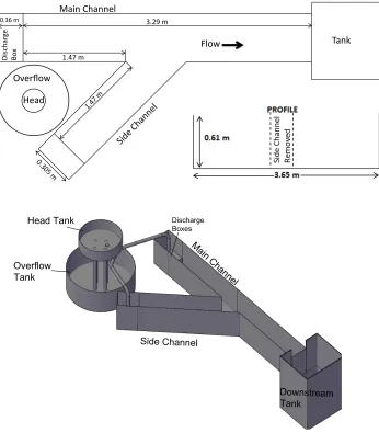
Figure 3.1 Physical model dimensions in plan view, profile view, and rendering. 17

Figure 3.2 Comparison of main channel and side channel primary velocity

at the channel centerlines. . . 18

Figure 3.3 Initial head confluence of the density currents in time as seen

from the main channel. . . 18

Figure 3.4 Primary velocity profiles along the main channel centerline. Solid vertical lines indicate the points of measurement, and dashed vertical lines indicate the location at which the side

channel connects. . . 18

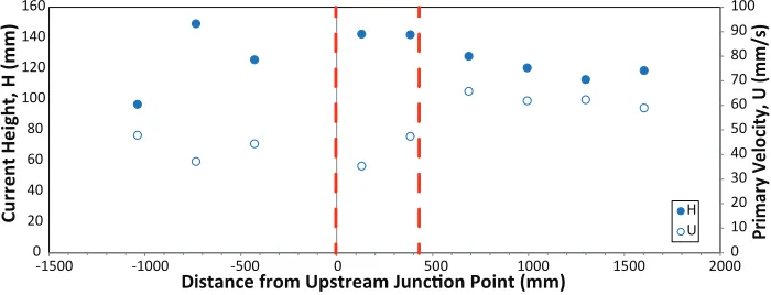
Figure 3.5 Layer averaged current height and velocity based on 1D profiles. . 19

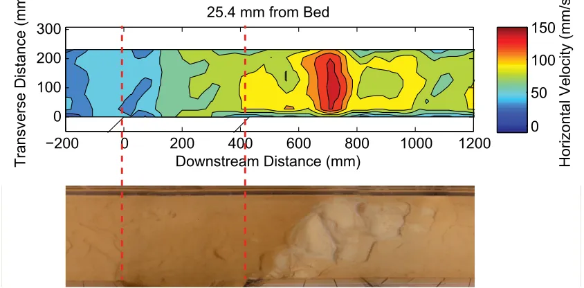
Figure 3.6 Horizontal isovelocity map near the junction zone at 114.3 mm, 88.9 mm, 63.5 mm, 38.1 mm, and 25.4 mm from the bed. The

origin of the plot is the upstream junction point. . . 20

Figure 3.7 Horizontal velocity vectors with streamlines near the junction zone at 114.3 mm, 88.9 mm, 63.5 mm, 38.1 mm, and 25.4 mm

from the bed. The origin of the plot is the upstream junction point. 21

Figure 3.8 Evolution of the bed of main channel after 540 s, 1028 s, 3630 s, 4140 s, 5618 s, and 9329 s total run time. Flow is from left to right, and the vertical dash lines indicate the locations of the

junction points. . . 22

Figure 3.9 Qualitatively observed erosional pattern downstream of the junction. 22

Figure 3.10 Near-bed velocity isoline plot with associated scouring down-stream of the junction. The dashed vertical lines indicate the

(8)

Figure 4.1 Typical characteristics of river channel confluences (left panel) and observed characteristics of density current confluences (right

panel). . . 31

Figure 4.2 Zoomed streamlines near flow separation zone. The dash line indicates the extent of the flow separation zone, and the coordi-nates X and Y indicate the downstream and lateral coordicoordi-nates,

respectively, of the points of interest. . . 32

Figure 4.3 Variation of streamline deviation angle from the upstream to

downstream junction points. . . 33

Figure 4.4 Variation of streamline deviation angle with depth. Included is

the fit curve to the density current case. . . 33

Figure 4.5 Visual method for measuring current height downstream and

upstream of the junction. . . 34

Figure 4.6 Location and extent of avalanche face protrusion into the

down-stream reach. . . 34

(9)

Chapter 1 Introduction

Density currents are flows driven by the density difference between a current and

ambient fluid (Benjamin 1968). This density difference may be caused by a

conser-vative substance such as dissolved salt, or by a non-conserconser-vative substance such as

suspended sediment. In particular, turbidity currents are sediment-laden underflows

that may travel for very long distances on the ocean floor. They can create

self-forming canyons and channels passing over the continental slope and into the abyssal

plane (Peakall, McCaffrey, and Kneller 2000). After the slope break at the toe of

the continental slope, turbidity currents can deposit their suspended sediments in

submarine fans.

Natural turbidity currents are episodic events that, depending on the triggering

mechanism and conditions, can be either sustained, quasi-steady flows or surge-type

events (Hay 1987). The episodic nature of turbidity currents has left only a few notable

instances of direct field observation of turbidity current flows (e.g., Prior et al. 1987;

Normark 1989; Khripounoff et al. 2003; Paull et al. 2002; Xu, Noble, and Rosenfeld

2004; Vangriesheim, Khripounoff, and Crassous 2009).

Although a great deal of attention has been placed on the study of submarine

channel systems, previous studies have focused heavily on the hydraulics and

mor-phodynamics of individual channels and sinuous submarine channels (e.g., Keeulegan

1949; Simpson and Britter 1979; Parker, Fukushima, and Pantin 1986; Parker et al.

1987; Garcia and Parker 1993; Kneller, Bennett, and McCaffrey 1999; Peakall,

(10)

Imran, and Pirmez 2008; Islam and Imran 2008; Sequeiros et al. 2010; Huang, Imran,

and Pirmez 2012; Ezz, Cantelli, and Imran 2013; Janocko et al. 2013; Tokyay and

Garcia 2013). Although submarine channel networks and confluences are well

doc-umented through field observation (Canals, Urgeles, and Calafat 2000; Dalla Valle

and Gamberi 2011; Greene, Maher, and Paull 2002; Hesse 1989; L’Heureux, Hansen,

and Longva 2009; Mitchell 2004; Paquet et al. 2010; Straub et al. 2011, e.g.,), little

attention has been placed on understanding the characteristics and physical processes

of these settings.

Hesse (1989) and Klaucke, Hesse, and Ryan (1998) acquired imagery data of the

Labrador sea floor including an extensive network of converging drainage channels.

Based on seismic and sonar data, distinct differences between submarine and

sub-aerial drainage systems were identified. Mitchell (2004) and Vachtman, Mitchell, and

Gawthorpe (2013) described erosion rates and submarine canyon hydrology on the

Atlantic continental slope and recommended a simple relationship to describe erosion

rates as a function of channel gradient and contributing area. To do so, the authors

employed principles of terrestrial hydrology to the submarine environment. An

impor-tant assumption in developing their model is that long-term erosion rates of branches

of fluvial (and thus extended to submarine) channels must be identical. Straub et

al. (2007) used high resolution data from the Monterey, CA and Brunei Darussalam

continental slopes to assess submarine channel profiles and drainage area statistics.

Although substantial differences in physical processes exist, the data yielded

subma-rine scaling exponents within the range of terrestrial observations.

Gamboa, Alves, and Cartwright (2012) provides the most detailed survey of

sub-marine confluences on confined slopes (i.e., subsub-marine canyon confluences). Based

on the interpretation and analysis of 3D seismic data, these researchers proposed a

classification scheme based on the geometry of the confluence. The classification

(11)

which case the downstream reach is in line with one of the contributing channels, or

symmetrical, in which case the downstream reach approximately bisects the junction

angle between the contributing channels. Confluence densities and width ratios in the

study area of Gamboa, Alves, and Cartwright (2012) also indicate similarities to those

found in fluvial river systems furthering the notion by Mitchell (2004) and Straub

et al. (2007) that submarine channel confluences, from the drainage and hydrological

perspective, are similar to those found in terrestrial river systems.

Despite the similarities noted in geometry and erosion rates, hydraulic differences

in the confluences of submarine channels inevitably exists due to the nature of density

currents. The most significant difference hydraulically is that the density contrast

be-tween turbidity currents and the ambient fluid is on the order of only a few percent,

whereas fluvial rivers experience a density difference of about 800 times that of the

ambient fluid (i.e., air) (Parker, Fukushima, and Pantin 1986; Imran, Parker, and

Katopodes 1998). Some aspects of turbidity or density currents have been well

doc-umented as analogous to rivers and others have shown distinct differences. Several

researchers (e.g., Clark and Pickering 1996; Peakall, McCaffrey, and Kneller 2000;

Pirmez and Imran 2003) document the similarities in sinuosity, wavelengths, and

avulsions of submarine channels and river channels. Others document the differences

in terms of hydraulic and morphodynamic character (e.g., Parker, Fukushima, and

Pantin 1986; Wynn, Cronin, and Peakall 2007; Kolla, Posamentier, and Wood 2007;

Deptuck et al. 2007; Islam and Imran 2008; Sequeiros et al. 2010; Straub et al. 2011;

Ezz and Imran 2014). Parker et al. (1987) noted that since relative density is the

driving mechanism of turbidity currents, erosive and flow power are subject to direct

feedback from entraining and depositing bed sediment adding complexity to sediment

transport potential in submarine flows. Sequeiros et al. (2010) proposed a sediment

transport relation which is strikingly similar to that of river systems with

(12)

channels can be a result of aggradation rather than incision as is the case with river

channels. To the authors’ knowledge, no study has been reported regarding hydraulics

and sediment response in submarine channel confluences despite the fact that channel

networks are important elements of continental margin strata.

This paper presents the results and the analysis of laboratory experiments

specif-ically designed to study simultaneously active, conservative density current

conflu-ences over an erodible bed. Using the classification system of Gamboa, Alves, and

Cartwright (2012), tests were performed in a neutrally asymmetric confluence

(neu-trally indicating that both upstream reaches contribute equally to the downstream

reach). A total of 21 subsequent density currents were released to characterize the

velocity field in the junction and in the contributing channels. In particular,

one-dimensional primary (i.e., streamwise) velocity and two-one-dimensional horizontal

ve-locity in the near junction zone were measured. Further, qualitative assessment of

bed evolution was performed after each test. Well-established models for terrestrial

river confluences were then tested with the submarine data to identify similarities

and differences between subaerial and submarine confluences. This study focused on

gaining insight on the hydraulics and mechanics of density current confluences and

their morphological impacts, and on observing how the submarine velocity field and

(13)

Chapter 2 Background Information on River Confluences

The characteristics and properties of river channel confluences have been examined by

field observations (e.g., Best 1988), physical experiments (e.g., Lin and Soong 1979;

Best 1988; Gurram, Karki, and Hager 1997; Hsu, Wu, and Lee 1998; Webber and

Greated 1966; Qing-Yuan et al. 2009), and theoretical and numerical models (e.g.,

Lin and Soong 1979; Hsu, Wu, and Lee 1998; Hsu, Lee, and Chang 1998; Shabayek,

Steffler, and Hicks 2002; Kesserwani et al. 2008).

Hydraulic characteristics in terrestrial river confluences include a separation zone

downstream of the junction, streamline deviation angle from the side channel, and a

backwater effect into each contributing reach.

In the confluence of terrestrial rivers, flow separation occurs at the downstream

junction point and continues into the downstream reach; the extent of flow separation

has been studied by Best and Reid (1984) and Gurram, Karki, and Hager (1997) who

both focused on maximum separation zone dimensions, and Qing-Yuan et al. (2009)

who studied the variation in separation zone geometry with depth.

Best and Reid (1984) quantified the geometry and extent of the flow separation

zone downstream of an experimental, equal-width junction. They varied both relative

discharge and junction angle and tracked the extent of the separation zone visually

using an overhead camera. The authors found that the length and width of the

flow separation zone increase with both relative tributary contribution and junction

angle. Best and Reid (1984) fit logarithmic trend lines to their data set for maximum

(14)

bs

b3

= 0.264 + 0.117 ln(Qs Qm

) (2.1)

Ls

b3

= 1.348 + 0.538 ln(Qs Qm

) (2.2)

where bs and Ls are the width and length of the separation zone, respectively, b3

is the width of the downstream reach,Qs is the discharge from the side channel, and

Qm is the discharge from the side channel. Gurram, Karki, and Hager (1997) also

developed an analytical solution for separation zone geometry in subcritical

open-channel flows as:

bs

b3 = 1

2(Fd/s− 2 3)

2_{+ 0} .45Q

1 2 r(

θ

90◦) (2.3)

Ls

b3

= 3.8 sin3θ(1− 1

2Fd/s)Q

1 2

r (2.4)

where Fd/s is the downstream Froude number, Qr is the discharge ratio, and θ is

the junction angle.

Qing-Yuan et al. (2009) furthered the investigation into separation zone geometry

by describing the variation of separation zone extent with depth in a 90◦ open channel

junction. In particular, they developed a new method for defining the extent of

the separation zone called the velocity isoline method which is based on tracing

the zero-downstream-velocity contour to define the separation zone boundary. The

careful comparison of the new isoline method with the classical streamline method

to determine the extent of the separation zone revealed that the isoline method is

simpler to implement if velocity data is available. The main results of the Qing-Yuan

et al. (2009) work are, 1) the separation zone at open channel junctions increases

both in width and in length away from the bed, and 2) the separation zone becomes

(15)

Due to flow separation in the downstream reach of river confluences, effective flow

area decreases opposite to the separation zone creating a high velocity region alongside

the separation. Best and Reid (1984) defined a velocity index for the maximum near

bed velocity as Ux =Umax/U1 where Ux is the velocity index, Umax is the maximum

observed velocity in the downstream reach at the separation zone section, and U1 is

the velocity in the main upstream reach. A line was fit to the data as:

Ux= 4.52 + 2.36

b3−bs

b3

(2.5)

Early models of river confluences (e.g., Lin and Soong 1979), termed linear models,

assumed equal upstream water depths in each contributing branch. Later models of

Hsu, Lee, and Chang (1998) and Gurram, Karki, and Hager (1997), are nonlinear

models based on momentum balance in the junction.

Hsu, Lee, and Chang (1998) proposed an analytical approach for solving the

up-stream depth ratio of subcritical open channel junction flows for equal width,

hori-zontal channels and they found that the upstream depth ratio is directly correlated

to the Froude number in the downstream reach, Fd/s, and to junction angle. The

re-searchers also examined trends of streamline deviation angle across the junction line

as a function of discharge ratio and junction angle. The deviation angle is defined as

the angle of the streamlines entering the junction from the side channel. The

devia-tion angle is measured relative to the juncdevia-tion line, and the side channel streamlines

are skewed from the junction angle due to forcing from the main channel inflow.

The pioneering work of Best (1988), which included both laboratory experiments

and field observation, utilized knowledge of junction hydraulics to identify three

dis-tinct morphological elements common among open channel junctions: 1) avalanche

faces at the upstream edges of the junction zone where the two contributing channels

combine, 2) a deep central scour beginning at the upstream junction point and

(16)

of the separation zone. The dominant factors effecting the geometry of these three

elements are relative discharge and junction angle. Best (1988) concluded that

in-creasing either of these factors, i.e., the relative discharge and/or the junction angle,

results in a more pronounced segregation of sediment and flow contributions causing

1) the retreat of the main channel avalanche face, 2) rotation of the central scour

about the upstream junction point, and 3) increase in the extent of the separation

zone bar. Gamboa, Alves, and Cartwright (2012) identified morphological elements of

submarine junctions that are similar to those defined by Best (1988), i.e., the presence

of plunging faces in the contributing channels and a well defined scour int he

junc-tion zone. These observajunc-tions suggest that by using the well-established knowledge

on fluvial channel confluences, analogies between the subaerial and the submarine

settings can be established.

By relating protrusion into the junction with relative discharge and junction angle,

Best (1988) fit a line to his data for the case of equal contribution from each channel

as:

= 1.9525−0.0186θ (2.6)

whereis the normalized distance from the upstream junction point to the farthest

point of the avalanche face into the junction and is normalized by the downstream

channel width as=a/b3whereais the dimensional maximum extent of the avalanche

face into the junction from the upstream junction point.

Best (1988) also developed logarithmic trend lines for the maximum depth of

scouring past the avalanche face starting at the upstream junction point. The depth

of scouring was normalized by the upstream reaches’ water depth and takes the form:

ds =−4.944 + 1.830 lnθ (2.7)

(17)

dimensional scour depth and Yavg is the average water depth of the main and side

channels at the junction entrance.

Best (1988) has described the orientation of the line of maximum scour as

approx-imately bisecting the junction angle which was computed from the curve for equal

upstream discharge taking the form:

β = 6.98 + 0.297θ (2.8)

where β is the angle of the maximum scour line relative to the main channel

(18)

Chapter 3 Laboratory Experiments

3.1 Experimental Setup and Procedure

The laboratory experiments were conducted in an asymmetric y-shaped flume in the

Hydraulics Laboratory at the University of South Carolina (Figure 3.1). Experimental

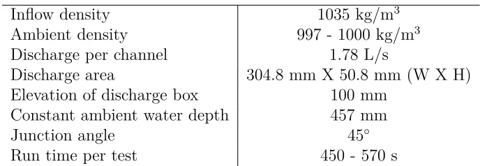
conditions are summarized in Table 3.1.

Experimental Conditions

The rigid sub-bed of the flume was constructed with painted wood. The walls were

painted wood on one side of the flume and transparent acrylic glass on the other side

for flow visualization and tracking of the density current’s propagation.

The near-junction zones, to a distance of 0.91 m in the upstream direction and

the entire length of the downstream reach, was covered to a depth of 40 mm with

sand-sized plastic particles with a specific gravity of 1.5 and D50 of 0.2 mm. The

extreme upstream reaches of each inflow channel was a painted wood board to allow

the current to develop fully before reaching the erodible bed material. The board was

also 40 mm deep to avoid any bed discordance.

A premixed salt water solution was stored in a continuously stirred overflow tank

from which it was lifted to a constant-elevation head tank. The head tank split in a

manifold to feed each upstream reach. Each limb of the manifold was equipped with

differential piezometers and valves to monitor and ensure constant inflow throughout

(19)

box and grate to ensure the inflow was quiescent and the density current could form

in a relatively short downstream distance. The discharge boxes were elevated to 100

mm above the flume bed to allow the inflow mixture to plunge to produce a coherent

density current. The flume’s downstream reach terminated in a large tank where the

density current was allowed to plunge below the flume’s bed elevation. The ambient

water level was maintained with an overflow drain pipe in the downstream tank.

Test Procedure

In preparation for each test, 1.28 m3_{of a salt water mixture was prepared to a density}

of 1035 kg/m3. To this end, a bench test was performed to determine the precise mass

of salt required for each incremental change in fluid density. Using the results of the

bench test, a formula was developed based on the initial density of the fluid and

target density as:

msalt

∀ = 1.366×(ρtarget−ρinitial) (3.1)

where msalt is the required mass of salt in kg,∀ is the volume of the container in

m3_,_ρ

target is the desired final density of the solution in kg/m3, and ρinitial is the initial

density of the water in kg/m3_{. Since, depending on the run time off each test, the}

entire pre-mixed volume was not fully used, before the subsequent test the mixing

tank was refilled with fresh water, mixed, and the initial density was measured in

preparation for the new mixture. This procedure resulted in reliably constant inflow

density for all tests.

Before the test runs begin, the flume was filled with fresh water, and a continuously

operating submersible pump was used to elevate the salt water mixture to a head tank.

Once the head tank begins to overflow back to the storage tank for a suitable amount

of time, testing can begin. For the duration of the test, a calibrated discharge pump

(20)

of the flume. In tandem, a constant, low-velocity inflow of fresh water was added

to the top of the downstream discharge tank to reduce upward convection of dense

water in the downstream tank and to prevent reflection. Each test was initiated by

simultaneously opening valves releasing the salt water mixture to each flume. Using

the differential piezometers, all tests showed a constant inflow of 1.78 L/s (±2%) to

each channel. The discharge started in the momentum-reducing boxes, passed the

flow-straightening grates, and formed two developed density currents. The currents’

heads propagated downstream, collided at the junction, and continued downstream.

Once the head of the combined current exited the domain and the current height

stabilized, measurement procedures began.

Once the pre-mixed volume of salt water was nearly depleted, the test was halted

by closing the inflow valves to each discharge box. The current tail was then allowed

to move downstream where the discharge pump and drain were still active until the

current exited the domain completely. The flume was then drained to approximately

one-third of the initial depth, and photographs of the bed were taken. To avoid any

bed disturbance, the flume was never completely drained below this point between

tests; rather, the flume was slowly refilled with fresh water and drained repeatedly

until the water density was measured to be 1000 kg/m3_{, as desired, for subsequent}

testing.

Measurement Techniques

Measurements were taken to capture the current depth in space, 1D velocity profiles,

2D horizontal velocity, and bed evolution after each test. A high-definition camcorder

was mounted along the flume’s main channel to capture the current development in

space and time. In preliminary testing, these cameras were also used to ensure the side

and main channels were behaving similarly in terms of density current development

(21)

45◦ pointing downward into the current for 1D primary velocity measurement as a

function of depth. These probes were placed at the centerline of the main and side

channels and downstream reach. UVPs were also used in a grid pattern to obtain

2D horizontal velocity at 114.3, 88.9, 63.5, 38.1, and 25.4 mm from the bed. The

near-bed 2D velocity was used to correlate to observations on bed development. A

still overhead camera was used to photograph the bed of the main channel after each

run. For better quality of the photos, several photos were taken at a short distance

from the bed and merged to one image. The photos were overlapped approximately

30% on each side to avoid distortion in the final image.

3.2 Flow Field

Given equal inflow discharges to each flume, behavior of each upstream reach was

established to be equal by obtaining primary, or downstream, velocity profiles in

the channel centerlines at 1.092 m from each discharge boxes. Figure 3.2 shows

the normalized velocity profile from each channel and good agreement is observable.

The peak velocity is within 8% in each channel with similar shape and inflection

(near z/H = 1). In the figure, z is the upward coordinate from the bed, u is the

measured primary velocity, andU and H are the depth averaged velocity and current

height, respectively, by using the moment method (Parker et al. 1987). Since matching

between the side and main channel is good, henceforth measurements and discussion

will focus on the main upstream channel, junction zone, and the downstream reach.

In the laboratory tests it was observed that the current rose into the ambient

water layer in the junction as seen in Figure 3.3 taken during the initial collision of

the current fronts. After the two inflows combined, they re-plunged in the downstream

reach. This large plume subsided to a quasi-equilibrium height which is represented

in the velocity profiles of Figure 3.4 and the depth-averaged H in Figure 3.5. The

(22)

Primary Velocity

Figure 3.4 shows one-dimensional primary velocity along the main channel centerline.

The dashed vertical lines in the figure indicate the upstream and downstream

junc-tion points, and the solid vertical lines indicate the measurement point downstream

coordinate. The maximum velocity near the junction shifted away from the bed near

the downstream junction point and then returned to a more typical velocity profile

in the downstream reach.

Figure 3.5 shows the layer-averaged current thickness, H, and velocity, U based

on the profiles seen in Figure 3.4. As expected for the majority of the domain,H and

U were inversely correlated, but both increased near the downstream junction point.

This suggests that in the junction zone, there was significant upward convection of

momentum causing the maximum velocity to be further from the bed and flow area

to increase.

Horizontal Velocity

Two-dimensional horizontal velocity measurements were taken near the junction at

five different elevations above the bed. Isovelocity maps are shown in Figure 3.6; the

entire width of the main channel is not included in these measurements due to the

need for physical clearance of the velocity probes. In general, velocity in the junction

zone and downstream of the junction was higher closer to the bed as expected based

on the one-dimensional velocity profiles in Figure 3.4. At all of the five elevations near

the upstream junction point, horizontal velocity was low with acceleration through

the junction zone and in particular downstream of the junction. Some flow separation

can be noted just beyond the downstream junction point which is more evident away

from the bed.

Horizontal velocity vectors with streamlines are shown in Figure 3.7. A clear

(23)

Near the bed, the main channel contribution was restricted to the outer wall of the

downstream reach as the side channel inflow entered the junction. Conversely, the

main channel contribution was more dominant away from the bed. This implies that

the main channel flow rode atop the side channel flow in the junction before mixing in

the downstream reach where velocity was once again unidirectional. The stagnation

of flow near the upstream junction point seen in the horizontal velocity contour plots

(Figure 3.6) can also be seen in the streamlines plots (Figure 3.7) where streamlines

near the upstream junction point in the main channel terminate against the shear

plane of contributing inflows. Flow separation in the downstream reach is also evident

in termination of streamlines against the wall of the flume at elevations far from the

bed. It can be inferred that the main channel inflow rode atop the side channel inflow

and entrained ambient water, thus becoming more diffuse and weaker. Its ability to

counteract the momentum from the side channel lessened allowing for the formation

of a downstream separation zone. Near the bed, the orientation of the downstream

reach and strength of the main channel inflow forced the side channel contribution

to deviate to the downstream direction and stick to the wall of the flume.

3.3 Bed Evolution

Figure 3.8 shows the evolution of the erosional pattern observed on the bed. The

inflow condition was such that sufficient shear stress was acting on the bed to create

distinctive bedforms upstream and downstream of the junction zone, but very little

sediment transport was noted in the junction zone itself. This corroborates the notion

that horizontal momentum was converted to vertical momentum in the confluence

zone as the main channel inflow rose above the side channel inflow. Thus horizontal

shear stresses acting on the bed were reduced inhibiting transport of bed material.

The most distinctive bathymetric pattern was the scouring beginning at the

(24)

Table 3.1 Experimental conditions.

Inflow density 1035 kg/m3

Ambient density 997 - 1000 kg/m3

Discharge per channel 1.78 L/s

Discharge area 304.8 mm X 50.8 mm (W X H)

Elevation of discharge box 100 mm

Constant ambient water depth 457 mm

Junction angle 45◦

Run time per test 450 - 570 s

the flume. The avalanche face (i.e., beginning of the scoured section) was

approxi-mately in line with the side channel’s wall and developed a series of relatively deep

erosional waves from successive runs until reaching the opposite wall (Figure 3.9).

By comparing the scouring to the near-bed velocity contours (Figure 3.6), it is clear

that this zone downstream of the junction experiences the highest horizontal velocity,

thus scouring here is expected.

Figure 3.10 shows the near-bed velocity and associated scouring downstream of

the junction. From this plot it is clear that in the junction there was relatively low

horizontal velocity thus sediment transport capacity was limited. However,

down-stream of the junction, high horizontal velocity indicates high bed shear stress which

(25)

Head Tank

Main Channel

Side Channel

Overflow Tank

Discharge Boxes

Downstream Tank 1.47 m

Di

sc

ha

rg

e

Bo

x

Main Channel

Flow Tank

0.36 m _{3.29 m}

Overﬂow

Head

0.305 m

(26)

0.0 0.2 0.4 0.6 0.8 1.0 1.2

-0.5 0.0 0.5 1.0 1.5

N or m al iz ed D is ta nc e fr om B ed (z /H )

Normalized Downstream Velocity (u/U)

Main Channel Side Channel

Figure 3.2 Comparison of main channel and side channel primary velocity at the channel centerlines.

FLOW FLOW

Figure 3.3 Initial head confluence of the density currents in time as seen from the main channel. 50 mm/s 0 50 100 150 200 250

-1500 -1000 -500 0 500 1000 1500 2000

Di st an ce fr om B ed (m m )

Distance from Upstream Junction Point (mm)

(27)

0 10 20 30 40 50 60 70 80 90 100 0 20 40 60 80 100 120 140 160

-1500 -1000 -500 0 500 1000 1500 2000

Pr im ar y Ve lo cit y, U (m m /s ) Cu rr en t H ei gh t, H (m m )

Distance from Upstream Junction Point (mm)

H U

(28)

Downstream Distance (mm)

Transverse Distance (mm)

114.3 mm from Bed

−200 0 200 400 600 800 1000 1200

0 100 200 300

Horizontal Velocity (mm/s)

0 50 100 150

88.9 mm from Bed

−200 0 200 400 600 800 1000 1200

0 100 200 300

0 50 100 150

63.5 mm from Bed

−200 0 200 400 600 800 1000 1200

0 100 200 300

0 50 100 150

38.1 mm from Bed

−200 0 200 400 600 800 1000 1200

0 100 200 300

0 50 100 150

25.4 mm from Bed

−200 0 200 400 600 800 1000 1200

0 100 200 300

0 50 100 150

(29)

−200 0 200 400 600 800 1000 1200 0

100 200 300

114.3 mm from Bed

−200 0 200 400 600 800 1000 1200 0

100 200 300

88.9 mm from Bed

−200 0 200 400 600 800 1000 1200 0

100 200 300

63.5 mm from Bed

−200 0 200 400 600 800 1000 1200 0

100 200 300

38.1 mm from Bed

−200 0 200 400 600 800 1000 1200 0

100 200 300

25.4 mm from Bed

Junction Line 100 mm/s

(30)

540 s

1028 s

3630 s

4140 s

5618 s

9329 s

Figure 3.8 Evolution of the bed of main channel after 540 s, 1028 s, 3630 s, 4140 s, 5618 s, and 9329 s total run time. Flow is from left to right, and the vertical dash lines indicate the locations of the junction points.

Junction Line

(31)

25.4 mm from Bed

−200 0 200 400 600 800 1000 1200

0 100 200 300

0 50 100 150

(32)

Chapter 4 Comparison to River Confluences

4.1 Comparison to River Hydraulics

With the previously discussed observations and measurements, comparisons can be

directly made to well-established observations of subaerial river confluences. This

comparison will focus on comparing hydraulic response to the confluence as described

by Best and Reid (1984), Gurram, Karki, and Hager (1997), Hsu, Lee, and Chang

(1998), and Qing-Yuan et al. (2009). Morphological characteristics of river confluences

are extracted from the work of Best (1988). Hydraulic characteristics to be assessed

include 1) flow separation downstream of the junction; 2) maximum velocity due to

the effective flow contraction adjacent to the separation zone; 3) deviation angle of

streamlines entering from the side channel; and 4) backwater effect of the junction into

the upstream reaches. Morphological features that are assessed include 1) avalanche

faces at the edge of scouring in the junction zone; 2) maximum scouring depth; and 3)

maximum scouring orientation. Figure 4.1 shows these characteristics as expected in

river confluences with a summary of the characteristics found in the density current

case.

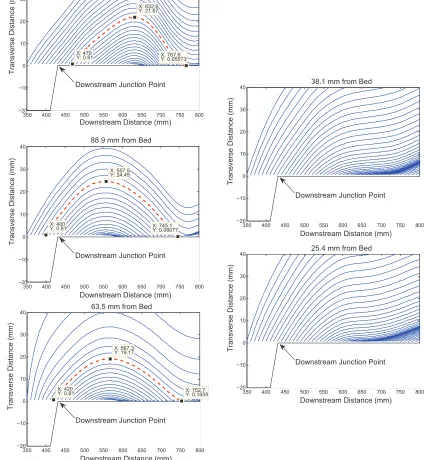
Separation Zone

The zero-velocity contour at most elevations are hardly visible in the contour plots

of Figure 3.6. Furthermore a closer view and finer contouring revealed only minimal

(33)

Figure 4.2 shows closer views of the streamlines presented in Figure 3.7. Very distinct

separation can be seen for the upper three elevations at which horizontal velocities

were measured. It is also clear from this figure that near the bed, flow does not

sep-arate from the downstream wall. To define coordinates of the streamline delineating

the separation zone, the farthest streamline downstream to reattach to the wall was

traced upstream to its point of origin. This data is summarized in Table 4.1 in which

x1 and x2 are the downstream coordinates of the streamline beginning and end,

re-spectively, and Ls and bs are the separation zone length and width, respectively. By

comparing the ability to define the separation zone by either the streamline or isoline

method, it was found that the streamline method performs better than the isoline

method when velocity data is available.

By applying Equations 2.1-2.4 to the current work, the predicted maximum width

and length of the separation zone are presented in Table 4.1. In both models,

sepa-ration zone width is over predicted and length is under predicted. The model of Best

and Reid (1984) matched modestly better than the analytical solution of Gurram,

Karki, and Hager (1997) indicating that although separation can occur in the case

of density currents, application of an analytical solution solved for subaerial flows is

inappropriate for application for submarine flows.

To apply the Gurram, Karki, and Hager (1997) solution, Fd/s was computed as:

Fd/s=

Qt

(g0_b2 3H33)

1 2

(4.1)

where Qt is the total discharge, and H3 is the height of the density-ambient fluid

downstream of the junction, thus Fd/s = 0.428 for the present work.

Best and Reid (1984) also discussed separation zone shape index defined asbs/Ls

which linearly trends with discharge ratio. The shape index in the present work is

0.07 which is far from the expected value of 0.19 using the Best and Reid (1984)

(34)

water column where the main channel contribution rode atop the side channel inflow.

If discharge ratio decreases less rising is expected in the junction. This would lead to

lesser upward diffusion in the junction zone and a smaller separation zone. The result

would be that the size of the separation zone, like in river cases, directly correlates

to discharge ratio.

With limited data points, similar assessment to that of Qing-Yuan et al. (2009) on

the present work was made with results shown in Table 4.1. As in the work of

Qing-Yuan et al. (2009), separation zone length and width increased away from the bed,

and it is expected that the maximum separation zone dimensions occurred between

z = 88.9 and 63.5 mm., very near the depth averaged current height downstream of

the junction. Flow separation did not exist in the lower part of the current where

concentration and velocity were relatively high. In the upper more diffuse part of the

current, flow separation with depth trends similar to river confluences, although with

significantly smaller dimensions. As is the case with rivers, the largest flow separation

occurred away from frictional boundaries, which includes both the channel bed and

dense-ambient interface for density currents.

Maximum Velocity

By applying Equation 2.5 to the data of the present work, predicted velocity index

is 2.59, and predicted Umax = 152.6 mm/s. The observed maximum velocity from

measurement was found to be 157.1 mm/s, less than 3% relative error. To apply this

model, the layer averaged velocity in the main channel upstream of the junction was

used. This close match indicates that based on upstream velocity, relative discharge,

and junction angle, maximum velocity is predictable. However, in the case of rivers,

maximum velocity at this location occurs due to constriction of the effective area by

the presence of a flow separation zone. In the case of a density current, maximum

(35)

was observed near the bed where the maximum velocity occurs. It is postulated that

the high velocity measured near the bed in the physical experiments herein were due

to convection of vertical to horizontal momentum just downstream of the junction. As

discussed previously, in the junction zone, the main channel contribution rode atop

the side channel contribution converting horizontal momentum to vertical momentum.

After the confluence, dense fluid returned to its layer of natural buoyancy by plunging

towards the bed. To confirm this notion, vertical velocity data should be obtained

and analyzed for trends downstream of the junction zone.

Deviation Angle

Figure 4.3 shows the variation of deviation angle from the upstream to downstream

junction points normalized by the length of the junction line. The values presented

are averaged in depth over the five elevations measured as analyzed by Hsu, Lee, and

Chang (1998). In general, this is unlike the trend seen by Hsu, Lee, and Chang (1998)

who observed that deviation angle decreases for 90% of the distance from upstream

to downstream junction points before again increasing near the downstream junction

point. The cross-sectionally averaged deviation angle was computed as 35.5◦ which

also is far from the expected 24.5◦ as predicted by Hsu, Lee, and Chang (1998).

There is a clear trend in the variation of deviation angle with depth in the case

presented herein. Figure 4.4 shows average deviation angle with depth normalized

by the elevation of the ambient interface upstream of the junction. The

dense-ambient interface was determined visually by dying the inflow and measuring the

elevation of the dye near the junction (Figure 4.5). The trend shows that the deviation

angle near the bed will tend to the junction angle and will approach zero near the

elevation of the dense-ambient interface upstream of the junction. The fitted equation

(36)

δ=−θzˆ2+ ˆz+θ (4.2)

where ˆz is the elevation from the bed normalized by dense-ambient interface

ele-vation, and δ is the deviation angle relative to the downstream direction.

Backwater Effect

Two approaches were taken in this work to measure upstream and downstream depths

of density current flow. These included layer averaged current height as computed

using the moment method, and the other was done visually through photographic

capture of the current in the vicinity of the junction (Figure 4.5). Table 4.2 shows the

measured values of density current height upstream of the junction and the predicted

values by using the Gurram, Karki, and Hager (1997) and Hsu, Lee, and Chang (1998)

models. Note that both models perform well for either method of measurement.

However, the visual method outperforms the moment method by resulting in less

than 1% error for both models and does not require velocity profile measurement.

The advantage of the Hsu, Lee, and Chang (1998) model is the independence of

streamline deviation angle but only offers a family of curves for predicting backwater

effects. Gurram, Karki, and Hager (1997) however, offers a closed form equation

for computing backwater depths but requires trial and error or other convergence

methods.

4.2 Comparison to River Morphodynamics

The work of Best (1988) is used to evaluate the morphological character of river

junctions. The characteristics of avalanche faces, scouring depth, and scouring

orien-tation are assessed and compared to what has been observed in the density current

(37)

Avalanche Faces

As observed in the bed evolution photos, there was no scouring near the upstream

junction point, thus no avalanche faces as defined by Best (1988). However, if the

avalanche face is defined as the edge of scouring from the downstream junction point,

where scouring begins in the density current case, the extent of the avalanche face

into the downstream reach can be measured. Figure 4.6 shows how the location of the

avalanche face was measured to 307 mm. Note that the avalanche face was oriented

at approximately the same angle as the junction angle. By applying Equation 2.6

for the density current case, = 1.12, and the predicted avalanche face protrusion

is a = 341 mm. This shows that, with only 11% relative error from the observed to

predicted protrusion length, avalanche faces in density currents behave similarly to

that seen in rivers but with the origin of scouring being shifted from the upstream

junction point in the case of rivers to the downstream junction point in the case of

density currents.

Maximum Scour Depth

By applying Equation 2.7 to the conditions in the current work, ds = 2.02 and d =

267 mm. To compute ds, Yavg was taken to be the depth using the visual method

discussed previously. The observed scouring depth had an approximate maximum of

only 30 mm.

It is clear that the scouring in the density current case is significantly smaller than

that observed in river cases. The model of Best (1988) does not directly account for

physical parameters such as sediment characteristics and near-bed velocity. In the

case presented herein, synthetic particles were used with low specific gravity and grin

sizes in the fine sand range which cannot be accounted for in the Best (1988) model.

High shear stress acting on the bed is the mechanism that causes scouring and is

(38)

model. Best (1988) indirectly accounts for relative velocity in the junction zone

and upstream channels through the upstream depth of water. For river junctions,

relatively high acceleration is expected as twice the discharge, for Qr = 0.5, passes

through a smaller combined channel section. In the case of density currents, twice

the discharge passes the junction but is easily diffused to the ambient layer due to

very low effective gravity, effectively increasing the flow area of dense fluid. Thus,

the relative velocity in the junction zone and upstream channels behave differently in

the submarine and subareal cases.

Maximum Scour Orientation

Figure 4.7 shows the orientation of the line of maximum scour for the density

cur-rent case as 25◦ and the predicted value using Best’s model (Equation 2.8) as 20◦.

Note again that the origin of the line of maximum scour in the present case is the

downstream junction point rather than the upstream junction point.

In the density current case presented herein, β is slightly larger than one-half

of the junction angle, and the predicted orientation of maximum scour is slightly

smaller than one-half of the junction angle. This is an indication that the simple

linear model presented by Best (1988) fits reasonably well with the density current

case for maximum scour orientation. Coupled with the good performance of the Best

(1988) model for avalanche face (i.e., beginning of scouring) protrusion downstream,

the geometry of the scouring can be well predicted by Best (1988) although depths

(39)

Shear Plane

Separation Zone

Line of M aximum S

cour

Avalanche Face Avalanche F

ace

Shear Plane

Separation Zone

Line of M aximum S

cour

Avalanche F ace

RIVER CONFLUENCES DENSITY CURRENT CONFLUENCES

Figure 4.1 Typical characteristics of river channel confluences (left panel) and observed characteristics of density current confluences (right panel).

Table 4.1 Length and width of separation zone by elevation and predicted maximum dimensions.

Elevation (mm) x1 (mm) x2 (mm) Ls (mm) bs (mm)

114.3 470 767.6 297.6 21.67

88.9 400 745.1 345.1 24.45

63.5 420 752.7 332.7 19.17

38.1 - - -

-25.4 - - -

-Best & Reid - - 297.2 55.8

(40)

350 400 450 500 550 600 650 700 750 800 −20 −10 0 10 20 30 40 X: 470 Y: 0.81

114.3 mm from Bed

X: 767.6 Y: 0.05573

X: 632.6 Y: 21.67

Downstream Junction Point

350 400 450 500 550 600 650 700 750 800

−20 −10 0 10 20 30 40 X: 400 Y: 0.81

88.9 mm from Bed

X: 745.1

Y: 0.08077 X: 557.5

Y: 24.45

350 400 450 500 550 600 650 700 750 800

−20 −10 0 10 20 30 40 X: 420 Y: 0.81

63.5 mm from Bed

X: 752.7 Y: 0.1859

X: 567.3

Y: 19.17

350 400 450 500 550 600 650 700 750 800

−20 −10 0 10 20 30 40

38.1 mm from Bed

350 400 450 500 550 600 650 700 750 800

−20 −10 0 10 20 30 40

25.4 mm from Bed

(41)

0 10 20 30 40 50 60

0.0 0.2 0.4 0.6 0.8 1.0

St re am lin e An gl e De vi a ti on (D eg re es )

Normalized Distance Across Junction Line

Figure 4.3 Variation of streamline deviation angle from the upstream to downstream junction points.

0 5 10 15 20 25 30 35 40 45 50

0.0 0.1 0.2 0.3 0.4 0.5 0.6 0.7 0.8

De vi a ti on A ng le (d eg re es )

Normalized Distance From Bed

R2_{= 0.987}

(42)

Junction Line

Figure 4.5 Visual method for measuring current height downstream and upstream of the junction.

Table 4.2 Measured and predicted upstream depth due to backwater effect. Each method of current height measurement was separately analyzed, and the measured downstream depths were used to compute the predicted upstream depths. All dimensions are in mm,

Moment Method Height

Downstream Upstream

Measured 128.0 142.5

Gurram 128.0 151.0

Hsu 128.0 151.7

Visual Method Height

Downstream Upstream

Measured 132 157

Gurram 132 155.8

Hsu 132 156.4

a = 307 mm

Junction Line

(43)

θ= 45

β= 25

βB= 20o

o o

Junction Line

(44)

Chapter 5 Conclusions

The presented work includes results from physical experiments on the confluence of

two sustained density currents. Also assessed is the applicability of models proposed

for subaerial river confluences in terms of hydraulic and morphological characteristics.

This work offers a first look at the dynamics and bathymetric implications of such

flows. Major observations from the experiments include:

1. Primary velocity showed upward convection in the junction zone.

2. Upward convection of momentum in the junction resulted in reduction of

trans-port capacity at this location.

3. Moving away from the bed, the shear plane between contributing flows rotated

towards the main channel direction.

4. Flow separation near the downstream junction point was only observed in the

upper, diffuse part of the flow.

5. Maximum horizontal velocity coincided with deep scouring beginning at the

downstream junction point.

6. Maximum velocity was caused by re-plunging of the main channel inflow.

7. The streamline method for defining flow separation performed better than the

(45)

Assessment of characteristics of the case tested herein revealed similarities to

ter-restrial river junctions in terms of predicting maximum velocity, backwater effect,

avalanche face protrusion, and maximum scour orientation. However, poor

correla-tion between density current and river confluences exists in terms of separacorrela-tion zone

dimensions, streamline deviation angle, and maximum scour depths. Notable details

of this assessment include:

1. The models of Best and Reid (1984) and Gurram, Karki, and Hager (1997) both

over predict separation zone width and under predict separation zone length.

2. Away from frictional boundaries, the separation zone is largest, similar to river

confluences.

3. Maximum velocity adjacent to the separation zone is predictable by the model

of Best and Reid (1984) but the mechanism of acceleration is conversion of

vertical to horizontal momentum rather than flow constriction.

4. Streamline deviation angle across the junction line does not behave similar to

river confluences.

5. A simple polynomial function is presented describing the variation of deviation

angle with depth based only on junction angle.

6. The backwater effect of density current confluences is predictable by both

Gur-ram, Karki, and Hager (1997) and Hsu, Lee, and Chang (1998) analytical

solu-tions.

7. The visual method for determining current thickness performed better than the

moment method for ease of application and good matching with river backwater

(46)

8. Avalanche face protrusion in rivers and density currents match well with the

important distinction that the protrusion in the present case begins at the

downstream junction point.

9. Maximum depth of scouring is an order of magnitude smaller in the present

case versus that predicted by Best (1988).

10. The orientation of the maximum scour approximately bisects the junction angle

(47)

Bibliography

Benjamin, T. B. (1968). “Gravity currents and related phenomena”. In: Journal of

Fluid Mechanics31.02, p. 209._issn: 1469-7645._doi:10.1017/s0022112068000133.

url: http://dx.doi.org/10.1017/S0022112068000133.

Best, J. L. (1988). “Sediment transport and bed morphology at river channel con-fluences”. In: Sedimentology 35.3, pp. 481–498. _issn: 1365-3091. _doi: 10.1111/

j.1365- 3091.1988.tb00999.x. _url:

http://dx.doi.org/10.1111/j.1365-3091.1988.tb00999.x.

Best, J. L. and I. Reid (1984). “Separation Zone at Open Channel Junctions”. In:

J. Hydraul. Eng. 110.11, pp. 1588–1594. _issn: 1943-7900. _doi: 10.1061/(asce)

0733- 9429(1984)110:11(1588). _url: http://dx.doi.org/10.1061/(ASCE)

0733-9429(1984)110:11(1588).

Canals, M., R. Urgeles, and A. M. Calafat (2000). “Deep sea-floor evidence of past ice streams off the Antarctic Peninsula”. In: Geology 28.1, p. 31. _issn: 0091-7613.

doi: 10 . 1130 / 0091 - 7613(2000 ) 028<0031 : dseopi > 2 . 0 . co ; 2. _url: http :

//dx.doi.org/10.1130/0091-7613(2000)028<0031:DSEOPI>2.0.CO;2.

Clark, J. and K. Pickering (1996). “Architectural elements and growth patterns of submarine channels: applications to hydrocarbon exploration”. In:AAPG Bulletin

80, pp. 194–221.

Dalla Valle, G. and F. Gamberi (2011). “Slope channel formation, evolution and back-filling in a wide shelf, passive continental margin (Northeastern Sardinia slope, Central Tyrrhenian Sea)”. In: Marine Geology 286.1-4, pp. 95–105. _issn: 0025-3227. _doi: 10.1016/j.margeo.2011.06.005. _url: http://dx.doi.org/10.

1016/j.margeo.2011.06.005.

Deptuck, M. E. et al. (2007). “Migration-aggradation history and 3-D seismic geomor-phology of submarine channels in the Pleistocene Benin-major Canyon, western Niger Delta slope”. In: Marine and Petroleum Geology 24.6-9, pp. 406–433. _issn: 0264-8172. _doi: 10.1016/j.marpetgeo.2007.01.005. _url: http://dx.doi.

(48)

Ezz, H., A. Cantelli, and J. Imran (2013). “Experimental modeling of depositional turbidity currents in a sinuous submarine channel”. In:Sedimentary Geology 290, pp. 175–187. _issn: 0037-0738. _doi: 10 . 1016 / j . sedgeo . 2013 . 03 . 017. _url:

http://dx.doi.org/10.1016/j.sedgeo.2013.03.017.

Ezz, H. and J. Imran (2014). “Curvature-induced secondary flow in submarine chan-nels”. In: Environ Fluid Mech 14.2, pp. 343–370. _issn: 1573-1510. _doi:10.1007/

s10652-014-9345-4. _url: http://dx.doi.org/10.1007/s10652-014-9345-4.

Gamboa, D., T. M. Alves, and J. Cartwright (2012). “A submarine channel conflu-ence classification for topographically confined slopes”. In:Marine and Petroleum

Geology 35.1, pp. 176–189. _issn: 0264-8172. _doi: 10.1016/j.marpetgeo.2012.

02.011._url: http://dx.doi.org/10.1016/j.marpetgeo.2012.02.011.

Garcia, M. and G. Parker (1993). “Experiments on the entrainment of sediment into suspension by a dense bottom current”. In:Journal of Geophysical Research98.C3, p. 4793. _issn: 0148-0227. _doi: 10.1029/92jc02404. _url: http://dx.doi.org/

10.1029/92JC02404.

Greene, H., N. Maher, and C. Paull (2002). “Physiography of the Monterey Bay Na-tional Marine Sanctuary and implications about continental margin development”.

In: Marine Geology 181.1-3, pp. 55–82. _issn: 0025-3227. _doi:

10.1016/s0025-3227(01)00261-4. _url:

http://dx.doi.org/10.1016/S0025-3227(01)00261-4.

Gurram, S. K., K. S. Karki, and W. H. Hager (1997). “Subcritical Junction Flow”. In:

J. Hydraul. Eng.123.5, pp. 447–455._issn: 1943-7900._doi:

10.1061/(asce)0733-9429(1997 ) 123 : 5(447). _url: http : / / dx . doi . org / 10 . 1061 / (ASCE ) 0733

-9429(1997)123:5(447).

Hay, A. E. (1987). “Turbidity currents and submarine channel formation in Rupert Inlet, British Columbia: 1. Surge observations”. In: Journal of Geophysical

Re-search 92.C3, p. 2875. _issn: 0148-0227. _doi: 10 . 1029 / jc092ic03p02875. _url:

http://dx.doi.org/10.1029/JC092iC03p02875.

Hesse, R. (1989). “Drainage systems associated with mid-ocean channels and sub-marine yazoos: Alternative to subsub-marine fan depositional systems”. In: Geology

17.12, p. 1148. _issn: 0091-7613. _doi: 10 . 1130 / 0091 - 7613(1989 ) 017<1148 :

dsawmo > 2 . 3 . co ; 2. _url: http : / / dx . doi . org / 10 . 1130 / 0091 - 7613(1989 )

017<1148:DSAWMO>2.3.CO;2.

Hsu, C.-C., W.-J. Lee, and C.-H. Chang (1998). “Subcritical Open-Channel Junction Flow”. In: J. Hydraul. Eng. 124.8, pp. 847–855. _issn: 1943-7900. _doi: 10.1061/

(asce ) 0733 - 9429(1998 ) 124 : 8(847). _url: http : / / dx . doi . org / 10 . 1061 /

(49)

Hsu, C.-C., F.-S. Wu, and W.-J. Lee (1998). “Flow at 90 Equal-Width Open-Channel Junction”. In: J. Hydraul. Eng. 124.2, pp. 186–191. _issn: 1943-7900. _doi: 10 .

1061 / (asce ) 0733 - 9429(1998 ) 124 : 2(186). _url: http : / / dx . doi . org / 10 .

1061/(ASCE)0733-9429(1998)124:2(186).

Huang, H., J. Imran, and C. Pirmez (2008). “Numerical Study of Turbidity Currents with Sudden-Release and Sustained-Inflow Mechanisms”. In: J. Hydraul. Eng.

134.9, pp. 1199–1209. _issn: 1943-7900. _doi: 10.1061/(asce)0733- 9429(2008)

134:9(1199). _url: http://dx.doi.org/10.1061/(ASCE)0733- 9429(2008)

134:9(1199).

— (2012). “The depositional characteristics of turbidity currents in submarine sin-uous channels”. In: Marine Geology 329-331, pp. 93–102. _issn: 0025-3227. _doi:

10 . 1016 / j . margeo . 2012 . 08 . 003. _url: http : / / dx . doi . org / 10 . 1016 / j .

margeo.2012.08.003.

Imran, J., G. Parker, and N. Katopodes (1998). “A numerical model of channel in-ception on submarine fans”. In:Journal of Geophysical Research 103.C1, p. 1219. issn: 0148-0227. doi: 10.1029/97jc01721. _url: http://dx.doi.org/10.1029/

97JC01721.

Islam, M. A. and J. Imran (2008). “Experimental modeling of gravity underflow in a sinuous submerged channel”. In: Journal of Geophysical Research 113.C7._issn: 0148-0227. _doi: 10.1029/2007jc004292. _url: http://dx.doi.org/10.1029/

2007JC004292.

Janocko, M. et al. (2013). “Turbidity current hydraulics and sediment deposition in erodible sinuous channels: Laboratory experiments and numerical simulations”.

In: Marine and Petroleum Geology 41, pp. 222–249. _issn: 0264-8172. _doi: 10 .

1016 / j . marpetgeo . 2012 . 08 . 012. _url: http : / / dx . doi . org / 10 . 1016 / j .

marpetgeo.2012.08.012.

Keeulegan, G. (1949). “Interfacial instability and mixing in stratified flows”. In: J.

Res US Bur Stand 43, pp. 487–500.

Kesserwani, G. et al. (2008). “Simulation of subcritical flow at open-channel junction”.

In: Advances in Water Resources 31.2, pp. 287–297. _issn: 0309-1708. _doi: 10 .

1016 / j . advwatres . 2007 . 08 . 007. _url: http : / / dx . doi . org / 10 . 1016 / j .

advwatres.2007.08.007.

Khripounoff, A. et al. (2003). “Direct observation of intense turbidity current activity in the Zaire submarine valley at 4000 m water depth”. In: Marine Geology 194.3-4, pp. 151–158. _issn: 0025-3227. _doi: 10.1016/s0025- 3227(02)00677- 1. _url:

(50)

Klaucke, I., R. Hesse, and W. B. F. Ryan (1998). “Morphology and structure of a distal submarine trunk channel: The northwest Atlantic Mid-Ocean Channel between lat 53 degrees N and 44 degrees 30 ’ N”. In: Geological Society of America Bulletin

110, pp. 22–34.

Kneller, B. and C. Buckee (2000). “The structure and fluid mechanics of turbidity currents: a review of some recent studies and their geological implications”. In:

Sedimentology 47, pp. 62–94. _issn: 0037-0746. _doi: 10 . 1046 / j . 1365 - 3091 .

2000.047s1062.x. _url: http://dx.doi.org/10.1046/j.1365- 3091.2000.

047s1062.x.

Kneller, B. C., S. J. Bennett, and W. D. McCaffrey (1999). “Velocity structure, tur-bulence and fluid stresses in experimental gravity currents”. In: Journal of

Geo-physical Research 104.C3, p. 5381._issn: 0148-0227._doi:10.1029/1998jc900077.

url: http://dx.doi.org/10.1029/1998JC900077.

Kolla, V., H. Posamentier, and L. Wood (2007). “Deep-water and fluvial sinuous channels–Characteristics, similarities and dissimilarities, and modes of formation”.

In: Marine and Petroleum Geology 24.6-9, pp. 388–405. _issn: 0264-8172. _doi:

10.1016/j.marpetgeo.2007.01.007. _url: http://dx.doi.org/10.1016/j.

marpetgeo.2007.01.007.

L’Heureux, J.-S., L. Hansen, and O. Longva (2009). “Development of the submarine channel in front of the Nidelva River, Trondheimsfjorden, Norway”. In: Marine

Geology 260.1-4, pp. 30–44. _issn: 0025-3227. _doi: 10.1016/j.margeo.2009.01.

005. _url:http://dx.doi.org/10.1016/j.margeo.2009.01.005.

Lin, J. D. and H. K. Soong (1979). “Junction losses in open channel flows”. In:Water

Resour. Res.15.2, pp. 414–418._issn: 0043-1397._doi:10.1029/wr015i002p00414.

url: http://dx.doi.org/10.1029/WR015i002p00414.

Mitchell, N. C. (2004). “Form of submarine erosion from confluences in Atlantic USA continental slope Canyons”. In: American Journal of Science 304.7, pp. 590–611. issn: 0002-9599. doi: 10.2475/ajs.304.7.590. _url: http://dx.doi.org/10.

2475/ajs.304.7.590.

Normark, W. R. (1989). “Observed Parameters for Turbidity-Current Flow in Chan-nels, Reserve Fan, Lake Superior”. In: SEPM JSR Vol. 59._issn: 1527-1404. _doi:

10.1306/212f8fb2-2b24-11d7-8648000102c1865d. _url: http://dx.doi.org/

10.1306/212F8FB2-2B24-11D7-8648000102C1865D.

Paquet, F. et al. (2010). “Buried fluvial incisions as a record of Middle-Late Miocene eustasy fall on the Armorican Shelf (Bay of Biscay, France)”. In: Marine Geology

268.1-4, pp. 137–151. _issn: 0025-3227. _doi: 10.1016/j.margeo.2009.11.002.