MODELLING PROBABILISTIC WIRELESS NETWORKS
ANDREA CERONEa AND MATTHEW HENNESSYb a IMDEA Software Institute, Madrid, Spain
e-mail address: [email protected]
b School of Computer Science and Statistics, Trinity College Dublin, Ireland e-mail address: [email protected]
Abstract. We propose a process calculus to model high level wireless systems, where the
topology of a network is described by a digraph. The calculus enjoys features which are proper of wireless networks, namely broadcast communication and probabilistic behaviour. We first focus on the problem of composing wireless networks, then we present a com-positional theory based on a probabilistic generalisation of the well known may-testing and must-testing preorders. Also, we define an extensional semantics for our calculus, which will be used to define both simulation and deadlock simulation preorders for wireless net-works. We prove that our simulation preorder is sound with respect to the may-testing preorder; similarly, the deadlock simulation preorder is sound with respect to the must-testing preorder, for a large class of networks.
We also provide a counterexample showing that completeness of the simulation preorder, with respect to the may testing one, does not hold. We conclude the paper with an application of our theory to probabilistic routing protocols.
1. Introduction
Wireless networks have spread worldwide in the last decades; nowadays they are used in many areas, from domestic appliances to mobile phone networks, to the newer sensor infrastructures. One of the main problems of wireless networks is that of defining and implementing protocols for providing to users the services for which the network has been designed; also, because of their distributed nature, a more challenging problem is that of ensuring in a rigorous, mathematical way, the correct behaviour of a network with respect to some specification.
This problem becomes even more difficult to tackle if we consider that often wire-less networks run protocols whose behaviour is probabilistic. Such protocols are indeed very useful for improving the performance of wireless networks, examples being the use of probabilistic routing protocols [6] or probabilistic protocols for collision avoidance at the MAC-sublayer of the TCP/IP reference model [20]. Further, problems for which there is
2012 ACM CCS: [Theory of computation]: Models of computation—Concurrency—Process calculi. Key words and phrases: Wireless Networks, Process Algebra, Testing Preorders, Probabilistic Systems. a,b The financial support of SFI is gratefully acknowledged.
LOGICAL METHODS
lIN COMPUTER SCIENCE DOI:10.2168/LMCS-9(3:26)2013
c
A. Cerone and M. Hennessy CC
no solution in a deterministic setting can be solved (in unbounded time) by introducing probabilistic behaviour in wireless networks [1].
Many different formal frameworks have been developed in the literature for defining and analysing the behaviour of wireless networks [25, 16, 13, 21, 32, 23, 11, 33, 36]; these differ in many details, the most important being the level of abstraction used to represent a wireless network, the computational power of stations of wireless networks and the mathematical structure used to represent the topology of wireless networks. However, each of these calculi have the following features in common: wireless networks are represented as a collection of stations (also called nodes, or locations) running code, and local broadcast is used as the only way of communication. Roughly speaking in local broadcast communication, whenever a node broadcasts a message only the nodes in its range of transmission are affected.
In this paper we propose another process calculus for modelling probabilistic wireless networks; the main concepts underlying our calculus can be summarised as follows:
(i) The topology of a wireless network is static, that is mobility is not considered in our model. This restriction has been done to allow a more clear presentation of the topics treated in this paper; however, we could have used the approach described in [10] to introduce node mobility. The network topology is described by a digraph Γ; intuitively vertices in this graph represent network locations, while an edge from a node to another is used for expressing that the latter is in the range of transmission of the former.
(ii) A probabilistic process calculus is defined for assigning code to locations. The basic constructs allowed in our calculus are messages’ broadcast and reception, internal actions, matching and process definitions; further, we allow a special clause ω whose role will be presented shortly. The mapping that assigns code to locations is partial, meaning that locations can have no code assigned. At least informally, such nodes, which will be called external, can be seen as terminals at which users can place code to test the behaviour of the network.
(iii) Communication between nodes is reliable; a message broadcast by a node along a channel c will be received by all the nodes in the sender’s range of transmission, provided that they are waiting to receive a message along such a channel. In other words, our calculus is designed for describing wireless networks at thenetwork layer of the TCP/IP reference model; reliable communication is not ensured at lower levels, where issues such as the possibility of collisions [20] and synchronisation between nodes [29] arise.
One of the main goals of the paper is that of defining a compositional behavioural theory of wireless networks; given two wireless networks Mand N, we want to establish whether they can be distinguished by an external user. To accomplish this task, we need to address several different topics. First, it is necessary to define how two wireless networks can be composed together. This topic has already been addressed, for different process calculi, in [23, 11, 5, 2, 33]. Here we define an asymmetric operatork>which can be used to extend one network with another. Despite being asymmetric, we show that the choice of the operator k
>is driven by some natural requirements we require in general from a composition operator between networks. We remark that our theory of composition is restricted to a particular class of networks, which we callwell-formed.
generalisation of the well-known De Nicola and Hennessy’s testing preorders, whose theory has been defined in [7] for a probabilistic version of CSP.
Informally speaking, we can test a wireless network M via another wireless network T which can be composed with the former (with respect to the operator k>); that is, the network (M k> T) is defined. Intuitively, the network M k> T can be considered as an experiment in which the role of the testing component T is that of determining whether M satisfies some property for which the test has been designed for. The success of an experiment is denoted by the special construct of our calculus ω mentioned above.
Having this in mind, each computation of the network (M k> T) induces a success outcome, denoting the probability of reaching a configuration in which the special clauseω is enabled in such a computation. This induces a set of success outcomes for the network (M k> T) by quantifying over all the possible computations for such a network.
Knowing how to associate a set of success outcomes to a network, we can compare two networks M,N by quantifying over all possible tests T, and comparing the sets of success outcomes of the experiments (M k> T) and (N k> T), provided that they are both defined. This leads to the definition of two testing preorders, themay-testing preorder ⊑may and must-testing preorder ⊑must, according to the way in which the sets of success outcomes for the two experiments above are compared.
It is important to note that determining directly whether the statement M ⊑may N (M ⊑must N) is true is not easy, due to the quantification over all tests. Therefore there is the need to define a proof methodology for establishing if two networks can be related via the⊑may (⊑must) preorder. This is the main topic of our paper. To this end, we define an extensional semantics for our calculus of wireless networks; the actions in this semantics correspond to activities that can be observed by the external nodes. The main idea here is that of defining sound coinductive proof methods for the testing preorders, based on the extensional behaviour of networks.
Since our calculus is equipped with local broadcast communication, we need to take care of some issues in the development of such proof methods; roughly speaking, the broadcast of a message to a set of external nodes can be simulated by a multicast of the same message which can be detected by the same set of external nodes. This leads to a non-standard definition of weak extensional actions, which will be used to define two coinductive relations between networks. The first one is the well-known simulation preorder [7]; the second one is a novel preorder, called the deadlock simulation preorder, which is obtained from the previous one by adding sensitivity to deadlock configurations. The main results of the papers are that, for a large class of networks, the simulation preorder is sound with respect to the may-testing preorder, while the inverse of the deadlock simulation preorder is sound with respect to the must-testing preorder. However, we provide a counterexample that shows that such proof methods fail to be complete.
The rest of the paper is organised as follows: in Section 2 we recall the mathematical tools needed for the development of our theory.
In Section 3 we define the syntax and intensional semantics of our calculus of wireless networks, and we prove some basic properties of our calculus.
k
>, justifying it as the largest one which satisfies three natural requirements. In addition, somewhat surprisingly, we show that any symmetric composition operator satisfying the natural requirements generates a degenerate behavioural theory.
In Section 5 we define the extensional semantics of our calculus of wireless networks; here we also give the non-standard definition of weak extensional actions and we prove composition and decomposition results for them, with respect to the composition operator k
>.
In Section 6 we define the notions of simulation and deadlock simulation preorders and we prove the main results of the paper, namely that the simulation preorder is sound with respect to the may-testing preorder, and the inverse of the deadlock simulation preorder is sound with respect to the must-testing preorder. Much of the technical development underlying these soundness results is relegated to the separate Section 7; this may be safely skipped by the uninterested reader.
In Section 8 we show that our proof methods fail to be complete; we also show the impossibility of defining a coinductive relation based on our notion of extensional actions, which characterises the may-testing relation.
In Section 9 we consider an application of our theory by analysing a simple probabilistic, connectionless routing protocol, showing that it is behaviourally equivalent to a formal specification.
We conclude our paper by summarising the topics we have covered and by illustrating the related work in Section 10. The topics covered in this paper were also the subject of an extended abstract [4].
2. Background
In this Section we summarise the mathematical concepts, taken from [7], that will be needed throughout the paper. First we introduce some basic concepts from probability theory; then we show how these can be used to model concurrent systems which exhibit both probabilistic and non-deterministic behaviour.
LetS be a set; a function ∆ :S → [0,1] is called a (probability) sub-distribution over S if Ps∈S∆(s) ≤1. This quantity, Ps∈S∆(s), is called the mass of the sub-distribution, denoted as |∆|. If |∆|= 1, then we say that ∆ is a (full) distribution. The support of a sub-distribution ∆, denoted ⌈∆⌉, is the subset of S consisting of all those elements which contribute to its mass, namely ⌈∆⌉={s∈S|∆(s)>0}.
For any setS, the empty sub-distributionε∈ Dsub(S) is the only sub-distribution with
empty support, that is ⌈ε⌉ =∅. For each s ∈S, the point distribution s is defined to be the distribution which takes value 1 ats, and 0 elsewhere. The set of sub-distributions and distributions over a set S are denoted by Dsub(S) and D(S), respectively.
Given a family of sub-distributions {∆k}k∈K, Pk∈K∆k
is the partial real-valued function in S → Rdefined by
P
k∈K∆k
(s) :=Pk∈K∆k(s). This is a partial operation
because for a given s ∈ S this sum might not exist; it is also a partial operation on sub-distributions because even if the sum does exist it may be greater than 1.
Similarly, ifp ≤1 and ∆ is a sub-distribution , thenp·∆ is the sub-distribution over S such that (p·∆)(s) =p·∆(s).
It is not difficult to show that if {pk}k∈K is a sequence of positive real numbers such
P
k∈Kpk·∆k
always defines a sub-distribution over S. Further, if Pk∈Kpk = 1 and
each ∆k is a distribution, then Pk∈Kpk·∆k
is a distribution.
Finally, if f :X →Y and ∆ is a sub-distribution over X then we use f(∆) to be the sub-distribution overY defined by:
f(∆)(y) = X
x∈X
{∆(x) | f(x) =y}. (2.1)
This definition can be generalised to two arguments functions; if f : X1×X2 → Y is a function, and ∆,Θ are two sub-distributions respectively over X1 and X2, then f(∆,Θ) denotes the sub-distribution over Y defined as
f(∆,Θ)(y) = X
x1∈X1,x2∈X2
{∆(x1)·Θ(x2) | f(x1, x2) =y}. (2.2)
Now we turn our attention to probabilistic concurrent systems. The formal model we use to represent them is a generalisation to a probabilistic setting of Labelled Transition Systems (LTSs) [24].
Definition 2.1. Aprobabilistic labelled transition system (pLTS) is a 4-tuple hS,Actτ,→, ωi, where
(i) S is a set of states,
(ii) Actτ is a set of transition labels with a distinguished labelτ,
(iii) the relation →is a subset of S×Actτ× D(S),
(iv) ω :S7→ { true , false } is a (success) predicate over the statesS. As usual, we will writes−→µ ∆ in lieu of (s, α,∆)∈ −→.
Before discussing pLTSs, some definitions first: a pLTS whose state space is finite is said to be finite state; further, we say that a pLTShS,Actτ,→, ωi is finite branching if, for
everys∈S, the set {∆ | s−→µ ∆ for some µ∈Actτ}is finite. Finally, a finitary pLTS is one which is both finite state and finite branching.
We have included in the definition of a pLTS a success predicate ω over states, which will be used when testing processes. Apart from this, the only difference between LTSs and pLTSs is given by the definition of the transition relation; in the latter this is defined to be a relation (parametric in some action µ) between states and distributions of states, thus capturing the concept of probabilistic behaviour.
However, this modification introduces some difficulties when sequences of transitions performed by a given pLTS have to be considered, as the domain and the image of the transition relation do not coincide. To avoid this problem, we will focus only on distributions of states by defining transitions for them. The following Definition serves to this purpose:
Definition 2.2 (Lifted Relations). Let R ⊆ S × Dsub(S) be a relation from states to
sub-distributions. Then R⊆ Dsub(S)× Dsub(S) is the smallest relation which satisfies
• sR∆ impliessR∆
• IfI is a finite index set and ∆i RΘi for each i∈I then ( P
i∈Ipi·∆i) R( P
i∈Ipi·Θi)
whenever Pi∈Ipi
≤1.
Lifting can also be defined for relations from states to probability distributions, by simply requiring Pi∈Ipi= 1 in the last constraint of the definition above.
Sometimes it will be convenient to consider also the lifting of relations of the form R ⊆ S×S; this is defined by first lifting the relation R to Re ⊆S× D
s Re Θ iff Θ = t for some t ∈ S such that s R t. Then we obtain the relation Re by
applying Definition 2.2 toRe.
In a pLTS hS,Actτ,→, ωi, each transition relation −→ ⊆µ S× D(S) can be lifted to (−→)µ ⊆ D(S)× D(S). With an abuse of notation, the latter will still be denoted as−→.µ
Lifted transition relations allow us to reason about the behaviour of pLTSs in terms of sequences of transitions; here we are mainly interested in the behaviour of a pLTS in the long run; that is, given a pLTS hS,Actτ,→, ωiand a sub-distribution ∆⊆ Dsub(S), we
are interested in the sub-distributions Θ⊆ Dsub(S) which can be reached from ∆ after an
unbounded number of transitions.
For the moment we will focus only on internal actions of a pLTS, in which case the behaviour of a pLTS in the long run is captured by the concept of hyper-derivation:
Definition 2.3 (Hyper-derivations). In a pLTS a hyper-derivation consists of a collection of sub-distributions ∆,∆→k ,∆×k, fork≥0, with the following properties:
∆ = ∆→0 + ∆×0 ∆→0 −→τ ∆→1 + ∆×1
.. .
∆→k −→τ ∆→k+1 + ∆×k+1 ..
.
If ω(s) = false for each s∈ ⌈∆→k ⌉and k≥0 we call ∆′=P∞k=0∆×k a hyper-derivative of ∆, and write ∆ =⇒∆′.
We will often writes=⇒∆ in lieu ofs=⇒∆.
Example 2.4. Let us illustrate how hyper-derivations can be inferred in a pLTS via a simple example. A central role in hyper-derivations will be played by the empty sub-distribution ε. Note that, in any pLTShS,Actτ,→, ωi, for any action α∈Actτ we have thatε
α
−→ε. Let us consider a pLTS whose state space is given by the set {h, t}, with the only transition s−→τ 1/2·h+ 1/2·t and with ω(t) = true. This pLTS models a probabilistic experiment in which we continuously toss a fair coin until we obtain the outcome tail (represented by the state t), in which case we decree that the experiment succeeded; this last constraint is represented by letting ω(t) = true. It is well-known, from elementary probability arguments, that the probability of obtaining a success before the coin has been tossed k times is 2k2−k1, while in the long run the experiment will succeed with probability
1. This behaviour can be inferred by using hyper-derivations. For example, for any k≥0 we can consider the infinite sequence of transitions
∆→0 = h −→τ 1
2 ·h +
1 2 ·t
∆→1 = 1
2 ·h
τ
−→ 1
22 ·h +
1 22 ·t ..
. −→τ ... ...
∆→k−2= 1 2k−2 ·h
τ
−→ 1
2k−1 ·h +
∆→k−1= 1 2k−1 ·h
τ
−→ ε + 1
2k ·h+
1 2k ·t
∆→k = ε −→τ ε + ε
..
. −→τ ... ...
∆→k+n= ε −→τ ε + ε
..
. −→τ ... ...
Note that the sequence of transitions above models a situation in which the experiment is stopped after the coin has been tossed k times. This is done by letting ∆→k = ε; at least informally this means that the computation proceeds with probability 0 after thek-th τ-transition has been performed. The sequence of transitions above leads to the hyper-derivation
h =⇒
k−1
X
i=1 1 2i ·t
!
+
1 2kh+
1 2kt
+ ∞
X
i=k+1 ε
!
=
= 1
2k ·h+ k X
i=1 1 2i ·t
!
=
= 1
2k ·h+
2k−1
2k ·t
That is, after k transitions have been performed the probability of having successfully terminated the experiment is (2k−1)/2k.
Further, note that we can use hyper-derivations to describe the limiting behaviour of the experiment. In fact, we can consider the infinite sequence of transitions
h −→τ 1
2·h +
1 2 ·t 1
2·h
τ
−→ 1
22 ·h +
1 22 ·t ..
. −→τ ... ...
1 2k ·h
τ
−→ 1
2k+1 ·h +
1 2k+1 ·t ..
. −→τ ... ...
which leads to the hyper-derivation
h=⇒ ∞
X
i=1 1 2i ·t
!
=t
experiment succeeds, that is when a statessuch thatω(s) = true has been reached. States in which the predicateω(·) is true are calledω-successful.
Further, we are mainly interested in maximal computations of distributions. That is, we require a computation to proceed as long as some internal activity can be performed. To this end, we say that ∆ =⇒≻∆′ if
• ∆ =⇒∆′,
• for everys∈ ⌈∆′⌉,s−→τ implies ω(s) = true.
This is a mild generalisation of the notion ofextreme derivative from [7]. Note that the last constraint models exactly the requirement of performing some internal activity whenever it is possible; In other words extreme derivatives correspond to a probabilistic version of maximal computations.
Example 2.5. Consider again the pLTS of Example 2.4. Here we have that the hyper-derivation h=⇒Θ = 21k ·h+ 2
k−1
2k ·t, where k ≥ 0, is not an extreme derivation, since
ω(h) =false andh−→. On the other hand, the hyper-derivationτ h=⇒tis also an extreme derivation, since ω(t) =true; therefore h=⇒≻t.
Theorem 2.6. In an arbitrary pLTS (i) =⇒ is reflexive and transitive,
(ii) if ∆ =⇒∆′ and ∆′ =⇒≻ ∆′′, then ∆ =⇒≻ ∆′′; this is a direct consequence of the previous statement, and the definition of extreme derivatives,
(iii) suppose ∆ = Pi∈Ipi·∆i
, where I is an index set and Pi∈Ipi ≤ 1. If for any
i∈I,∆i=⇒Θi for some Θi, then ∆ =⇒Θ, where Θ = P
i∈Ipi·Θi
,
(iv) for all sub-distributions ∆, there exists a sub-distribution Θ such that ∆ =⇒≻Θ.
Proof. See [7] for detailed proofs.
The last definition we need is that of convergent pLTSs. Intuitively these are pLTSs whose infinite computations have a negligible probability.
Definition 2.7 (Convergence). A pLTShS,Actτ,−→, ωi is said to be convergent ifs=⇒ε
for no state s∈S.
At least informally,s=⇒εmeans that there exists a computation rooted inswhich contains only probability sub-distributions which can always perform a τ-action. See [7], Section 6 for a detailed discussion on divergence in pLTSs. The main property we will require from convergent pLTSs is the following:
Proposition 2.8. Let ∆be a distribution in a convergent pLTS. If ∆ =⇒Θ then |Θ|= 1.
Proof. This is an immediate consequence of Distillation of Divergence, Theorem 6.20 of [7].
3. The calculus
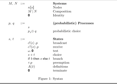
M, N ::= Systems
nJsK Nodes
M|N Composition
0 Identity
p, q ::= (probabilistic) Processes
s
pp⊕q probabilistic choice
s, t ::= States
c!hei.p broadcast c?(x).p receive
ω.0 test
s+t choice
ifbthenselset branch
τ.p preemption
A(˜x) definitions
[image:9.612.138.522.115.391.2]0 terminate
Figure 1: Syntax
The syntax of our calculus is presented in Section 3.1; here we also give some basic examples of wireless networks. In Section 3.2 we formalise how networks evolve by intro-ducing an intensional semantics for our calculus; finally we prove some basic properties of our calculus in Section 3.3.
3.1. Syntax. The calculus we present is designed to model broadcast systems, particularly wireless networks, at a high level. We do not deal with low level issues, such as collisions of broadcast messages or multiplexing mechanisms [35]; instead, we assume that network nodes use protocols at the MAC level [20] to achieve a reliable communication between nodes.
Basically, the language will contain both primitives for sending and receiving messages and will enjoy the following features:
(i) communication can be obtained through the use of different channels; although the physical medium for exchanging messages in wireless networks is unique, it is rea-sonable to assume that network nodes use some multiple access technique, such as TDMA or FDMA[35], to setup and communicate through virtual channels,
(ii) communication is broadcast; whenever a node in a given network sends a message, it can be detected by all nodes in its range of transmission,
m
n i
e
o1
o2
m
n i
e
k
o1
o2
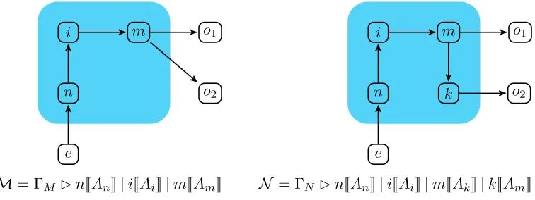
[image:10.612.120.498.118.260.2]M= ΓM ✄nJAnK|iJAiK|mJAmK N = ΓN ✄nJAnK|iJAiK|mJAkK|kJAmK
Figure 2: Example networks
The language for system terms, ranged over by M, N,· · · is given in Figure 1. Basically a system consists of a collection of named nodes at each of which there is some running code. The syntax for this code is a fairly straightforward instance of a standard process calculus, augmented by a probabilistic choice; code descriptions have the usual constructs for channel based communication, with inputc?(x).pbeing the unique binder. This gives rise to the standard notions of alpha-conversion, free and bound occurrences of variables in system terms and closed system terms.
We only consider the sub-language of well-formed system terms in which all node names have at most one occurrence. We use sSys to range over all closed well-formed terms. A (well-formed) system term can be viewed as a mapping that assigns to node names the code they are executing. A sub-term nJsK appearing in a system term M represents node n running codes. In the following we make use of standard conventions; we omit trailing occurrences of 0and we useQni=1miJsiKto denote the system termm1Js1K| · · · |mnJsnK.
Additional information such as the connectivity between nodes of a network is needed to formalise communications between nodes. Network connectivity is represented by a graph Γ =hΓV ,ΓEi; here ΓV is a finite set of nodes and ΓE ⊆(ΓV ×ΓV) is an irreflexive relation
between nodes in ΓV. Intuitively, (m, n) ∈ΓE models the possibility for node n to detect
broadcasts fired bym.
We use the more graphic notation Γ⊢v to mean v∈ΓV and Γ⊢m→n for (m, n)∈
ΓE. Similarly we use Γ ⊢ n ← m to denote Γ ⊢ m → n. Sometimes we also use the
notations Γ⊢m↔nfor{(n, m),(m, n)} ⊆ΓE and Γ⊢m⇄nto denote either Γ⊢m→n
or Γ⊢m←n.
Anetwork consists of a pair (Γ✄M), representing the system M, fromsSys, executing relative to the connectivity graph Γ. All nodes occurring in M, nodes(M), will appear in Γ and the effect of running the code atn∈nodes(M) will depend on the connectivity ofn in Γ. But in general there will be nodes in Γ which do not occur in M; let Intf(Γ✄M) = ΓV \nodes(M); we call this set the interface of the network Γ✄M, and its elements are
calledexternal nodes. Intuitively these are nodes which may be used to compose the network Γ✄M with other networks, or to place code for testing the behaviour of M.
Example 3.1. Consider M described in Figure 2. There are six nodes, three occupied by code n, iand m, and three in the interfaceIntf(M) , e, o1 and o2. Here, and in future examples, we differentiate between the interface and the occupied (internal) nodes using shading. Suppose the code at nodes is given by
An⇐c?(x).d!hxi.0 Ai ⇐d?(x).d!hf(x)i.0 Am⇐d?(x).(d!hxi.00.8⊕ 0)
Then M can receive input from node e at its interface along the channelc; this is passed on to the internal node i using channel d, where it is transformed in some way, described by the function f1, and then forwarded to node m, where 80% of the time it is broadcast to the external nodeso1 and o2. The remainder of the time the message is lost.
The networkN has the same interface asM, but has an extra internal nodekconnected too2, andm is only connected to one interface nodeo1 and the internal nodek. The nodes iand nhave the same code running as in M, while nodesm and kwill run the code
Ak⇐d?(x).(d!hxi.00.9⊕0)
Intuitively, the behaviour of N is more complex than that of M; indeed, there is the possibility for a computation ofN to deliver a value only to one between the external nodes o1 and o2, while this is not possible in N. However, 81% of the times this message will be delivered to both these nodes, and thus it is more reliable than M. Suppose now that we change the code at the intermediate node m inM,
M1 = ΓM✄. . .|mJBmK where Bm⇐d?(x).(τ.(d!hxi.00.5⊕0) +τ.d!hxi.0)
InM1the behaviour at the nodemis non-deterministic; it may act like a perfect forwarder, or one which is only 50% reliable. Optimistically it could be more reliable than M, or pessimistically it could be less reliable than the latter. Further, there is no possibility for the network M1 to forward the message to only one of the external nodeso1,o2, so that its behaviour is somewhat less complex than that ofN.
As a further variation letM2 be the result of replacing the code at m with
Cm ⇐d?(x).D
D⇐τ.(d!hxi.00.5⊕ τ.D)
Here the behaviour is once more deterministic, with the probability that the message will be eventually transmitted successfully through node k approaching 1 in the limit. Thus, this network is as reliable asM1, when the latter is viewed optimistically.
3.2. Intensional Semantics. We now turn our attention on the operational semantics of networks. Following [7], processes will be interpreted as probability distributions of states; such an interpretation is encoded by the functionP(·) defined below:
P(s) = s
P(p1p⊕p2) = p·P(p1) +(1−p)·P(p2).
(s-Snd)
c!hei.pc−→!JeKP(p)
(s-Rcv)
c?(x).p−→c?v P(p{v/x})
(s-τ)
τ.p−→τ P(p)
(s-Suml) s−→α ∆ s+t−→α ∆
(s-SumR) t−→α ∆ s+t−→α ∆
(s-then) s−→α ∆
ifbthenselset−→α ∆ JbK= true
(s-else) t−→α ∆
ifbthenselset−→α ∆ JbK= false
(s-Call) s{˜e/˜x}−→µ ∆
A(e)e −→µ ∆ A(˜x)⇐s
Figure 3: Pre-semantics of states
Sometimes we will need to consider the probability distribution associated to system terms; this is done by letting
P(0) = 0
P(nJpK) = nJP(p)K
P(M1|M2) = P(M1)|P(M2)
wherenJP(p)Krepresents a distribution over sSys, obtained by a direct application of
Equa-tion (2.1) to the funcEqua-tionnJ·K which maps states into system terms. Similarly, P(M1|M2)
is obtained by applying Equation (2.2) to the function (· | ·) :sSys×sSys→sSys.
The intensional semantics of networks is defined incrementally. We first define a pre-semantics for states, which is then used for giving the judgements of (state based) networks.
The pre-semantics for states takes the form
s−→α ∆
wheresis a closed state, that is containing no free occurrences of a variable, ∆ is a distribu-tion of states andµcan take one of the formsc!v, c?vorτ. The deductive rules for inferring these judgements are given in Figure 3 and should be self-explanatory. It assumes some mechanism for evaluating closed data-expressionseto values JeK. Note that we assume that definitions have the formA(˜x)⇐s, wheresis a state; this is because actions for definitions are inherited by the state that is associated to them, and judgements are not defined for (probabilistic) processes. Also, note that we have a special state ω for which no rule has been defined. The role of this construct will become clear in Section 4.
Judgements in the intensional semantics of networks take the form Γ✄M−→µ ∆
where Γ is a network connectivity, M is a system from sSys, and ∆ is a distribution over
(b-broad) s−→c!v ∆
Γ✄nJsKn.c−→!vnJ∆K
(b-rec) s−→c?v ∆
Γ✄nJsKm.c−→?vnJ∆K
Γ⊢m→n
(b-deaf)
s6−−→c?v
Γ✄nJsKm.c−→?vnJsK
(b-disc)
Γ✄nJsKm.c−→?vnJsK
Γ⊢m6→n
(b-0)
0m.c−→?v0
(b-τ) s−→τ p
Γ✄nJsK−→n.τ nJ∆K
P(p) = ∆
(b-τ.prop) Γ✄M−→n.τ ∆
Γ✄M|N −→n.τ ∆|N
(b-prop)
Γ✄Mm.c−→?v∆, Γ✄N m.c−→?vΘ
Γ✄M|N m.c−→?v∆|Θ
(b-sync)
Γ✄Mm.c−→!v∆, Γ✄Nm.c−→?vΘ
[image:13.612.95.526.111.372.2]Γ✄M|N m.c−→!v∆|Θ
Figure 4: Intensional semantics of networks
actionµ, and with probability ∆(N) be transformed into the systemN, for everyN ∈ ⌈∆⌉. The action labels can take the form
(i) receive, n.c?v, meaning that the value v is detected on channel c by all nodes in nodes(M) which are reachable fromnin Γ,
(ii) broadcast, n.c!v: meaning the node n (occurring in nodes(M), and therefore in Γ) broadcasts the value v on channelc to all nodes directly connected to nin Γ
(iii) internal activity, n.τ, meaning some internal activity performed by noden.
The rules for inferring judgements are given in Figure 4. Here we have omitted the sym-metric counterparts of rules (b-Sync) and (b-TauProp). Rule (b-broad) models the
capability for a node to broadcast a value v through channelc, assuming the code running there is capable of broadcasting along c. Here the distribution ∆ is in turn obtained from the residual of the statesafter the broadcast action.
Example 3.2. Consider the simple network Γ✄nJsKwhere Γ is an arbitrary connectivity graph and the codeshas the form c!hvi.(s11/4⊕s2).
The pre-semantics of states determines thats−→c!v P(s11/4⊕s2) =1/4·s1+3/4·s2, using Rule (b-Snd) Thus according to the rule (b-broad) we have the judgement
Γ✄nJsK n.c−→!v 1
4·nJs1K+ 3
4 ·nJs2K
Rules (b-rec),(b-deaf) and (b-disc) express how a node reacts when a message is
broadcast a message, or it is not in the range of transmission of the sender; In both cases this node cannot detect the transmission at all.
The rules (b-τ) and (b-τ.prop) model internal activities performed by some node of
a system term; the latter (together with its symmetric counterpart) expresses the inability for a node which performs an internal activity to affect other nodes in a system term. Here again, ∆|Θ is a distribution over sSys, this time obtained by instantiating Equation (2.2) to the function (· | ·) :sSys×sSys→sSys.
Finally, rules (b-sync) and (b-prop) describe how communication between nodes of a
network is handled; here the result of a synchronisation between an output and an input is again an output, thus modelling broadcast communication [28].
3.3. Properties of the Calculus. We conclude this section by summarising the main properties enjoyed by the intensional semantics of our calculus.
Here (and in the rest of the paper) it will be convenient to identify networks and distributions of networks up to a structural congruence relation ≡. This is first defined for states as the smallest equivalence relation which is a commutative monoid with respect to + and 0, and which satisfies the equations if b then s else t ≡ s if JbK = true,
if b then selse t≡ t if JbK= false and A(˜e) ≡ s{˜e/˜x} if A(˜x) ⇐ s. For system terms, we let ≡ be the smallest equivalence relation which is a commutative monoid with respect to (· | ·) and 0, and which satisfies the equation s ≡t implies mJsK≡ mJtKfor any node m. Finally, we let (ΓM✄M)≡(ΓN✄N) iff Γ1= Γ2andM ≡N. Structural congruence is also defined for distributions of networks via the lifted relation≡e. With an abuse of notation,
the latter is still denoted as ≡.
The properties that we prove in this section give an explicit form to the structure of a network (Γ✄M) and a distribution ∆ in the case that an action (Γ✄M)−→µ ∆ can be inferred in the intensional semantics presented in Section 3.2.
Proposition 3.3(Tau-actions). Let Γ✄M be a network; then Γ✄M−→m.τ ∆if and only if (i) M ≡mJ(τ.p) +sK|N,
(ii) ∆≡P(mJpK)|N
Outline of the Proof. We first need to prove a similar statement for states. Lettbe a state; thent−→τ Θ if and only ift≡τ.p+sfor somep, ssuch thatP(p) = Θ. The two implications
of this statement are proved separately.
To prove Proposition 3.3 suppose first that Γ✄M−→m.τ ∆ for some distribution ∆. We show thatM ≡mJτ.p+sK|N, ∆≡P(mJpK)|N by structural induction on the proof of the
derivation above.
If the last rule applied is (b-τ), thenM =mJtKfor sometsuch thatt−→τ Θ , ∆ =mJΘK.
Since t−→τ Θ then t≡τ.p+sfor some processp such thatP(p) = Θ, which also gives
∆ = P(mJpK). By definition of structural congruence M ≡ mJτ.p+sK ≡ mJτ.p+sK|0.
Further, ∆≡P(mJpK)|0, and there is nothing left to prove.
If the last rule applied is (b-τ.prop), thenM ≡N|Lfor someN, Lsuch thatN−→m.τ∆N;
further, ∆ = ∆N |L. By inductive hypothesis we have that N ≡ mJτ.p+sK|N′ and
∆N ≡ P(mJpK)|N′. By performing some simple calculations we find that M ≡ N |L ≡
mJτ.p+sK|(N′|L) and ∆≡∆N |L≡P(mJpK)|(N′|L)≡P(mJpK)|(N′|L).
Proposition 3.4 (Input). For any network Γ✄M we have that Γ✄Mm.c−→?v∆iff (i) m /∈nodes(M),
(ii) M ≡Qi∈IniJ(c?(x).pi) +siK|Qj∈JnjJsjK,
(iii) for any i∈I, Γ⊢m→ni,
(iv) for any j∈J, either Γ⊢m6→nj or sj c?v
−→6 , (v) ∆≡P(Qi
∈IniJpi{v/x}K)|Qj∈JnjJsjK.
Proposition 3.5 (Broadcast). Let Γ✄M be a network; thenΓ✄Mm.c−→!v∆for some ∆iff (i) M ≡mJ(c!hei.p+s)K|N, where JeK=v,
(ii) Γ✄Nm.c−→?vΘ, (iii) ∆≡P(mJpK)|Θ.
An immediate consequence of the results above is that actions in the intensional semantics are preserved by structurally congruent networks.
Corollary 3.6. Let M,N be two networks such that M ≡ N. If M−→µ ∆then N −→µ Θ for some Θ such that∆≡Θ.
Another trivial consequence that follows from the results above is that the intensional semantics does not change the structure of a network.
Definition 3.7 (Stable distributions). A (node)-stable sub-distribution ∆∈ Dsub(sSys) is
one for which wheneverM, N ∈ ⌈∆⌉ it follows that nodes(M) = nodes(N). A distribution over networks is said to be (node)-stable if it has the form Γ✄∆, and ∆ is a stable sub-distribution inDsub(sSys).
Corollary 3.8. Whenever Γ✄M −→µ ∆ then ∆is node-stable; further, for any N ∈ ⌈∆⌉ we have that nodes(M) =nodes(N).
4. Compositional Reasoning for Networks
The aim of this Section is to develop preorders of the form
M❁
∼behav N (4.1)
Intuitively this means that the networkMcan be replaced byN, as a part of a larger overall network, without any loss of behaviour. The intention is that the internal structure of the networks M, N should play no role in this comparison; the names used to identify their internal stations and the their communication topology should not be important. Intuitively the only behaviour to be taken into account in this extensional comparison is the reception of values at the their interface, the values subsequently broadcast at the interface.
To formalise this concept we need to say how networks are composed to form larger networks. In Section 4.1 we propose a specific composition operator,k>for this purpose, and briefly discuss its properties. We then use this operator in Section 4.2 to say how network behaviour is determined. In Section 4.3, we give the formal definition of the behavioural preorders, in a relatively standard manner following [27]; this section also treats some examples. The nature of these preorders depends on our particular choice of composition operator k>. In Section 4.4 we return to this point and offer a justification for our choice; this section may be safely ignored by the reader who is uninterested in this subtlety.
m
o1
o2
m
o1
o2
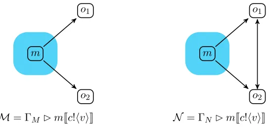
[image:16.612.173.445.116.245.2]M= ΓM ✄mJc!hviK N = ΓN ✄mJc!hviK
Figure 5: A well-formed and an ill-formed network
structure of N,M. But equally well N,M should not be able to make any assumptions about the topology of their external environment.
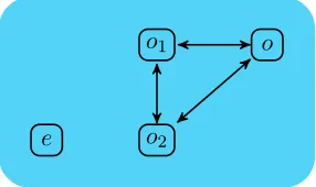
Example 4.1. Consider the networks M and N depicted in Figure 5. At least intu-itively the extensional behaviour of these two networks is the same: a broadcast of value v along channel c can be detected by the external nodes o1 and o2. However N makes an assumption about the external environment, namely that there is a connection between the external nodes o1 and o2. This slight difference can be exploited to distinguish be-tween them behaviourally. Suppose that we place the code c?(x).c!hwi at node o1 and the codec?(x).c?(y).ωat node o2 to test the behaviour of both networks. In practice, let T =o1Jc?(x).c!hwiK|o2Jc?(x).c?(y).ωK, and consider the networksM′ = ΓM✄mJc!hviK|T
andN′ = Γ
N✄mJc!hviK|T. In the first network the nodeo2 can detect both the broadcast fired by node m and node o1, leading to a state in which the special action ω is enabled. However, the same is not possible in N′, since there is no connection between the external nodes o1 and o2. That is, node o2 can only detect the broadcast fired by node m, ending in a state in which the special actionω remains guarded by an input. As we will see later, the clauseω plays a crucial role in distinguishing networks.
The problem in Example 4.1 is caused by the presence of a connection between the two external nodes in the network N of Figure 5; intuitively this represents an assumption of N about its external environment. To avoid this problem, we focus on a specific class of networks in which connections between external nodes are not allowed. Also, we require external nodes to have at least a connection with some internal node.
Definition 4.2 (Well-Formed Networks). A networkMis well-formed iff (i) wheneverM ⊢m⇄nthen either m∈nodes(M) or n∈nodes(M), (ii) wheneverM ⊢m and M ⊢m⇄n for non∈(M)V, thenm∈nodes(M).
Henceforth we will only focus on well-formed networks, unless stated otherwise. We denote the set of well-formed networks asNets.
Finally let us provide some definitions which will be useful in the sequel. Let Mbe a (well-formed) network. We say that a node i ∈ Intf(M) is an input node if M ⊢ m ← i for some m2; conversely, if a node o ∈ Intf(M) is such that Γ ⊢ m → o we say that o is an output node. If we let In(M) = {i | iis an input node inM} and Out(M) = {o|ois an output node in M}it is easy to check thatIntf(M) =In(M)∪Out(M).
4.1. Composing Networks. One use of composition operators is to enable compositional reasoning. For example the task of establishing
N1 ❁∼behav N2 (4.2) can be simplified if we can discover a common component, that is some N such thatN1= M19N andN2 =M29N for some composition operator9; then (4.2) can be reduced to establishing
M1❁∼behav M2, assuming that the behavioural preorder in question, ❁
∼behav, is preserved by the composition operator 9.
However another use of a composition operator is in the definition of the behavioural preorder ❁
∼behav itself. Intuitively we can define
N1 ❁∼behav N2 (4.3) to be true if for every component T which can be composed with both N1 and N2, the external observable behaviour of the composite networksN19T and N29T are related in some appropriate way. T is a testing network which is probing N1 and N2 for behavioural differences, along the lines used informally in Example 4.1. Intuitively this should be black-box testing, in which the tester, namely T, should have no access to the internal stations of the networks being tested, namely N1 and N2. All it can do is place code at their external interfaces, to transmit values and examine the subsequent effects, as seen again at the interfaces.
Definition 4.3(Composing networks). For any two networksM= ΓM✄MandP = ΓP✄P
let M k>P be given by:
(ΓM✄M)k>(ΓP ✄P) = (
(ΓM∪ΓP)✄(M |P), if nodes(M)∩(P)V =∅
undefined, otherwise
The composed connectivity graph ΓM∪ΓP is defined by letting (ΓM∪ΓP)V = (ΓM)V∪(ΓP)V
and (ΓM ∪ΓN)E = (ΓM)E ∪(ΓP)E.
The intuition here is that the composed network M k>P is constructed by extending the network under test,M, allowing code to be placed at its interface, and allowing completely fresh stations to be added. These fresh stations can be used by the tester to compute the results of probes made on M.
Proposition 4.4. Suppose M,N,P ∈Nets. Then (1) M k>P ∈Nets, whenever it is defined
(2) (M k>N)k>P =M k>(N k>P), whenever both are defined
m
o1
o2
o1
e
o2
m
o1
o2
e
[image:18.612.129.489.118.273.2]M N (M k>N)
Figure 6: Network composition viak>
There is an inherent asymmetry in the definition of our composition operator; inM k>P we allow P to place code at the interface nodes ofMbut not the converse. As a result the operator is not in general symmetric, as can be seen from Example 4.5.
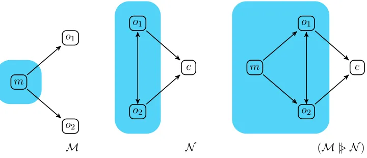
Example 4.5 (k> is asymmetric). Let M,N be the networks depicted in Figure 6. Here the network M k>N is well-defined and depicted on the right of Figure 6. Intuitively, this is the network obtained by extendingMwith the information provided byN; these include the code running at nodeso1, o2, a connection between such nodes, and a connection from o1, o2, respectively, to a fresh nodee, whose running code is left unspecified. The network M k> N is well-defined because none of the connections specified in N involve the node m∈nodes(M); that is, when extendingMwithN it is ensured that the latter can interact with the nodem only via the nodeso1, o2.
On the other hand, the composition N k> M is not defined. Intuitively, in N nodes o1 ando2 can interact with the external environment only via the external nodee. This is in contrast with the definition of M, where node m can be used to broadcast messages to such nodes.
One might wonder if a symmetric composition operator could be used in place of our k
>; this point is discussed at length in Section 4.4. Neverthelessk>is a natural operator, and the next result shows that it can be used to construct all non-degenerate networks starting from single nodes. Let Gbe the collection of networks which contain exactly one occupied
node, that isG={(Γ✄G)|G≡mJsKfor some s, m}.
Proposition 4.6. SupposeM ∈Netsis a network such that nodes(M)is not empty. Then M ≡ N k>G for someN ∈Nets and G ∈G.
Proof. See Appendix A, Page 61.
We use the termgenerating networks to refer to elements of G. The import of Proposition
4.2. Testing Structures. The introduction of the composition operator k>allows the de-velopment of a behavioural theory based on a probabilistic generalisation of theDe Nicola and Hennessy testing preorders [27]. In order to develop such a framework, we will exploit the mathematical tools introduced in Section 2; our aim is to be able to relate networks with different connection topologies.
In our framework, as has already been indicated, testing can be summarised as follows: the network to be tested is composed with another one, usually called a testing network. The composition of these two networks is then isolated from the external environment, in the sense that no external agent (in our case nodes in the interface of the composed network) can interfere with its behaviour; we will shortly present how such a task can be accomplished. The composition of the two networks isolated from the external environment takes the name ofexperiment.
Once these two operations (composition with a test and isolation from the external environment) have been performed, the behaviour of the resulting experiment is analysed to check whether there exists a computation that yields a state which is successful. This task can be accomplished by relying on testing structures, which will be presented shortly. At an informal level, successful states in our language coincide with those associated with networks where at least the code running at one node has the specialaction ωenabled. Since networks have probabilistic behaviour, each computation will be associated with the probability of reaching a successful state; thus, every experiment will be associated with a set of success probabilities, by quantifying over all its computation.
Let us now look at how the procedure explained above can be formalised; the topic of composing networks has already been addressed in detail in Section 4.1, in which we defined the operatork>and proved basic properties for it. To model experiments and their behaviour, we rely on the following mathematical structure.
Definition 4.7. ATesting Structure (TS) is a triplehS,_, ωi where (i) S is a set of states,
(ii) the relation _is a subset of S× D(S),
(iii) ω is a success predicate over S, that isω :S→ {true,false}.
Testing structures can be seen as (degenerate) pLTSs where the only possible action cor-responds to the internal activity τ, and the transition −→τ is defined to coincide with the reduction relation _. Conversely every pLTS automatically determines a testing structure, by concentrating on the relation −→.τ
Our goal is to turn a network into a testing structure. This amounts to defining, for networks, a reduction relation and the success predicate ω. As we have mentioned in the beginning of this section, when converting a network into a testing structure, we want to make it isolated from the external environment.
When considering simpler process languages, like CCS or CSP (and, more generally, their probabilistic counterparts), processes are converted into testing structures by identi-fying the reduction relation with the internal activity τ; that is, processes are not allowed to synchronise with some external agent via a visible action.
On the other hand, input actions always originate from non-internal nodes. Hence they can be seen as external activities which can influence the behaviour of a network. Therefore, input actions should not be included in the definition of the reduction relation for networks. Finally, the success predicateωis defined to be true for exactly those networks in which the success clauseω is enabled in at least one node.
Example 4.8. The main example of a TS is given by hNets,_, ωi where
(i) (Γ✄M)_(Γ✄∆) whenever
(a) Γ✄M−→m.τ ∆ for somem∈nodes(M)
(b) or, Γ✄Mm.c−→!v∆ for some value v, node name mand channel c (ii)
ω(M) =
(
true, if M ≡M′|nJω+sK, for somes, n, M′
false, otherwise
If ω(M) = true for some system term M, we say that a network Γ✄M, where Γ is an arbitrary connectivity graph, isω-successful, or simply successful. Note that when recording an ω-success we do not take into account the node involved.
As TSs can be seen as pLTSs, we can use in an arbitrary TS the various constructions intro-duced in Section 2. Thus the reduction relation _can be lifted to Dsub(sSys)× Dsub(sSys)
and we can make use of the concepts of hyper-derivatives and extreme-derivatives, intro-duced in Section 2, to model fragments of executions and maximal executions of a testing structure, respectively. Hyper-derivations in testing structures are denoted with the symbol ==✄, while we use the symbol ==✄≻for extreme derivations.
Below we provide two simple examples that show how to reason about the behaviour of the testing structures presented in Example 4.8.
Example 4.9. Consider the testing structure associated with the networkN in the center of Figure 11, where the codeq is given by the definitionq ⇐q0.5⊕c!hvi.0. We can show that,
in the long run, this network will broadcast messagevto the external locationoby exhibiting a hyper derivation for it which terminates in the point distribution ΓN ✄kJc!hvi.0K. If we
let N1 denote the configuration ΓN ✄kJc!hvi.0K, we have the following hyper-derivation:
N = 12 · N + 12 · N1
1
2 · N _ 212 · N + 212 · N1 ..
. 1
2n · N _ 2n1+1 · N + 2n1+1 · N1 ..
.
Let ∆′ = P∞n=1 21n · N1. It is straightforward to check that ∆′ = N1 and therefore we have the hyper-derivation N ==✄ N1.
Executions, or maximal computations, correspond to extreme derivatives in the test-ing structure associated with (N k> T), as defined in Section 2. Since the framework is probabilistic, each execution (that is extreme derivative) will be associated with a proba-bility value, representing the probaproba-bility that it will lead to anω-successful state. Since the framework is also nondeterministic the possible results of this test application is given by a non-empty set of probability values.
Definition 4.10 (Tabulating results). The value of a sub-distribution in a TS is given by the functionV :Dsub(S)→[0,1], defined byV(∆) =
P
{∆(s) | ω(s) =true}. Then the set of possible results from a sub-distribution ∆ is defined byO(∆) ={ V(∆′) | ∆ ==✄≻∆′}.
Example 4.11. LetN be the network from Example 4.9 and consider the testing network T given in Figure 11, where the code is determined by t⇐c?(x).ω.0. It is easy to check that N k> T is well-defined and is equal to Γ✄kJqK|oJtK, where Γ is the connectivity graph containing the three nodes k, o, l and having the connections from Γ ⊢ k → o and Γ ⊢ o ← t. So consider the testing structure associated with it; recall that we have the definition q ⇐q0.5⊕c!hvi.0. For convenience let N1 = ΓN✄kJc!hvi.0K as in the previous example, N2 = ΓN ✄kJ0K and Tω = ΓT ✄oJω.0K. Then we have the following
hyper-derivation for N k>T:
N k>T _ (12 · N k>T +12 · N1k>T) + ε 1
2 · N k>T +12 · N1 k>T _ (212 · N k>T + 212 · N1 k>T) + 12 · N2 k>Tω
..
. ... ...
1
2n · N k>T +21n · N1k>T _ (2n1+1 · N k>T +2n1+1 · N1k>T) + 21n · N2k>Tω
..
. ... ...
were we recall that εdenotes the empty sub-distribution, that is the one with⌈ε⌉=∅. We have therefore the hyper-derivation
N k>T ==✄ε+ ∞
X
n=1 1
2nN2 k>Tω =N2 k>Tω.
Further, the above hyper-derivation satisfies the constraints required by ==✄≻ , defined in Section 2, and therefore we have the extreme derivative N k>T ==✄≻ N2k>Tω. Since V(N2 k>Tω) = 1 we can therefore deduce that 1∈ O(N k>T).
4.3. The behavioural preorders. We now combine the concepts of the previous two sections to obtain our behavioural preorders. We have seen how to associate a non-empty set of probabilities, tabulating the possible outcomes from applying the testT to the network N. As explained in [7] there are two natural ways to compare such sets, optimistically or pessimistically.
Definition 4.12 (Relating sets of outcomes). LetO1,O2 be two sets of values in [0,1]. (i) TheHoare’s Preorder is defined by lettingO1 ⊑H O2 whenever for anyp1∈ O1 there
exists p2∈ O2 such that p1 ≤p2.
o1
o2 e
o
Figure 7: A test
Given two networks M,N we can relate their behaviour, when extended with a testing network T, by comparing the success outcomes of M k> T and N k> T (provided both these networks are defined) via Definition 4.12. We can go further and consider what is the relationship between such sets of outcomes with respect to all possible tests T which can be used to extend the networks M,N.
Definition 4.13 (Testing networks). For M1,M2 ∈ Nets such that In(M1) = In(M2),
Out(M1) =Out(M2), we write
(1) M1 ⊑may M2 iff for every (testing) network T ∈ Nets such that both M1 k> T and M2 k>T are defined, O(M1 k>T)⊑H O(M2 k>T).
(2) M1 ⊑must M2 iff for every (testing network) T ∈ Nets such that bothM1 k> T and M2 k>T are defined, O(M1 k>T)⊑S O(M2 k>T)
We use M1 =may M2 as an abbreviation for M1 ⊑may M2 and M2 ⊑may M1. The relation =must is defined similarly. Finally, we say that M1 ⊑ M2 iff both M1 ⊑may M2 and M1 ⊑mustM2 hold, andM1 ≃ M2 iff M1 ⊑ M2 and M2 ⊑ M1.
Some explanation is necessary for the requirement on the interface of networks we have placed in Definition 4.13. This constraint establishes that two networksMandN are always distinguished if the sets of their input or output nodes differ. As we already mentioned, external nodes can be seen as terminals that can be accessed by the external environment to interact with the network. Roughly speaking, the constraint we have placed corresponds to the intuition that the external environment can distinguish two networks Mand N by simply looking at the terminals that it can use to interact with these two networks.
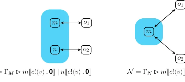
Example 4.14. Consider the testing network
T = ΓT ✄eJc!h0iK|o1Jd?(x).c!hxiK|o2Jd?(x).c!hxiK|oJc?(x).c?(y).ωK
where the connectivity is described in Figure 7. This can be used to test the networksM,N from Example 3.1 in the testing structure of Example 4.8.
Intuitively the test sends the value 0 along the channelcat the nodee, awaits for results along the channel dat the nodes o1 and o2. These results are processed at node o, where success might be announced.
The combined network (M k> T) is deterministic in this TS, although probabilistic, and so has only one extreme derivative; O(M k>T) ={0.8}.
A similar calculation shows thatO(N k>T) ={0.81}; it therefore follows thatN 6⊑may Mand M 6⊑mustN.
[image:22.612.235.378.115.200.2]m
n
o1
o2
m
o1
o2
[image:23.612.168.464.119.251.2]M= ΓM ✄mJc!hvi.0K|nJc!hvi.0K N = ΓN ✄mJc!hviK
Figure 8: Broadcast vs Multicast
The combined network (M2 k> T) is also deterministic, although it has limiting
be-haviour;O(M2k>T) ={1}. Thus, in this case we have bothO(M k>T) ⊑H O(M2k>T) and O(M1k>T) ⊑H O(M2 k>T). Further, we have that O(M1 k>T) ⊑S O(M2 k>T), butO(M2 k>T)6⊑S O(M1 k>T).
Example 4.15 (Broadcast vs Multicast). Consider the networks M and N in Figure 8. Intuitively inN the valuevis (simultaneously) broadcast to both nodeso1 and o2 while in Mthere is a multicast. More specificallyo1receivesvfrom modemwhile in an independent broadcast o2 receives it fromn.
This difference in behaviour can be detected (when we compare the networks optimisti-cally) by the testing network
T = ΓT ✄o1Jc?(x).c!hwi.0K|o2Jc?(x).c?(y).if y= 0then 0 elseωK
assumingvis different thanw; here we assume ΓT is the simple network which connectso1to o2. BothM k>T andN k>T are well-formed and note that they are both non-probabilistic. Because N simultaneously broadcasts to o1 and o2 the second value received by o2 is alwayswand therefore the test never succeeds;O(N k>T) ={0}. On the other-hand there is a possibility for the test succeeding when applied toM, 1∈ O(M k>T). This is because in M node m might first transmit v to o1 after which n transmits w to o2; now node n might transmit the value v to o2 and assuming it is different than w we reach a success state. It follows thatM 6⊑may N.
Note that we can slightly modify the testT to show that we also haveN 6⊑must N. To this end, let
T′ = ΓT ✄o1Jc?(x).c!h0i.0K|o2Jc?(x).c?(y).if y= 0thenωelse 0K
In this case we have that O(M k>T′) = {0,1}, while O(N k>T′) ={1}, and by definition O(N k>T′)6⊑
S O(M k>T′).
One might also think it possible to use the difference between broadcast and multicast to design a test T′′ for which O(N k>T′′)6⊑
H O(M k>T′′) and O(M k>T′′)6⊑SO(N k>T′′).
For example, if we let T′′ = T′ we obtain that 1 ∈ O(N k>T′). This is because because inN k>T′ the second value received byo
m
n
k o
m k o
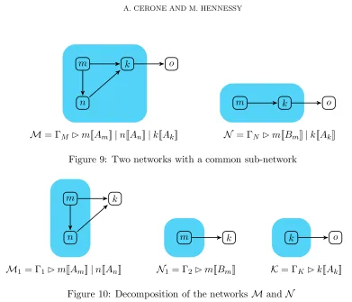
[image:24.612.103.494.70.405.2]M= ΓM ✄mJAmK|nJAnK|kJAkK N = ΓN✄mJBmK|kJAkK
Figure 9: Two networks with a common sub-network
m
n
k
m k k o
M1= Γ1✄mJAmK|nJAnK N1 = Γ2✄mJBmK K= ΓK✄kJAkK
Figure 10: Decomposition of the networksMand N
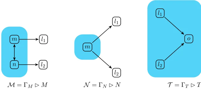
will be proved formally later as a consequence of Example 6.4 and Theorem 6.2. Similarly, Theorem 6.14 shows thatM ⊑must N.
One pleasing property of the behavioural preorders is that they allow compositional reasoning over networks.
Proposition 4.16 (Compositionality). Let M1,M2 be two networks such that M1 ⊑may M2 (M1 ⊑must M2), and let N be another network such that both (M1 k>N) and (M2k> N) are defined. Then (M1 k>N)⊑may(M2 k>N) ((M1 k>N)⊑must (M2 k>N)).
Proof. A direct consequence ofk>being both associative and interface preserving.
We end this section with an application of this compositionality result.
Example 4.17. Consider the networks M and N in Figure 9, where the codes at the various nodes are given by
Am ⇐ c!hvi.0
An ⇐ c?(x).d!hwi.0
Ak ⇐ c?(x).d?(y).e!hui.0
Bm ⇐ c!hvi.d!hwi.0
l o k o o l
M= ΓM ✄lJpK N = ΓN ✄kJqK T = ΓT ✄oJtK
Figure 11: A problem with the composition operator
4.4. Justifying the operator>k. Here we revisit Definition 4.3 and in particular investi-gate the possibility of using alternative composition operators. The remainder of the paper is independent of this section and so it may be safely skipped by the uninterested reader.
Here we take a more general approach to composition; rather than give a particular operator we discuss natural properties we would expect of such operators. Let us just pre-suppose aconsistency predicate Pon pairs of networks determining when their composition should be defined. The only requirement onMPN is that whenever it is defined the result-ing composite network is well-formed. Since the composite network should be determined by that of its components this amounts to requiring that
P(M,N) implies nodes(M)∩nodes(N) =∅ for any M,N ∈Nets (4.4)
Given a consistency predicate satisfying (4.4) we can now generalise Definition 4.3 to give a range of different composition operators.
Definition 4.18 (General composition of networks). Let Pbe a consistency predicate on networks inNetssatisfying (4.4). Then we define the associated partial composition relation by:
(ΓM ✄M)9P(ΓN✄N) = (
(ΓM ∪ΓN)✄(M|N), ifP((ΓM ✄M),(ΓN ✄N))
undefined, otherwise
The connectivity graph ΓM∪ΓN is defined as in Definition 4.3.
Example 4.19. Let Ps be the partialss binary predicate defined by letting Ps(M,N) whenever
• nodes(M)∩nodes(N) =∅
• M ⊢m→n if and only if N ⊢m→n, for everym∈nodes(M) and n∈nodes(N), • M ⊢m←n if and only if N ⊢m←n, for everym∈nodes(M) and n∈nodes(N), By definition this satisfies the requirement (4.4) above, and intuitively it only allows the composition whenever the two individual networks agree on the interconnections between internal and external nodes.
For notational convenience we denote the operator 9Ps withk. It is easy to check that
this operator is both associative and commutative.
Thus a priori this composition operator k could equally well be used to develop the testing theory in Section 4.3. Unfortunately the resulting theory would be degenerate.
However if the operatork is used to combine a test with the network being observed they are indistinguishable.
This is because if there is a network T such thatM k T and N k T are well-defined then o can not be in nodes(T). For if o were in nodes(T), then since M ⊢ l → o the definition of the operator implies that T ⊢ l → o. This in turn implies that N ⊢ l → o, which is not true.
Now since no testing network which can be applied to both M and N can place any code at o, no difference can be discovered between them.
The question now naturally arises about which consistency predicate Plead to reason-able composition operators9Ps, in the sense that at least the resulting testing theories are
not degenerate. We want to be able to compare networks with different connectivity graphs, and possibly different nodes, such as M and N in Figure 11. We also should not be able to change the connectivity of the internal nodes of a network when we test it; we wish to implement black-box testing, where the nodes containing running code cannot be accessed directly.
These informal requirements can be formulated as natural requirements on composition operators. The first says that the composed network is completely determined by the components:
(I) Merge: the operator9should be determined by some predicatePusing Definition 4.3. Intuitively the interface of a network is how their external behaviour is to be observed. Since our aim is to enable compositional reasoning over networks, we would expect compo-sition to preserve interfaces:
(II) Interface preservation: If In(M) =In(N), Out(M) =Out(N) andT can be com-posed with both, that is both M9T and N 9T are well-defined, then In(M9T) =
In(N 9T), Out(M9T) =Out(N 9T).
The final requirement captures the intuitive idea that reorganising the internal structure of a network should not affect the ability to perform a test; in fact the reorganisation is simply a renaming of nodes. Letσ be a permutation of node names. We use (Γ✄M)σ to denote the result of applyingσ to the node names in M and in the connectivity graph Γ. (III) Renaming: SupposeM9T is defined. ThenMσ9T is also defined, provided σ is
a node permutation which satisfies • σ(e) =e for everye∈Intf(M)
• no n∈nodes(T) appears in the range of σ; that is n∈nodes(T) implies σ(n) =n. Example 4.21. The operator k does not satisfy (III), as can be seen using the simple networks in Figure 11;M k T is obviously well-defined. However, consider the renamingσ which swaps node names l to k, which is valid with respect to T; the network Mσ k T is not defined, as ΓT 6⊢k→o. A slight modification will demonstrate that interfaces are also
not preserved by this operator.
Proposition 4.22. Suppose 9 satisfies the conditions (I) - (III) above. Then nodes(M)∩
Intf(N) =∅ whenever M9N is defined.
Proof. By contradiction; letM = ΓM ✄M and N = ΓN ✄N. Assume that m is a node
(2) N ⊢m,
(3) Intf(M) =Intf(Mσ). (4) m /∈Intf(M9N).
For proving the last statement just note that m ∈ nodes(M) by hypothesis, hence m ∈ nodes(M9N). By definition of interface it follows thatm /∈Intf(M9N).
Let l be a node which is not contained in ΓM, nor in ΓN. Consider the permutation
σ which swaps nodes m and l; that is σ(m) = l, σ(l) = m and σ(k) = k for all k 6= m, l. SinceM 6⊢lwe also have thatl /∈nodes(M), so thatσ(l) =m /∈nodes(Mσ). Further, the permutation σ is consistent with condition (III), renaming, when applied to networks M and N; thereforeMσ9N is defined.
Since m /∈ nodes(Mσ), by (1) above it follows that m /∈ nodes(Mσ9N); by (2), we obtain that (ΓM)σ∪ΓN ⊢m. These two statements ensure that m∈Intf(Mσ9N).
As a direct consequence of (3) and condition (II), interface preservation, we also have that m∈Intf(M9N), but this contradicts (4).
Corollary 4.23. Let9be any symmetric composition operator which satisfies the conditions (I) - (III). Suppose M19M2 is well-defined, and of the form Γ✄M. Then Γ⊢m1 6⇄m2 whenever mi∈nodes(Mi).
Proof. A simple consequence of the previous result.
What this means is that if we use such a symmetric operator when applying a test to a network, as in Definition 4.7, then the resulting testing preorder will be degenerate; it will not distinguish between any pair of nets. In some sense this result is unsurprising. For T to test M in M9T it must have code running at the interface of M. But, as we have seen, condition (III) more or less forbidsT to have code running at the interface ofM.
Thus we have ruled out the possibility of basing our testing theory on a symmetric composition operator. The question now remains what composition operator is the most appropriate? We have already stated that conditions (I)-(III) are natural, and since there are no further obvious requirements we could choose the operator with greatest expressive power among those that satisfy conditions (I)-(III). Here an operator9P1 is more expressive than another 9P2 if, whenever M9P1 N is defined for any two arbitrary networks M,N,
then so is M9P2 N, and the result of the two compositions above is the same. The next
Lemma shows that the operator which we are looking for is exactlyk>.
Lemma 4.24. Let Pbe any consistency predicate satisfying (4.4) above. Then if M9PN is defined so is M k>N and moreover M9PN = M k>N.
Proof. Obvious from the definition of k>in Definition 4.3.
5. Extensional Semantics