An efficient and high-resolution topology optimization method based
on convolutional neural networks
Liang Xue1,2, Jie Liu2, Guilin Wen1,2*, Hongxin Wang1
1. State Key Laboratory of Advanced Design and Manufacturing for Vehicle Body, Hunan University, Changsha 410082, Peoples Republic of China
2. Center for Research on Leading Technology of Special Equipment, School of Mechanical and Electric Engineering, Guangzhou University, Guangzhou 510006, Peoples Republic of China
Corresponding author:
Tel.: +86 731 88823929; Fax: +86 731 88822051 Email: [email protected] (Guilin Wen)
Abstract:
Topology optimization is a pioneering design method that can provide various candidates with high mechanical properties. However, the high-resolution for the optimum structures is highly desired, normally in turn leading to computationally intractable puzzle, especially for the famous Solid Isotropic Material with Penalization (SIMP) method. In this paper, an efficient and high-resolution topology optimization method is proposed based on the Super-Resolution Convolutional Neural Network (SRCNN) technique in the framework of SIMP. The SRCNN includes four processes, i.e. refining, path extraction & representation, non-linear mapping, and reconstruction. The high computational efficiency is achieved by a pooling strategy, which can balance the number of finite element analysis (FEA) and the output mesh in optimization process. To further reduce the high computational cost of 3D topology optimization problems, a combined treatment method using 2D SRCNN is built as another speeding-up strategy. A number of typical examples justify that the high-resolution topology optimization method adopting SRCNN has excellent applicability and high efficiency for 2D and 3D problems with arbitrary boundary conditions, any design domain shape, and varied load.
Keywords: Topology optimization; convolutional neural network; high-resolution
1 Introduction
The work of Bendsøe and Kikuchi (1988) plays a vital role in the development of topology optimization, followed by a number of excellent topological optimization methods to solve material distribution problems under given goals and constraints, e.g. SIMP (Bendsøe 1989; Rozvany et al. 1992; Sigmund 2001), Evolutionary Structural Optimization (ESO)/Bi-directional Evolutionary Structural Optimization (BESO) (Xie and Steven 1993; Querin et al. 1998; Huang and Xie 2007; Rozvany 2009), level-set (Wang et al. 2003; Wei et al. 2018)method, Moving Morphable Components/ Void (MMC/V) (Guo et al. 2014; Zhang et al. 2017; Lei et al. 2019), and so on. As topology optimization approaches mature and gradually shift from mathematical theory to practical engineering applications (Zhu et al. 2015), there is a growing desire for developing existed topological optimization method to hold the capacity for dealing with large-scale, e.g. buildings, aerospace (Zhu et al. 2015; Chin and Kennedy 2016; Liu et al. 2019) or high-precision, e.g. bionic bones (Sutradhar et al. 2016), convection radiators (Alexandersen et al. 2016), etc.) structures. All these structural designs are in desire need for having detail features, i.e. high-resolution, which will lead to prohibitively computational cost, especially for element-based topology optimization methods, therefore restricting the application of these methods.
A number of articles have explored the route to improve the resolution of topology optimization designs, and proposed a variety of methods with acceptable computational efficiency. For the density-based topology optimization method, there are mainly the following mainstream processing methods.
(1)Designing microstructure of elements: Groen and Sigmund(2018) and Wu et al. (2019) used the homogenization method to design the microstructure, while Zhu et al. (2017) utilized the pre-designed microstructure for topology optimization. This method does improve the resolution final layouts, but it failed to change the jagged boundaries brought by the coarse element.
(2)Adaptive adjustment of discretized mesh: For the tetrahedral mesh, Christiansen et al. (2015) moved the cell nodes to obtain a satisfactory model. Later, Wang et al. (2019a) extended the method to the case with hexahedral meshes. This is a low-cost and high-efficient post-processing method, which is easy to implement in common CAD/CAE software, However, this method is severely dependent on the mesh. In addition, the quality of the final configuration relies on the selected node adjustment criteria.
that FEA takes lot of time in the optimization. On the other hand, there are some studies that choose to increase the resolution of the design variable mesh and maintain a coarser finite element mesh. Based on the work of Nguyen (2010), the high-order finite elements were used to improve the accuracy and efficiency of the algorithm (Groen et al. 2017). An adaptive refinement/coarsening criterion was used to further accelerate the multi-resolution topology optimization method (Gupta et al. 2018). In addition, the isogeometric analysis method was utilized to map the design variables and the finite element mesh (Lieu and Lee 2017; Xu et al. 2019). Most recently, our group have proposed a novel high-resolution topology optimization method in the framework of BESO and with the use of XFEM (Wang et al. 2019b). In this method, we only refined the design variable mesh with a small cost of FEA but the error caused by the coarse finite element mesh cannot be avoided.
(4)Adaptive refinement of mesh:Kim and Yoon (2000) used this idea to continuously improve the mesh resolution during the optimization process, which can reduce initial calculation amount. Stainko (2006) improved the method by increasing the mesh resolution only for the boundary. Recently, Liao et al. (2019) designed a partial update rule that it concentrated all computational power on the elements where the model was prone to change.
The above excellent research studies can make some contributions at the algorithmic level to the goal of maximizing design resolution at the acceptable cost. Nowadays, with the rapid development of computer hardware, there are some studies that use the GPU or supercomputer to achieve the required high-resolution design (Suresh 2013; Challis et al. 2014; Aage et al. 2017). Of course, the development of algorithms and the update of hardware are not contradictory but complementary. The excellent algorithm and the efficient hardware can present more pleasing results. Referring to the development of algorithms and hardware, the author has to mention a currently very popular computer technology: machine learning. Machine learning is a kind of method for extracting implicit rules from a large amount of historical data, and its excellent generality comes from training objectives that contain implicit laws about unknown data. At present, machine learning has a wide range of applications, such as data mining, computer vision, medical diagnosis and so on (Sun 2006). Deep learning, belonging to machine learning, has become very popular in recent years due to its high efficiency, plasticity and universality.
a given mesh resolution, but requires retraining the neural network for other structures with different resolution. Li et al. (2019) implemented a set of topology optimization process without iteration using the Generative Adversarial Networks (GAN), and used another GAN as a post-processing method to improve the resolution of the final configuration.
However, the traditional multi-resolution topology optimization method normally has two shortcomings, i.e. arbitrary mapping and computational efficiency problems. It is critical to build the mapping between the FEA mesh and the design variable mesh in the multi-resolution topology optimization method. Since the mapping from low-resolution to high-resolution should be different for distinguished structural features, it is difficult to artificially design mappings for different features. Deep learning can intelligently extract structural features. In addition, in the subsequent process of extracting structural features, different structural features possess different mappings. Nonetheless, most neural networks have a fixed amount of input layer data, which will directly affect the versatility of topology optimization methods.
Therefore, this study selects the SRCNN framework (Dong et al. 2016) with better applicability to achieve the goal of enhancing the resolution of topology optimization design. Moreover, to release the computational burden in the high-resolution topology optimization method, two strategies are developed, i.e. the pooling strategy for mesh balance and a combined treatment method using 2D SRCNN. The proposed method has great versatility for 2D and 3D problems with any design domain shape, arbitrary boundary conditions, and any load cases.
The remainder of this paper is organized as follows. Section 2 describes the density-based topology optimization method. Section 3 introduces the super-resolution convolutional neural networks. Section 4 presents the implementation of the proposed methodology. Section 5 discusses the optimization results, and the conclusions are drawn in Section 6.
2 Density-based topology optimization methods
The work of this paper is done in the framework of density-based topology optimization methods. In this section, under the guidance of the classic SIMP method (Bendsøe 1989, 2009; Sigmund 2001), the mathematical description of the topology optimization problem and the entire topology optimization process will be established, forming the basis for subsequent work.
Density-based topology optimization is a method for solving the 0/1 value of the relative density
ρ
of each element in a given design domainΩ
that has been discretized into finite elements. The most classic problem is the topology optimization of the minimum structural compliance under the target volume constraints. The mathematical description of the problem is as follows:*
min min : c( ) . .: ( )
0 1
T
x x
S t V x V
x x
= ≤
< ≤ < U KU
where U and
F
are the global displacement and force vectors, respectively,K
is the global stiffness matrix,x
is the design variable, xmin is the minimum relative density, ( )V x and V* are the material volume and the target volume, respectively. The following penalty interpolation method of SIMP (Sigmund 2001) is used in the optimization process of this paper to combine the cell stiffness matrix into a global stiffness matrix.0
p i i
E =x E (2)
where Ei and E0 are the Young’s modules of element i and basic material, respectively. The penalization exponent is usually chosen as p=3 in order to push the median value of design variable closer to the 0-1 solution.
1 ( )
N i i i
E =
=
∑
K k
(3)
where N represents the total number of elements within the design domain. ki refers to the stiffness matrix of ith element. Sensitivity can be obtained by deriving the objective function to the design variables of each element. In order to ensure that the configuration always has the characteristics of mesh independence during optimization, we employed a filer scheme that proposed by Sigmund (2001). Then the optimality criteria (OC) method is used to solve this topological optimization problem. This is a classical topology optimization process. Next, we will show the basic concepts of SRCNN and how it will be implemented to the proposed topology optimization framework.
3 Super-resolution convolutional neural network (SRCNN)
The SRCNN framework of the present work, a large number of topological optimization configurations should be used as training samples, and a reasonable convolutional neural network is obtained. This section will focus on the network architecture and training process. The implementation of SRCNN combined with topology optimization will be detailed in the next section.
3.1 SRCNN
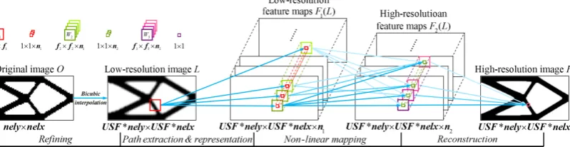
by H. The relative position and connection state of each operations are shown in Fig.1. Their structural components will be specified separately in the subsequent subsections. Refining, as a pre-processing method, is not the focus of neural networks. Therefore, its operation is no longer described separately.
Fig. 1 The relative position and connection state of SRCNN operations. nely×nelx are pixels of topology optimization design domain. USF is upscaling factor, and the selection of other parameters is
referenced from the comparative data in reference (Dong et al. 2016). (In this paper, 1 9, 1 64, 2 5, 2 32, 3 5
f = n = f = n = f = )
3.1.1 Patch extraction and representation
The main role of this part is to extract features from the low-resolution image
L
. Here, the convolution kernels are like a set of filters. Each of these filters corresponds to a feature and they are independent of each other. These features together make up the low-resolution feature maps( )
1
F L of SRCNN. The above operation can be expressed as follows:
1( ) max(0, 1 1)
F L = W L B∗ + (4)
where W1 and B1 are convolution kernels (or filter groups) and biases, respectively. In this paper, W1contains n1 convolution kernels, and their overall spatial size is f f1× 1. Each of them is independently convolved with
L
. At the same time, B1 is a vector of length n1, which corresponds one-to-one with W1 in order. It should be noted that the operator∗
represents the same type convolution operation, which needs to pa d(
f1−1 2)
circles ( f1 generally takes an odd number) on the outer side ofL
. This ensures that the dimensions of maps in next process are not reduced. Unless otherwise specified in the subsequent operations, the operator∗
defaults to the ‘same’ type convolution operation. Finally, the rectified linear unit (ReLU, max 0,(
x)
) is used as an activation function to map the calculation result to the low-resolution feature maps.3.1.2 Non-linear mapping
After the first convolution layer has extracted n1 features from the low-resolution image. The next second convolution layer maps the n1 low-resolution feature maps F L1( ) to n2
high-resolution feature maps F L2( ). SRCNN provides convolution kernels W2 of three sizes of
1 1
×
, 3 3× , and 5 5× for mapping. According to Dong et al. (2016), we select W2 with a size of 5 5× . The operational formula for this layer is expressed as follows:2( ) max(0, 2 1( ) 2)
where W2 contains n2 convolution kernels, and all of their sizes are f2× ×f n2 1. B2 is a biases vector with a length of n2. The nonlinearity of this convolutional layer is significantly strong, resulting in costing much more time to train neural networks.
3.1.3 Reconstruction
In order to get the final high-resolution configuration from the high-resolution feature map
2( )
F L , we also need a convolutional layer to reconstruct these features. Then the operation formula of the last layer is as follows:
3 2 3
min(1,max(0, ( ) ))
H = W F L B∗ + (6)
where W3 is a convolution kernel of size f3× ×f n3 2, and B3 is a biases value of size
1 1
×
. In order to match the results to the topology-optimized design variable range, modifications have been made to the ReLU activation function, as shown in Eq. 7. The reconstructed map value range is limited to between 0 and 1.( )
(
)
ReLU( ) min 1,max 0,x = x (7)
3.2 Training
With the network architecture, it is necessary to train the neural network to learn the entire process from low resolution to high resolution. Training is the process of estimating and adjusting network parameters
{
W W W B B B1, 2, 3, , , ,1 2 3}
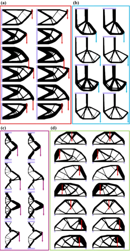
. In order to distinguish between reconstructed and real high-resolution configurations, we take different design domain sizes and employ random load positions for four classical topological optimization problems, i.e. cantilever beam (Fig. 2(a)), L-bracket (Fig. 2(b)), T-bracket (Fig. 2(c)) and MBB beam (Fig. 2(d)). A large number of high and low-resolution training samples are obtained by the traditional topology optimization method, with their corresponding initial design conditions shown in Fig. 2. It should be noted that, although only these four models are used as the base samples, this does not affect the versatility of the SRCNN architecture. It still works for any size and dimension model.With the training sample, the mean square error (MSE) is chosen as the loss function to characterize the difference between the reconstructed configuration and the real configuration:
(
)
2 11 n , ,
real
N l l N
N
Loss H L W B H
n =
=
∑
− (8)where
n
is the number of training samples selected for each iteration, the value ofl
is 1, 2 and 3, H is the high-resolution configuration of L reconstructed by SRCNN, andH
realis thehigh-resolution training sample matched with L. The random gradient descent method is used to minimize the loss value during standard backpropagation. The formula for updating each convolution kernel weight and biases is as follows:
. 1 , , 1 . . 1
,
. 1 , , 1 . . 1
,
0.9 ,
0.9 ,
l i l i l i l i l i
l i
l i l i l i l i l i
l i
Loss
W W W W W
W Loss
B B B B B
where η is the learning rate, which takes 10−4 to ensure network convergence. .
l i
Loss W
∂
∂ and
.
l i
Loss B
∂
∂ are the derivatives of the loss for each member of the convolution kernel W and the
biases
B
, respectively.l
and i are the number of layers and the iteration step, respectively. The convolution kernel and biases of each layer take a random number between−
1
and1
as an initialization value.Fig. 2 Presentation of some training samples. In this illustration, there are four types of models: (a) cantilever beam, (b) MBB beam, (c) L-bracket and (d) T-bracket. The same type models have similar boundary conditions with the low-resolution on the left and the high-resolution on the right. But their
design domain size, target volume, filter radius, and load position are different.
network with the topology optimization process. The 2D super-resolution convolutional neural network will be extended to solve 3D high-resolution topology optimization.
4 Implementation
The earlier two sections mainly introduce the classical topology optimization method and the network architecture and training method of SRCNN. This section will embed the SRCNN in the topology optimization process, but there are some details that needed to discuss in advance. One is to distinguish the difference between high precision and large scale. The other is to achieve a transformation between a small-scale configuration mesh and a large-scale finite element analysis mesh. Finally, a 2D to 3D transformation method for SRCNN is proposed, which will help us to extend 2D high resolution topology optimization to 3D ones.
4.1 Filter of High-resolution
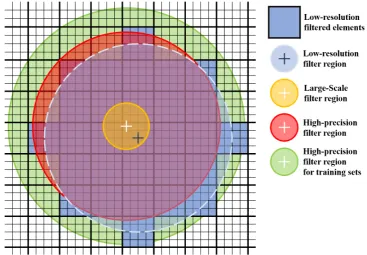
As mentioned in the section of density-based topology optimization methods, there is a sensitivity filter in topology optimization defined by the filter radius rmin. For ease of explanation, this article uses the element number as the unit of filter radius, and defines the actual radius length as the true radius. The filter radius links the mesh size to the model size. Both large-scale and high-precision are closely related to the increase in resolution (i.e. high-resolution), but the model size, element size and filter radius vary differently. Compared with the low-resolution model, the large-scale model only increases the model size, and the element size and filter radius are maintained. The high-precision model size is unchanged and the element size becomes smaller, and the filter radius is increased.
Fig. 3 Filter region and filtered elements of different high-resolution transformations.
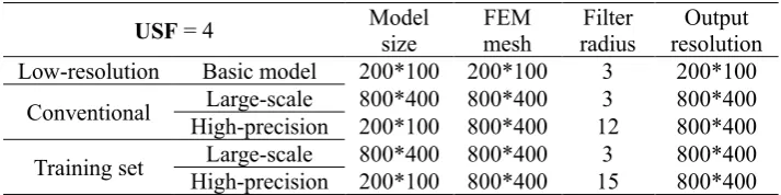
USF = 4 Model size FEM mesh radius Filter resolution Output Low-resolution Basic model 200*100 200*100 3 200*100
Conventional High-precision 200*100 800*400 Large-scale 800*400 800*400 12 3 800*400 800*400
Training set High-precision 200*100 800*400 Large-scale 800*400 800*400 15 3 800*400 800*400
For the specific case, Table 1 shows a base model with a mesh of 200*100 and a filter radius of 3 (the number of elements is used as the unit of the filter radius). When the USF is used to increase the resolution with a value of 4, the parameter changes of large-scale and high-precision are displayed. In Fig. 3, the blue circular area and the blue large element represent the filter region and the filtered element of the low-resolution base model, respectively. We can observe from the Table 1 that in the conventional method, when dealing with large-scale models, the model size and finite element mesh are increased to 800*400, and the filter radius is kept at 3, corresponding to the yellow area in Fig. 3. For high-precision models, the model size remains at 200*100, while the finite element mesh is increased to 800*400 and the filter radius is increased to 12, corresponding to the red area in the Fig. 3.
We have found that the high-precision filter region of the conventional method in Fig. 3 does not include all of the filtered elements in low-resolution. SRCNN is a method that relies on data. Therefore, in order to ensure that the training set of the neural network can contain all the necessary data information, we use the following filter radius conversion formula for the SRCNN training set.
(
)
(
)
min min
min min
1 1
1 1
H L
L H
r r USF
r r USF
= + × −
= + −
(10)
where rminH and rminL are the filter radius of high and low-resolution mesh, and USF is the upscaling factor. As can be seen from Table 1, the training set using the filter radius conversion formula has a high-precision filter radius of 15, corresponding to the green area in Fig 3. In this way, the filter area contains all the necessary data information.
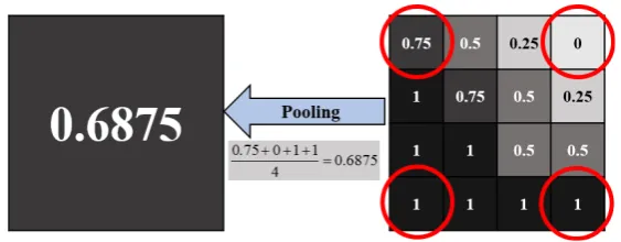
4.2 Pooling
Fig. 4 The pooling strategy with corner mean sampling 4.3 Numerical implementation
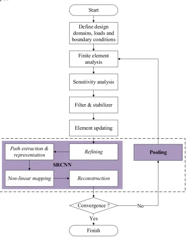
Now a high-resolution topology optimization method (HRTO) is established by implementing SRCNN and Pooling strategies as shown in Fig.5. HRTO separates the output configuration mesh from finite element mesh through SRCNN, and Pooling connects them. Therefore, the high-resolution information obtained by SRCNN can still have an impact on finite element analysis while maintaining efficient computation. In HRTO process, the stabilizer and convergence criteria used in the BESO method (Huang and Xie 2007) were introduced in order to improve convergence. If the filter scheme (Sigmund 2001) can smooth the sensitivity in space, then the stabilizer makes the sensitivity smooth in time.
The procedure of the present high-resolution topology optimization method is given as follows:
(1)Define the FEA mesh of the design domain and its load and boundary conditions, and then assign the initial design variable value (0 or 1) to each element.
(2)Analyze the design with FEA method.
(3)Calculated the sensitivity of individual elements with the data obtained from FEA.
(4)Use a filter (Sigmund 2001) to smooth the sensitivity spatially and the stabilizer
(
1)
ˆi = i+ i− 2
α α α (Huang and Xie 2007) to smooth the sensitivity temporally.
(5)Update design variables with OC method.
(6)Increase the resolution of design variables with SRCNN.
(7)Determine whether the optimization design satisfies the convergence condition
(
1 1)
1
1 1
N
k i k N i i
N k i i
C C
error
C τ
− + − − + =
− + =
−
=
∑
≤∑
. If not, pooling will be executed to reduce the designresolution.
(8)Repeat steps 2-7 until the convergence condition is satisfied. 4.4The combination treatment of 3D models
in each of three directions, an element of 1*1*1 is gradually shifted to 16*16*16 elements. The location of SRCNN in the topology optimization and the different processing methods of the 2D and 3D models have been determined. The next section will show how it works in some numerical examples.
SRCNN
Start
Finite element analysis
Finish Element updating Sensitivity analysis
Filter & stabilizer
No Define design
domains, loads and boundary conditions
Refining
Convergence ?
Yes
Pooling
Reconstruction Non-linear mapping
Path extraction & representation
Fig. 5 High-Resolution Topology Optimization Method. The part inside the dotted box is the high-resolution process introduced by HRTO method in traditional topology optimization.
5 Numerical examples
This section uses the HRTO method to solve topology optimization problem. We use the efficient topology optimization code, released by Andreassen et al. (2011), as the base program. All examples are operated on the same computer, and their hardware includes an Inter(R) Xeon(R) CPU E5-2689 v4 @ 3.10Ghz and 256g RAM. None of them uses GPU parallelism.
5.1 2D numerical examples
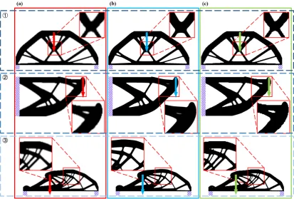
Fig. 7 shows several results of numerical examples with the network we trained using the topology optimization dedicated training set. The case ① is a MBB beam model with the
low-resolution mesh of 240 100× . And its target volume and filter radius are 0.4 and 15
respectively. Its load is applied to a random location on the upper part of design domain. For case
②, it is a cantilever beam model with the low-resolution mesh of 240 120× . And the position of
the load is at a random point on the right side of the design domain. The target volume and filter radius are 0.4 and 15 respectively. Another MBB beam model as case ③ has the
low-resolution mesh of 260 120× , the target volume of 0.3 and the filter radius of 11. A random point to the left of the design domain is loaded. The high-resolution USF of the above models are 4. The optimization parameters of these several examples and the loaded nodes numbers are random values. These examples were isolated from the training set, so the possibility of data leakage was eliminated.
Fig. 7 The comparison of optimization results of three random cases ①, ②, and③. (a) is the low-resolution optimization result, and (b) and (c) are high-resolution optimization results using the
conventional method and the HRTO method, respectively.
case ①, which is in line with our research expectations. And its ability to identify and correct
gray elements as the case ② is an unexpected performance. The case ③ shows the mesh
independent characteristics of the HRTO method, and its design retains characteristics of the low-resolution model, which ensures the reliability of the results.
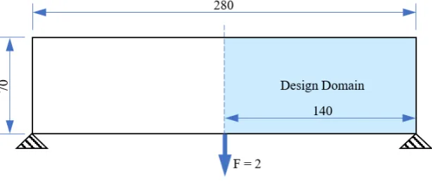
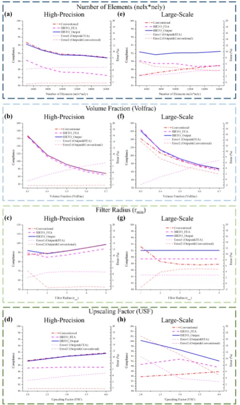
In order to investigate the influence of each optimization parameter on HRTO efficiency, we choose an MBB beam as the base model, half of which is used as an optimization model in Fig. 8. Its E=1, load F =2, and its optimization parameters include a base resolution of 140*70, a target volume of 0.5, a filter radius of 3, and a upscaling factor of 4. Therefore, the output resolution will reach 560*280. Table 2 lists alternative optimization parameters for parametric analysis.
Fig. 8 MBB beam basic model
Table 2 Alternative optimization parameters Basic
resolution volume Target radius Filter Upscaling factor
100*50 0.3 1 2
120*60 0.4 2 3
Basic model 140*70 0.5 3 4
160*80 0.6 4
180*90 0.7 5
the objective function decreases with increasing individual optimization parameters Fig. 9(e), (f), and (h) (except for the filter plate radius rmin in Fig. 9(g)), but it is only reduced to around 5%. It can also be observed in Fig. 9(a)-(h) that the high-resolution design sacrifices about 5% performance compared to the low-resolution design not processed by SRCNN.
Fig. 9 The influence of each optimization parameter of 2D designs on objective
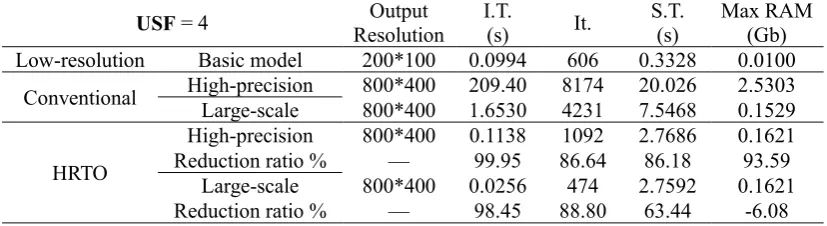
compliance calculated by FEA. According to the test of Fig. 9, the output compliance of the HRTO method is about 5% higher than that of FEA. In Fig. 10, the convergence of the HRTO method is significantly better than the conventional method. And Table 3 shows several specific data on the convergence history of Figure 10. As can be seen further from Table 3, HRTO is a very efficient method. For high-precision models, because of the lower resolution of FEM mesh and the smaller filter radius, HRTO only needs to add a small amount of memory required for neural network operations, which can reduce the Initial Time (I.T.) by 99.95% and the Step Time (S.T.) by 86.18%. In addition, SRCNN includes filter characteristics, so the iteration number (It.) is also reduced, which is about 86.64%. For large-scale models, the computational efficiency is also improved. For the above three data, the Initial Time (I.T.), the Step Time (S.T.), and the iteration number (It.) were reduced by 98.45%, 88.80% and 63.44%, respectively. These improved performances combine to save users a lot of time and computing costs. The conventional method requires a large amount of running memory in the high-precision case, and HRTO method requires less. By comparing with the large-scale case of the two methods, it can be found that the conventional method requires a large memory space to calculate the filter of high-precision case, and the peak of memory of HRTO occur in neural network computation.
Fig. 10 The MBB beam convergence history of the conventional method and the HRTO method. The compliance curves associated with the HRTO method are calculated from the FEA mesh rather than output designs. After testing, the compliance of HRTO output designs is about 5% larger than the value
in this figure.
Table 3 The MBB beam efficiency of the conventional methods and the HRTO methods USF = 4 Resolution Output I.T. (s) It. S.T. (s) Max RAM (Gb) Low-resolution Basic model 200*100 0.0994 606 0.3328 0.0100
Conventional High-precision Large-scale 800*400 209.40 800*400 1.6530 8174 4231 20.026 7.5468 2.5303 0.1529
HRTO
High-precision 800*400 0.1138 1092 2.7686 0.1621 Reduction ratio % — 99.95 86.64 86.18 93.59
Large-scale 800*400 0.0256 474 2.7592 0.1621 Reduction ratio % — 98.45 88.80 63.44 -6.08
to the MBB beam of Fig. 8. In addition to the change in resolution, the unlisted optimization parameters include a target volume equal to 0.5, a filter radius of 3, and an upscaling factor of 4 are constants. The data in the table shows that HRTO has a stable ability to accelerate high-precision models, and the acceleration capability of large-scale models increases with resolution.
Table 4 The efficiencies of the HRTO method at different resolutions Basic
Resolution Resolution Output
Conventional HRTO
I.T.
(s) S.T. (s) I.T. (s) Reduction ratio % S.T. (s) Reduction ratio % High-precision
100*50 400*200 15.19 4.591 0.023 99.85 0.660 85.63 120*60 480*240 24.89 7.166 0.039 99.84 0.905 87.37 140*70 560*280 37.55 7.068 0.054 99.86 1.254 82.25 160*80 640*320 58.13 9.790 0.073 99.88 1.719 82.44 180*90 720*360 121.0 14.14 0.088 99.93 2.115 85.04 200*100 800*400 209.4 20.03 0.114 99.95 2.769 86.18
Large-scale
100*50 400*200 0.539 1.710 0.006 98.85 0.695 59.37 120*60 480*240 0.731 2.607 0.007 99.00 0.899 65.51 140*70 560*280 0.746 2.794 0.010 98.66 1.230 56.00 160*80 640*320 1.015 3.935 0.014 98.66 1.631 58.54 180*90 720*360 1.342 5.089 0.021 98.41 2.015 60.40 200*100 800*400 1.653 7.547 0.026 98.45 2.759 63.44
5.2 3D numerical examples
Fig. 11 shows the computing power of the HRTO method in 3D models. The base resolution of this cantilever beam is 100*20*10, volume fraction vol=0.35, filter radius rmin=2, upscaling factor USF=4. With the help of the combination treatment of 3D models, the output resolution was increased to 16 times in all three dimensions, i.e. 1600*320*160, and the output designs included a total of 81,920,000 elements. This example doesn’t require strong hardware support, and it can be performed on a typical computer. This computer includes Intel(R) Core (TM) i5-7500 CPU @ 3.40Ghz and 4Gb RAM. It requires only 0.57s for initialization and 651.41s for a single step. Under the same hardware conditions, conventional methods are difficult to run, so the design of conventional method can’t be shown here. Again, the high computational efficiency of the proposed method is highlighted.
6
Conclusions and Remarks
This paper proposes an efficient high-resolution topology optimization method using SRCNN. In this framework, the two strategies are developed, i.e. the pooling strategy for mesh balance and a combined treatment method using 2D SRCNN. This method allows 3D HRTO to eliminate significant computational costs. From a comprehensive comparison, the following conclusions can be drawn:
(1)In terms of resolution, the data used in this paper increases the resolution of the 2D model from 200*100 to 800*400, and the resolution of the 3D model from 100*20*10 to 1600*320*160. By flexibly combining SRCNN and Pooling modules, the HRTO method can make the design reach any resolution.
(2)Regarding to efficiency, HRTO is much more efficient than traditional algorithms. In a high-precision design, the iteration number is reduced from 8174 to 1092, and the step time is reduced from 20.026 seconds to 2.7686 seconds. After further testing, the acceleration effect becomes more and more apparent as the number of meshes in the design domain increases.
(3)From the perspective of versatility, HRTO benefits from the wide application scenarios of SRCNN, and it is more versatile than other topology optimization methods using neural networks. HRTO can be selected for any design domain, any number of meshes, arbitrary boundary conditions and loads. However, it should be noted that the number of FEA meshes should reach the mesh independent threshold to ensure reasonable design.
Acknowledgements
Reference
Aage N, Andreassen E, Lazarov BS, Sigmund O (2017) Giga-voxel computational morphogenesis for structural design. Nature 550:84–86. doi: 10.1038/nature23911
Alexandersen J, Sigmund O, Aage N (2016) Large scale three-dimensional topology optimisation of heat sinks cooled by natural convection. Int J Heat Mass Transf 100:876–891. doi:
10.1016/j.ijheatmasstransfer.2016.05.013
Andreassen E, Clausen A, Schevenels M, et al (2011) Efficient topology optimization in MATLAB using 88 lines of code. Struct Multidiscip Optim 43:1–16. doi: 10.1007/s00158-010-0594-7 Banga S, Gehani H, Bhilare S, et al (2018) 3D Topology Optimization using Convolutional Neural
Networks. arXiv preprint arXiv: 1808.07440v1
Bendsøe MP (1989) Optimal shape design as a material distribution problem. Struct Optim 1:193–202. doi: 10.1007/BF01650949
Bendsøe MP (2009) Topology optimization. Springer ISBN: 0387747583
Bendsøe MP, Kikuchi N (1988) Generating optimal topologies in structural design using a homogenization method. Comput Methods Appl Mech Eng 71:197–224. doi: 10.1016/0045-7825(88)90086-2
Challis VJ, Roberts AP, Grotowski JF (2014) High resolution topology optimization using graphics processing units (GPUs). Struct Multidiscip Optim 49:315–325. doi: 10.1007/s00158-013-0980-z Chin TW, Kennedy GJ (2016) Large-scale compliance-minimization and buckling topology
optimization of the undeformed common research model wing. 57th AIAA/ASCE/AHS/ASC Struct Struct Dyn Mater Conf. doi: 10.2514/6.2016-0939
Chin TW, Leader MK, Kennedy GJ (2019) A scalable framework for large-scale 3D multimaterial topology optimization with octree-based mesh adaptation. Adv Eng Softw 135:102682. doi: 10.1016/j.advengsoft.2019.05.004
Christiansen AN, Bærentzen JA, Nobel-Jørgensen M, et al (2015) Combined shape and topology optimization of 3D structures. Comput Graph 46:25–35. doi: 10.1016/j.cag.2014.09.021
Dong C, Loy CC, He K, Tang X (2016) Image Super-Resolution Using Deep Convolutional Networks. IEEE Trans Pattern Anal Mach Intell 38:295–307. doi: 10.1109/TPAMI.2015.2439281
Groen JP, Langelaar M, Sigmund O, Ruess M (2017) Higher-order multi-resolution topology optimization using the finite cell method. Int J Numer Methods Eng 110:903–920. doi: 10.1002/nme.5432
Groen JP, Sigmund O (2018) Homogenization-based topology optimization for high-resolution manufacturable microstructures. Int J Numer Methods Eng 113:1148–1163. doi:
10.1002/nme.5575
Guo X, Zhang W, Zhong W (2014) Doing topology optimization explicitly and geometrically: A new moving morphable components based framework. Front Appl Mech 81:31–32. doi:
10.1115/1.4027609
Gupta DK, van Keulen F, Langelaar M (2018) Design and analysis adaptivity in multi-resolution topology optimization. arXiv preprint arXiv:1811.09821
evolutionary structural optimization method. Finite Elem Anal Des 43:1039–1049. doi: 10.1016/j.finel.2007.06.006
Kim YY, Yoon GH (2000) Multi-resolution multi-scale topology optimization - A new paradigm. Int J Solids Struct 37:5529–5559. doi: 10.1016/S0020-7683(99)00251-6
Leader MK, Chin TW, Kennedy GJ (2019) High-Resolution Topology Optimization with Stress and Natural Frequency Constraints. AIAA J 57:3562–3578. doi: 10.2514/1.j057777
Lei X, Liu C, Du Z, et al (2019) Machine learning-driven real-time topology optimization under moving morphable component-based framework. J Appl Mech Trans ASME 86:1–9. doi: 10.1115/1.4041319
Li B, Huang C, Li X, et al (2019) Non-iterative structural topology optimization using deep learning. CAD Comput Aided Des 115:172–180. doi: 10.1016/j.cad.2019.05.038
Liao Z, Zhang Y, Wang Y, Li W (2019) A triple acceleration method for topology optimization. Struct Multidiscip Optim 60:727–744. doi: 10.1007/s00158-019-02234-6
Lieu QX, Lee J (2017) Multiresolution topology optimization using isogeometric analysis. Int J Numer Methods Eng 112:2025–2047. doi: 10.1002/nme.5593
Liu J, Ou H, He J, Wen G (2019) Topological Design of a Lightweight Sandwich Aircraft Spoiler. Materials (Basel) 12:3225. doi: 10.3390/ma12193225
Nguyen-Xuan H (2017) A polytree-based adaptive polygonal finite element method for topology optimization. Int J Numer Methods Eng 110:972–1000. doi: 10.1002/nme.5448
Nguyen TH, Paulino GH, Song J, Le CH (2010) A computational paradigm for multiresolution topology optimization (MTOP). Struct Multidiscip Optim 41:525–539. doi:
10.1007/s00158-009-0443-8
Querin OM, Steven GP, Xie YM (1998) Evolutionary structural optimisation (ESO) using a bidirectional algorithm. Eng Comput (Swansea, Wales) 15:1031–1048. doi:
10.1108/02644409810244129
Rozvany GIN (2009) A critical review of established methods of structural topology optimization. Struct Multidiscip Optim 37:217–237. doi: 10.1007/s00158-007-0217-0
Rozvany GIN, Zhou M, Birker T (1992) Generalized shape optimization without homogenization. Struct Optim 4:250–252. doi: 10.1007/bf01742754
Sigmund O (2001) A 99 line topology optimization code written in matlab. Struct Multidiscip Optim 21:120–127. doi: 10.1007/s001580050176
Sosnovik I, Oseledets I (2017) Neural networks for topology optimization. Russ J Numer Anal Math Model 34:215–223. doi: 10.1515/rnam-2019-0018
Stainko R (2006) An adaptive multilevel approach to the minimal compliance problem in topology optimization. Commun Numer Methods Eng 22:109–118. doi: 10.1002/cnm.800
Sun Y (2006) Machine Learning. In: https://baike.baidu.com/item/%E6%9C%BA%E5%99%A8%E5% AD%A6%E4%B9%A0/217599
Suresh K (2013) Generating 3D Topologies with Multiple Constraints on the GPU. 10th World Congr Struct Multidiscip Optim pp 1–9
using a novel topology optimization method. Med Biol Eng Comput 54:1123–1135. doi: 10.1007/s11517-015-1418-0
Wang H, Liu J, Wen G (2019a) An efficient evolutionary structural optimization method with smooth edges based on the game of building blocks. Eng Optim doi: 10.1080/0305215X.2018.1562550 Wang H, Liu J, Wen G (2019b) Achieving large-scale or high-resolution topology optimization based
on Modified BESO and XEFM. arXiv preprint arXiv:1908.07157
Wang MY, Wang X, Guo D (2003) A level set method for structural topology optimization. Comput Methods Appl Mech Eng 192:227–246. doi: 10.1016/S0045-7825(02)00559-5
Wei P, Li Z, Li X, Wang MY (2018) An 88-line MATLAB code for the parameterized level set method based topology optimization using radial basis functions. Struct Multidiscip Optim 58:831–849. doi: 10.1007/s00158-018-1904-8
Wu Z, Xia L, Wang S, Shi T (2019) Topology optimization of hierarchical lattice structures with substructuring. Comput Methods Appl Mech Eng 345:602–617. doi: 10.1016/j.cma.2018.11.003 Xie YM, Steven GP (1993) A simple evolutionary procedure for structural optimization. Comput Struct
49:885–896. doi: 10.1016/0045-7949(93)90035-C
Xu M, Xia L, Wang S, et al (2019) An isogeometric approach to topology optimization of spatially graded hierarchical structures. Compos Struct 225:111171. doi:
10.1016/j.compstruct.2019.111171
Zhang W, Chen J, Zhu X, et al (2017) Explicit three dimensional topology optimization via Moving Morphable Void (MMV) approach. Comput Methods Appl Mech Eng 322:590–614. doi: 10.1016/j.cma.2017.05.002
Zhang Y, Chen A, Peng B, et al (2019) A deep Convolutional Neural Network for topology optimization with strong generalization ability. arXiv preprint arXiv:1901.07761
Zhu B, Skouras M, Chen D, Matusik W (2017) Two-scale topology optimization with microstructures. ACM Trans Graph 36:. doi: 10.1145/3095815