Reliable Categorical Clustering

(1)

Reliable Categorical Clustering

Sardhendu Mishra

Dell IT

Abstract

—Clustering in data mining is necessary for finding patterns and distribution of the dataset. Traditional clustering algorithms that uses distance based approach does not produce good clusters with categorical datasets. Traditional clustering algorithms like k-modes and k-means are sensitive to outliers and require the number of clusters to be specified beforehand. The clustering in traditional approach highly depends on the selection of initial centroids or initial modes. Since the centroid and the modes for these algorithms are chosen randomly, they cannot be relied upon to generate robust clusters. In this paper we present an approach to cluster categorical dataset using a similarity measure. Then we present a novel way of selecting the initial centroids that takes care of the outliers. By leveraging the similarity measure and the selection of initial centroids we employ the concepts of clustering with canopy on top the traditional k-means algorithm to cluster the dataset.

Keywords: Data mining, clustering algorithm, Categorical data, k-means, k-modes, ROCK, Spectral Clustering

I. INTRODUCTION

Clustering in data mining has been of paramount importance for various tasks like discovering patterns in the dataset, understanding the structure of the dataset and many others. Clustering is a technique to group data with similar characteristics. Today much of the data like product data, customer purchase data, marketing data, social media data and etc. that contains enormous information of a domain are in the form of categorical datasets or text datasets. Traditional clustering algorithm like k-means is productive with numerical data in which each cluster has a mean and the algorithm minimizes the sum of squared distance between each data point to its closest center [1]. Since k-means algorithm works by finding the mean that requires numerical data type, the algorithm cannot be implemented on categorical dataset where the data is nominal. Clustering algorithms designed to cluster categorical dataset like k-modes- clusters the data points based on the selection of initial modes. The clustering in k-modes highly depends on the selection of initial modes and is also sensitive to outliers [2]. Clustering algorithms based on the computation of pairwise similarity of the datasets have recently

gained a lot of importance because of their simplicity and effectiveness in finding good clusters [4]. However, it faces a problem while applying to huge datasets: (1) it requires to compute and store the huge similarity matrix. This problem can be addressed by sparsifying the similarity matrix and using multiple machines for parallel computing [6] & [7]. The similarity matrix depicts a space in higher dimension where the intra-cluster distance between the data points is believed to be higher and inter-cluster distance between the data points is believed to be lower. A simple algorithm uses basic k-means to cluster the transformed dataset. In this paper we define an approach of clustering categorical datasets by constructing the sparse similarity matrix using Jaccard similarity measure. We then use sparse Eigen solvers (ARPACK) to quickly obtain the first

d

eigen vectors and reduce the dimension of the similarity matrix. By leveraging the information in the similarity matrix we then present an approach of selecting the initial centroids and perform clustering using k-means. We also employ general concept of clustering with canopy on top of the k-means algorithm to reduce the overall run time [8].

We evaluate the performance of the algorithm with few public datasets available in the UCI repository and compare them to traditional K-modes clustering approach [6].

The rest of the paper is organized as follows. Section 2 describes few related algorithms. Section 3 describes the computation of similarity matrix using a similarity model and dimensional reduction using fast Eigen solvers. Section 4 describes an approach of finding the initial centroids based on the similarity matrix. Section 5 describes the k-means clustering algorithm coupled with the clustering with canopy approach. Section 6 presents the flowchart of the entire process. In section 7, we compare the results of our approach with a traditional categorical clustering approach.

II. RELATED WORK

Many clustering algorithm have been proposed in the past to deal with different types of datasets like Numerical datasets, Text datasets, categorical datasets, mixed numerical and nominal datasets and many others. However, no one algorithm can be relied upon to produce best clusters for all the possible problems.

(2)

in which the dataset is clustered into clusters by finding the centers that minimizes the sum of squared distance of each data point to its closest center.

K-modes: The k-modes clustering algorithm is an extension of the k-means clustering algorithm in which it replaces the means with modes. The k-modes algorithm tends to minimize the dissimilarity between the objects and their modes. A mode is a row vector where each element corresponds to a categorical value pertaining to an attribute. The algorithm takes the number of cluster as an input, randomly selects the initial modes and groups all the objects to their nearest modes. It is an iterative process where the modes are replaced with the most frequent attribute value of a group and the iteration persists until the modes in two successive iteration remains same.

ROCK: ROCK is an agglomerative hierarchical clustering algorithm that uses the concept of links to group objects into a cluster and merge clusters. The link between a pair of records is defined as the number of common neighbors and the objects are said to be neighbors if there similarity exceeds a certain threshold value. Objects belonging to a cluster would generally have large number of common neighbors and thus have more links.

Spectral clustering: Spectral clustering clusters the dataset by constructing a similarity matrix where each element in the matrix is the pairwise similarity between two rows. The data points are then projected into a new subspace created by the top eigen vectors and a distance based clustering approach like k-means is used to cluster the data points in the subspace spanned by the first eigen vectors.

III. PAIR-WISE SIMILARITY

For a given dataset the similarity between any two rows is defined by Jaccard similarity coefficient.

For any pair of rows and the similarity function

is a function where

thus making the similarity matrix symmetric. The similarity matrix is a dense matrix. For large datasets

therefore we modify the matrix into a sparse matrix by zeroing out the similarity value where the similarity coefficient is less than the provided threshold .

.

The sparse similarity matrix consumes very less space when compared to the similarity matrix , where t denotes the number of non-zero elements in the similarity matrix [9].

Finding first

d

Eigen vectors: After obtaining the sparse matrix we use sparse eigen solvers to find the first d eigen vectors. We use the ARPACK package that quickly obtains first

d

Eigen vectors of the similarity matrix

S

. Then we take the dot product of the similarity matrix

S

m m× and the first

d

eigen vectors and transform the similarity matrix into a lower dimensional vector space

(

S

m×d

)

, where m denotes the number of rows and

d

denotes the dimensions. This reduced similarity matrix

(

S

m×d

)

is then used for clustering data points.

IV. CHOOSING CENTROIDS

Choices of initial centroids play a crucial role in finding clusters in the k-means algorithm. For random initialization of centroids there lies a high chance for the algorithm to get stuck in the local minima, which results in bad clustering. Therefore, k-means algorithm is required to be run multiple times with random initialization of centroids. Re-running the algorithm multiple times for a large dataset could be costly. Moreover, the k-means algorithm is sensitive to outliers and requires the number of clusters to be specified beforehand.

In this section we provide and evaluate a simple approach to choose the initial centroids, which is based on the computation of pairwise similarity.

Based on the specified threshold value we create overlapping groups with each group containing the data points that are similar to each other. Points within a group are tightly coupled. Our approach is to consider any one element of each group as the centroid of that group, provided the point is not in the overlapping region.

k

( )

k

1 2

{

,

,...

_m

}

X

=

X X

X

( _i, _j) i j

i j

X X S X X

X X

∩ =

∪

{

1, 2, 3 .

}

&

{

1, 2, 3,

}

for i= …m j= …m

i

X

_j

(

_i

,

_j

)

S X X

(

_i

,

_j

)

=

S X

(

_j

,

X

_i

)

m m

S

∈

R

×

m m

S

×

S

3

t

S

×

( )

θ

(

_i

,

_j

) 0

(

_i

,

_j

)

S X X

=

if S X X

<

θ

3

t

S

×

m m

S

×

( )

θ

(3)

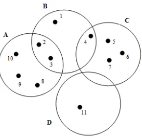
Fig1.1: Overlapping group of data points

In the given figure 1.1 we have four groups. For a given threshold value the similarity for each data point can be written as:

Data point 1 is similar to data points 1, 2, 3 and 4 Data point 2 is similar to data points 1, 2, 3, 4, 8, 9 and 10 Data point 3 is similar to data points 1, 2, 3, 4, 8, 9 and 10 Data point 4 is similar to data points 1, 2, 3, 4, 5, 6 and 7 Data point 5 is similar to data points 4, 5, 6 and 7 Data point 6 is similar to data points 4, 5, 6 and 7 Data point 7 is similar to data points 4, 5, 6 and 7 Data point 8 is similar to data points 2, 3, 8, 9 and 10 Data point 9 is similar to data points 2, 3, 8, 9 and 10 Data point 10 is similar to data points 2, 3, 8, 9 and10 Data point 11 is similar to data points 11

Data points that are distant from other data points are considered as outliers. In the figure 1.1 all the data points except point 11 are tightly or loosely coupled with one another. Because data point 11 has no connection to any of the other data points, it can be considered as an outlier. The selection of centroids is based on two primary concepts: (1) choosing points in the order of their occurrence and (2) excluding the data point that belong to the same group of the previously chosen centroids.

In figure (1.1), data point 11 is chosen as the first centroid because it has the least number of connections, data point 1 is chosen as the second centroid, data point 5 is chosen as the third centroid as data points 2, 3 and 4 are tightly coupled to data point 1 and data point 8 is chosen as the fourth centroid because data points 6 and 7 are tightly coupled with centroid 5. Running the k-means algorithm on the data points for the chosen centroids gives four clusters.

Cluster1: 11 Cluster2: 1

Cluster3: 4, 5, 6 and 7 Cluster4: 2, 3, 8, 9 and 10

Algorithm:

Initialization of Cluster Centroids

1. Create a dictionary (similarity_dict) with “keys” as data points id and “values” as a list of ids of similar data points. Order the dictionary by the count of ids in the “values”. For Example, for data points in fig 1.1 the similarity_dict will look like, { 11:[11], 1: [1,2,3,4], 5:[4,5,6,7], 6:[,4,5,6,7], 7:[4,5,6,7], 8:[2,3,8,9,10], 9:[2,3,8,9,10], 10:[2,3,8,9,10],

2:[1,2,3,4,8,9,10],

3:[1,2,3,4,8,9,10], 4:[1,2,3,4,5,6,7] }

2. Function find_centroid (similarity_dict): 3. centroid_ids=[]

4. excluded_ids=[]

6. for keys, values in similarity_dict: 7. If keys not in excluded_ids 8. centroid_ids.append(keys)

9. excluded_ids= excluded_ids+values 10. else:

11. continue 13. return centroid_ids

Table 1: Algorithm for Cluster centroid Initialization

The algorithm doesn’t require a cluster number to be specified, the number of clusters are decided implicitly by the algorithm based on the threshold value provided. Experiments performed on various public datasets shows that a threshold value within the range of 0.3 and 0.5 results in good clusters.

V. CLUSTERING WITH K-MEANS

K-means is one of the most widely used clustering algorithms for variety of tasks like preprocessing the dataset or finding patterns in the underlying data. K-means partitions the dataset by minimizing the sum of squared distance between the data point to its nearest cluster. The algorithm is an iterative process that operates by calculating the Euclidean distance between all the data points and chosen centroids.

For a given matrix , denotes the number of rows and denotes the number of dimensions of the reduced similarity matrix . For centroids the k-means is defined as:

For a very large dataset the computation of distance between all

the data points and the centroids can be computationally

( )

θ

m d

X

∈

R

×

m

d

ij

S

c

=

{ ,

c c

₁ ₂

,.... }

c

_k

2

1

k

j i

i X_j c_i

X

c

= ∈

−

∑ ∑

for j

1, 2,..

=

{

m

}

(4)

the group to which the centroid belongs [9]. Data points belonging to different groups are assumed to be far from each other. In figure 1.1, it is highly unlikely that data points 1 and 10 or data points 1 and 7 would fall under the same cluster. For a centroid in group (A) the distance of the centroid would only be computed for data points 2,3,8,9 and 10.

From the initial centroids selection as mentioned in section 4 we ensure that each group is assigned with a centroid, which is a data point in that group. So it is highly unlikely that the centroids belonging to a group would move entirely to another group, however, the centroid may move to the overlapping region at times when data points in the overlapping region are more in number than the data points in non-overlapping region of a particular group. With the above case the algorithm still ensures that all the data points are covered and clustered.

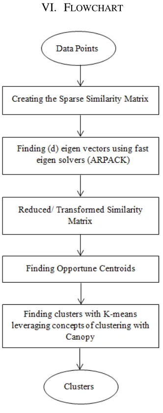
VI. FLOWCHART

Fig 1.2 Flowchart of the entire process

The algorithm was run for few real life datasets like Congressional votes, Mushroom dataset and Soybean dataset present in the UCI Machine learning repository and was compared to traditional algorithms like k-modes. The algorithm showed comparatively good results when the threshold values were set more than 0.3.

Congressional Votes dataset: The dataset is taken from UCI repository. It contains 435 records with each records corresponding to one congress man’s vote and 16 attributes with few entries missing. Each row is labeled with a class Democrat or Republican with 168 records labeled Republican and 267 records labeled Democrat.

The algorithm was run for the dataset with a threshold value . The number of clusters produced was 13

K-modes for 10 runs with random initialization of centers

Clust er NO

No. of Democ rats

No. of Republi c

Cluster NO

No. of Democ rat

No. of Republi c

1 6 84 8 34 0

2 4 13 9 18 0

3 21 0 10 8 1

4 0 18 11 59 0

5 2 2 12 12 0

6 50 0 13 2 49

7 51 0

Reliable Categorical Clustering

Clust er NO

No. of Democ rats

No. of Republi c

Cluster NO

No. of Democ rat

No. of Republi c

1 1 0 8 0 132

2 132 0 9 1 0

3 19 1 10 0 1

0.3 θ

=

(5)

4 12 4 11 1 22

5 1 4 12 67 2

6 18 1 13 15 0

7 0 1

Table 2: Clustering results for Congressional Votes dataset

Table 2 shows the result of running the K-modes and the proposed categorical clustering algorithm for Congressional Votes. The clustering with k-modes was run with 10 random initialization of centroids and the best among them that minimized the sum of squared error was chosen to be the centroids. It can be inferred from the Table 2 that clustering quality of the proposed algorithm is better than that of k-modes taking two objectives in mind. (1) It takes care of the outliers: Cluster No. 1,5,7,9 and 10 can be considered as outliers as they are present in small group, and (2) It produces robust and pure clusters, for example, cluster no. 2 and cluster no. 8 with the largest number of data points have all the data point belonging to one particular class.

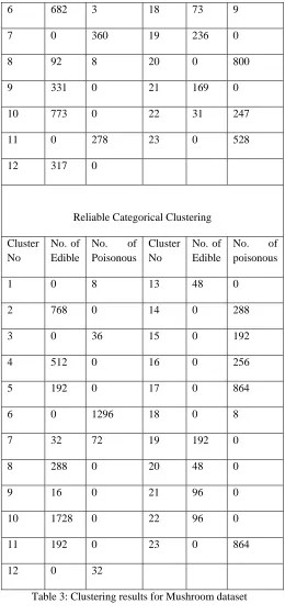
Mushroom Dataset: The dataset is taken from UCI repository. It contains 8124 records and 22 attributes with few missing entries. Each record is labeled either poisonous (p) or edible (e) with 4208 records labeled edible and 3916 records labeled poisonous.

The algorithm was run for the dataset with a threshold value = 0.45. The number of clusters produced was 23.

Cluster No

No. of Edible

No. of Poisonous

Cluster No

No. of Edible

No. of poisonous

1 438 24 13 43 194

2 0 216 14 24 240

3 0 571 15 0 124

4 362 0 16 291 0

5 346 0 17 0 314

6 682 3 18 73 9

7 0 360 19 236 0

8 92 8 20 0 800

9 331 0 21 169 0

10 773 0 22 31 247

11 0 278 23 0 528

12 317 0

Cluster No

No. of Edible

No. of Poisonous

Cluster No

No. of Edible

No. of poisonous

1 0 8 13 48 0

2 768 0 14 0 288

3 0 36 15 0 192

4 512 0 16 0 256

5 192 0 17 0 864

6 0 1296 18 0 8

7 32 72 19 192 0

8 288 0 20 48 0

9 16 0 21 96 0

10 1728 0 22 96 0

11 192 0 23 0 864

12 0 32

Table 3: Clustering results for Mushroom dataset

Table 3 shows the result of running the k-modes and the proposed categorical clustering algorithm for Mushroom dataset. The clustering with k-modes was run with 10 random initialization of centroids and the best among them that minimized the sum of squared error was chosen to be the centroids. It is obvious from the Table 3 that the proposed approach of Categorical clustering produces good cluster as all the clusters except one (Cluster No- 7) are pure clusters i.e. they are either Edible or poisonous whereas clustering using

θ

(6)

highly depends on the centroids chosen and since the centroids are chosen randomly the cluster may differ for every run and therefore cannot be relied upon. In the new approach presented the clusters would remain the same for every run. Also the variance in the cluster sizes in the presented new approach is very large (the cluster size varies from 8 to 1728) which validates the fact that the clusters are robust.

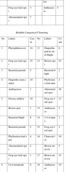
Soybean dataset: The soybean dataset is taken from UCI repository. It contains 307 rows and 35 attributes with few missing entries. Each record is labeled with one of the 19 classes.

The algorithm was run for the dataset with a threshold value = 0.45. The number of clusters produced was 21.

No Labels Co

unt

No Labels Cou nt

1 Bacterial-pustule 1 9 Anthracno se

14

Phyllosticla-leaf-s pot

2 Diaporthe

-pod-&-st em-blight

2

Alternarialeag-sp ot

14 10 Powdery-mildew

10

Frog-eye-leaf-spo t

2 11 Brown-ste m-rot

1

2 Cyst-nematode 6 Brown-sp

ot

5

2-4-d-injury=1 1 Bacterial-pustule

1

Herbicide-injury 4 Phyllostict a-leaf-spot

2

3 Brown-spot 3 12 Rhizocton ia-root-rot

10

Bacterial-blight 2 Phytophth ora-rot

16

Phyllosticta-leaf-s pot

1

Alternarialeaf-spo t

4 Brown-sp

ot

3

Frog-eye-leaf-spo t

7 Bacterial-blight

1

4 Brown-stem-rot 1 Alternaria leaf-spot

7

Purple-seed-stain 2 Frog-eye-l eaf-spot

1

8

5 Charcoal-rot 10 15 Frog-eye-l eaf-spot

10

Brown-stem-rot 2 16 Frog-eye-l eaf-spot

17

Purple-seed-stain 1 Purple-see d-stain

1

6 Downy-mildew 10 17 Brown-sp ot

13

7 Brown-spot 14 18 Bacterial-blight

6

bacterial-blight 1 Bacterial-pustule

5

Bacterial-pustule 1 19 Brown-ste m-rot

7

8 Brown-spot 2 Purple-see

d-stain 1

2 21 Diaporthe -pod-&-st em-blight

24

Bacterial-pustule 2 Phytophth ora-rot

4

Purple-seed-stain 2 21 Diaporthe -stem-can

10

θ

(7)

ker

Frog-eye-leaf-spo t

3 Anthracno

se

5

7

No Labels Cou

nt

No Labels Co unt

1 Phytophthora-rot 16 11 Diaporthe-pod-&-ste m-blight

6

2 Frog-eye-leaf-spo t

25 12 Brown-spo t

25

3 Bacterial-pustule 5 Bacterial-b light

2

4 Diaporthe-stem-c anker

10 Phyllostict a-leaf-spot

4

Anthracnose 1 Alternarial eaf-spot

38

5 Downy-mildew 10 Frog-eye-l eaf-spot

12

Brown-spot 1 13 Anthracno se

2

Bacterial-blight 8 14 2-4-d-injur y

1

Bacterial-pustule 5 15 Frog-eye-l eaf-spot

2

6 16 Charcoal-r ot

10

2 Brown-ste

m-rot

5

Frog-eye-leaf-spo t

15

6 Cyst-nematode 6 18 Anthracno se

10

7 Brown-spot 14 19 Rhizoctoni a-root-rot

10

8 Purple-seed-stain 10 20 Powdery-mildew

10

9 Anthracnose 7 21 Herbicide-i njury

4

10 Phytophthora-rot 24

Table 4: Clustering results for Soybean dataset Table 4 shows the result of running the k-modes and the proposed categorical clustering algorithm for Soybean dataset. The clustering with k-modes was run with 10 random initialization of centroids and the best among them that minimized the sum of squared error was chosen to be the centroids. From the Table 4 it can be inferred that clustering with k-modes does not produce good results as only 5 out of 21 clusters are pure clusters. On the other hand, clustering with the proposed approach produces 17 pure clusters.

VIII. CONCLUSION- FUTURE WORK

In this paper we present an approach to cluster categorical dataset using a pair-wise similarity measure. We then present a novel approach to find initial centroids that takes care of few of the limitations of the traditional approach. Leveraging the similarity measure we employ the concepts of clustering with canopy on top of k-means algorithm which reduces the run time of the k-means algorithm to a greater extent.

From the test results it can be inferred that the quality of clusters produced by the proposed approach is better when compared to 10 runs of traditional approach. The clusters are robust in there nature, the variance in the size of clusters generated by the approach is large when compared to the traditional approach. Outliers are handled well and misclassification of the data is low when compared to the traditional approach. For future work, we would like to apply the algorithm and standardize it for a distributed database system. By the use of distributed database systems, we believe, there will be a lot of performance gain when dealing with a very large dataset.

(8)

[1] K-means Clustering:

https://en.wikipedia.org/wiki/K-means_clustering

[2] Z.Huang, Extensions to the k-means algorithm for clustering large datasets with categorical values, Data Mining and Knowledge Discovery 2(1998) 283–304.

[3] R. Rastogi. S. Guha, K. Shim, Rock: a robust clustering algorithm for categorical attributes, Journal of Information Systems 25 (2000) 345–366.

[4] Ulrike von Luxburg: A Tutorial on Spectral Clustering, Statistics and Computing, 17(4):395-416, 2007

[5] UCI Machine Learning

Repository, 28TUhttps://archive.ics.uci.edu/ml/datasets.htmlU28T

[7] Wen-Yen Chen, Yangqui Song, Hongjie Bai, Chih-Jen Lin, Edward Y. Chang: Parallel Spectral Clustering in Distributed Systems

[8] Andrew McCallum, Kamal Nigam, Lyle H. Ungar: Efficient Clustering of High-Dimensional Data Sets with Application to Reference Matching,

http://www.kamalnigam.com/papers/canopy-kdd00.pdf

[9] Sparse matrices (scipy.sparse)

http://docs.scipy.org/doc/scipy/reference/sparse.html

[10] Gill David, Amir Averbuck: SpectralCAT: Categorical spectral clustering of numerical and nominal data, Pattern Recognition 45 (2012) 416–