Evolutionary methods for topology optimisation of continuum structures : static and dynamic problems

(1)

Evolutionary Methods for Topology

Optimisation of Continuum Structures:

Static and Dynamic Problems

by

Ms Xiaoying Yang, RE., M.E.

VICTORIA ^

UNIVfRSITY

m X 2 O I

-o

Thesis submitted in fulfilment of the requirement of

the degree of Doctor of Philosophy

to Victoria University of Technology

School of the Built Environment Victoria University of Technology

(2)

FTS THESIS

624.17713 YAN

30001007614284

Yang, Xiaoying

(3)

To my Sister, Xiaoyu

(4)

ACKNOWLEDGEMENTS

I wish to express my sincere gratitude to my supervisor. Prof, Mike Xie, Mike has been

offering unfailing support over the past years. He is always encouraging, patient and

responsive. Every student has been benefited from his prompt feedback when seeking

advice on a subject, a report or a paper, Mike always thinks of the welfare and career

development of his students and shares their concerns. He has provided me with great

career prospects and opportunities. His advice and support have been invaluable in my

securing a position with an engineering consultancy company. His understanding and

consideration are highly appreciated, especially when I have been occupied with the

thesis writing and a full-time job towards the end of the PhD study. I feel I am fortunate

to be one of his many postgraduate students, to have him as a mentor and friend, guiding

me through this important part of my life.

It is in the excellent School of Built Environment, Victoria University of Technology

that my postgraduate research has been carried out. The School has provided research

resources and facilities and a stimulating and positive study environment. My PhD study

has been sponsored by the Victoria University Postgraduate Research Scholarship,

which is gratefully acknowledged.

This thesis has benefited greatly from the Engineering Design Centre (EDC), of

University of Cambridge. Chapter 7 was the results of a six-month joint program in the

Centre under the supervision of Drs. P.J. Clarkson and G.T. Parks, who have led the

Design Optimisation Group (DOG). Dr. J.S. Liu, a group member and a major

collaborating researcher, has made invaluable effort and work on the joint program. The

Centre has sponsored me a conference in Swansea; And the group, especially Dr. G.T.

Parks, have helped me tremendously in preparing one journal paper. From the group and

its members, I have experienced the unique research culture and spirit of Cambridge.

Their kindness and assistance have made the stay fmitful and enjoyable.

I am grateful to Prof. G.P. Steven of University of Durham, U.K., the former Head of

Dept. of Aeronautical Engineering of University of Sydney, Australia. Thanks for his

(5)

University of Leeds, U.K., for his initial work on Bi-directional ESO (BESO), and his

advice and assistance. I have been inspired and encouraged by the researchers in

Melbourne and Sydney, especially by Dr. D. Manickarajah, Dr. Q. Li and Ms. W. Li.

Thanks also go to Prof. J.H. Rong who was a visiting research fellow on a ESO project.

His outstanding work and personal assistance are invaluable in the early stage of my

PhD study.

At the School of Built Environment, I wish to thank all the staff for their kindness and

encouragement, especially to Assoc. Prof. C. Perera, Dr. D. Tran, Assoc. Prof. O. Turan,

Ms. G. Geyer, Assoc. Profs. C. Bhuta, T. Graham and M. Sek. Special thanks are due to

Mr. T. Do who has helped greatly in the computer lab. Gratitude is extended to my

fellow students who have shared and experienced all the fmstrations and achievements

of being a research student. Thanks to David, Li, Anne and Quang, for their friendship.

Quang's computer excellence has been very helpful.

I wish to thank my fiance Qiang, who has always been by my side and put up with my

preoccupation with this thesis. Thanks for his understanding, caring love and

companionship.

Finally, it is a pleasure to acknowledge my family in China: my parents, my sister, my

brother-in-law and my little nephew. They are a source of constant love, understanding

and encouragement. I am deeply indebted to my sister, who has, in my absence, been

taking the family responsibility and making great sacrifice, and to whom, this thesis is

(6)

CERTIFICATE OF RESEARCH

This is to certify that except where specific reference to other investigation is made, the

work described in this thesis is the result of the candidate's own investigations.

Candidate

Supervisor

(7)

DECLARATION

This is to certify that neither this thesis, nor any part of it, has been presented or is being

concurrently subinitted in candidature for any other degree at any other university.

Candidate

(8)

SUMMARY

This thesis studies the topology optimisation of continuum structures. Two methods

have been investigated, namely. Evolutionary Stmctural Optimisation (ESO) and

Bi-directional ESO (BESO). The basic concept of ESO is that by systematically removing

inefficient materials from the stmcture, the residual shape evolves toward an optimum.

BESO is an extension of ESO by allowing for adding efficient materials.

The ESO and BESO methods are applied to static (stiffness) and dynamic (natural

frequency) problems. The design objectives are the mean compliance and natural

frequency, respectively. The element sensitivity number a^is obtained by performing

sensitivity analysis on the objective function. This number is a measure of element

efficiency. The modification is conducted by removing elements of the smallest

sensitivity number and adding elements around those of the largest sensitivity number.

The stmctural analysis and modification proceed iteratively until an optimum is reached.

The stiffness optimisation is extended to accommodate design dependent loads. The

load dependency can be due to the transmissible loading, surface loading and gravity

loading. In frequency optimisation, special issues are discussed and addressed, including

the sensitivity of repeated and closely-spaced eigenvalues, and optimising the frequency

of a particular mode shape. The latter involves a mode tracking technique known as

MAC (mode assurance criteria).

Several parameters are used in the ESO and BESO algorithms, including the

modification ratio, addition ratio, stage ratio and initial stmcture. Their effects on the

optimal solution are investigated and recommendations on parameter selection are

made. Apart from those parameters, the solution can be affected by the finite element

mesh discretisation. This mesh dependency problem is addressed by using a perimeter

(9)

A number of 2D and 3D examples are presented. Solutions by ESO and BESO are

similar and this demonstrated the feasibility of the evolutionary algorithms. BESO can

provide a balance between the solution accuracy and computing efficiency. By

introducing the perimeter control technique to BESO, the solution generally becomes

convergent with respect to the finite element grid for 2D problems. And also, the

configuration complexity can be controlled and the resulting topology is simpler and

easier to manufacture. It is concluded that the ESO and BESO methods are effective in

solving the stiffness and frequency optimisation problems and their variants. The

(10)

PUBLICATION LIST

The following papers/reports have been produced during the candidate's PhD study:

1. Yang, X.Y., Xie, Y.M, Liu, J.S., Parks, G.T, and Clarkson, P,J (2001). Perimeter

control of the bi-directional evolutionary optimisation method. Struct. Multidisc.

Optim. (in press).

2. Rong, J.H., Xie, Y.M and Yang, X.Y (2001). An improved method of evolutionary

stmctural optimisation against buckling. Compt. & Struct., 79, 253-263.

3. Rong, J.H., Xie, Y.M., Yang, X.Y. and Liang, Q.Q. (2001), Topology optimisation

of stmctures under dynamic response constraints, Sound & Vibration, 23(4),

177-189.

4. Xie, Y.M., Yang, X.Y., Liang, Q.Q., Steven, G.P, and Querin, 0,M, (2001),

Evolutionary stmctural optimisation. An invited chapter for ASCE Optimal

Structural Design Technical Committee's State of the Art Report.

5. Yang, X,Y., Xie, Y.M., Steven, G.P. and Querin, 0,M, (1999), Topology

optimisation for frequencies using an evolutionary method. Journal of Structural

Engineering, ASCE, 125 (12), 1432-1438,

6. Yang, X,Y., Liu, J.S„ Parks, G,T., Clarkson, P.J. and Xie, Y.M (2000). An

investigation of the effect of element size on optimal topology design of 2D

continua. Proceeding of the 2""^ ASMO UK /ISSMO Conference on Engineering

Design Optimisation, Swansea, Wales, UK, 257-263.

7. Yang, X.Y., Xie, Y,M„ Steven, G.P. and Querin, O.M, (1999). Evolutionary

stmctural optimization method for static and dynamic problems. Proceedings of the

(11)

Chapter 3 ESO and BESO for Stiffness Optimisation 32

3.1 Mathematical Background 32

3.1.1 Problem Statement 32

3.1.2 Evolution Criteria 35

3.1.2.1 Sensitivity analysis 35 3.1.2.2 Optimal criteria 36

3.2 Implementation of ESO and BESO 37

3.2.1 Procedure of ESO 37

3.2.2 Procedure of BESO 38

3.2.3 Suppression of Checkerboard Pattern 42

3.2.4 Maintaining the Stmctural Symmetry 44

3.3 Examples 45 Example 3.3.1. A deep beMn 45

Example 3.3.2 A cubic block subjected to inclined pull-out forces 51

3.4 Conclusions 55

Chapter 4 On Topology Optimisation with Design Dependent

Loading 56

4.1 Introduction 56 4.2 Topology Optimisation with Transmissible Loads 59

4.2.2 Evolution Procedure 61

4.2.3 Examples 62

Examplel 4.2.3.1 A hinged beam structure 62

4.3 Topology Optimisation with Gravity Loading 65

4.3.1 Load Conversion 66

4.3.2 Sensitivity Analysis 67

4.3.3 Examples 70

(13)

4.4 Topology Optimisation with Surface Loading 78

4.4.1 Basic Concept 79

4.4.3 Examples 83

Example 4.4.3.1 2D arch bridge 83 Example 4.4.3.2 A block supporting pressure 84

Chapter 5 ESO and BESO for Frequency Optimisation 90

5.1 Introduction 90 5.2 Basic Concepts 92

5.2.1 Problems Statement 92

5.2.3 Evolutionary Procedures 94

5.3 Special Issues Related to Frequency Optimisation 95

5.3.1 Optimisation Involving Repeated Eigenvalues 95

5.3.2 Optimisation Involving Closely-Spaced Eigenvalues 97

5.3.3 Optimisation Considering Mode-Tracking 98

5.4 Examples 99 Example 5.4.1 A frame to be reinforced 99

Example 5.4.2 A diagonal supported plate 102 Example 5.4.3 A simply supported beam 106 Example 5.4.4 A diagonal supported block 109 Examples.4.5 A cantilever beam: to track the torsion mode 111

Example 5.4.6 A hinged beam: to track the bending mode 111

Chapters Various Aspects on Numerical Implementation and

Image Processing 124

6.1 Introduction 124 6.2 Verification of Sensitivity Analysis 128

6.2.1 Measure of Accuracy 128

(14)

6.2.3 Examples 132

6.2.3.1 Basic stiffness optimisation: external loading only 132

6.2.3.2 Stiffness optimisation with surface loading 133 6.2.3.3 Stiffness optimisation with gravity loading 134 6.2.3.4 Stiffness optimisation with combination of external loads 135

and gravity

6.2.3.5 Frequency Optimisation 135

6.2.4 Discussions 136

6.3 Parameter Studies 137

6.3.1 Modification Ratio (M/?) 138

138 142 145 146 149 152 153 156

Chapter 7 Perimeter Control for BESO 158

7.1 Introduction 158 7.2 Perimeter Measure 160

7.2.1 Definition 160

7.2.2 Characteristic Groups 161

7.3 Evolutionary Methodology with Perimeter Control 163

7.3.2 Implementation 163

7.4 Examples 167

7.4.1 2D Continuous Stmctures 167

Example 7.4.1.1 A MBB beam 167 Example 7.4.1.2 A Michell type structure 172

Example 7.4.1.3 A Shear wall 176

7.4.2 3D Continuous Stmctures 180 6.4

6.5

6.3.1.1 Effect on ESO 6.3.1.2 Effect on BESO 6.3.1.3 Discussions

6.3.2 Stage Ratio {SR)

6.3.3 Initial Stmcture

6.3.4 Addition Ratio (AR)

(15)

Example 7.4.2.1 A 3D Michell type structure 180

Example 7.4.2.2 A 3D MBB beam 188

7.4.3 Discussions 190

7.5 Conclusions 196

Chapter 8 Conclusions and Recommendations 199

8.1 Conclusions 199

8.2 Recommendation for Further Investigations 205

(16)

Chapter 1 Introduction

1.1 Structural Optimisation

Structural optimisation is closely related to stmctural analysis and design. A structure is

designed to satisfy various requirements in mechanical, geometrical, manufacturing,

functional and aesthetical aspects. At the same time, it is desired that the design be

economical. These two aspects of considerations mostly conflict with each other. To

find the 'best' possible design satisfying prescribed requirements with the minimum

amount of material/cost is the main task of stmctural optimisation.

The traditional design process is a 'trial-and-error' one. An initial guess of the design is

first given from the intuition and experience of the designer. Then the stmctural

performance is evaluated and checked against the prescribed requirements. An improved

design is obtained by attempting to make the response closer to the requirements,

followed by re-analysis procedure. This 'design-analysis-redesign' routine is repeated

until a design satisfying the requirements is achieved. There are a few disadvantages in

this routine. First, as the solution is not unique for most design tasks, how good or bad

the final design is heavily depends on the designer's knowledge and experience. Second,

although the design and analysis modules can be completed with the computer

implementation, there may be not an automatic interface between them and the

designer's interactions play a significant role. This interactive process can be trivial and

(17)

Ctxapter 1. Introduction.

Stmctural optimisation is developed to overcome the above drawbacks. It integrates the

analysis and design and the iterative process can be conducted automatically. Several

factors have contributed to make this possible. First, the formulation of various methods

for computational mechanics, typically, the finite element method (FEM). This has

facilitated the numerical simulation and analysis of stmcture with considerable accuracy

and generality. Second, the enhancement of computer power which significantly reduces

the computing cost of stmctural analysis.

Stmctiual optimisation is a broad field and there are different ways to classify it. The

conventional classification is the size optimisation, shape optimisation and topology

optimisation. Size optimisation is to find the optimal design by modifying the size

variables, such as the section properties of a beam and the plate thickness. This is the

basic kind of optimisation and most initial research efforts were focused on this

sub-field. Shape optimisation is mainly performed on continua where the extemal

boundaries are modified to reach an optimum. Topology optimisation for discrete

stmctures such as tmsses and frames is to find the spatial order and connectivity of

stmctural members. For continuum structures, it is to determine both the extemal and

internal boundaries. As the topology of a particular design is unknown a priori and may

go beyond the designer's experience, size and shape optimisation performed on a fixed

topology may be insufficient. At this point, it is necessary to conduct topology

optimisation to find the best design.

The earliest interest in stmctural optimisation may be dated back to 1700s based on the

Newton classical mathematics. Systematic studies on this topic started in 1950s and

various analytical and numerical methods have been developed. While analytical

methods remained to be significant in the theoretical background, various numerical

algorithms in the context of powerful and inexpensive computers proved to be efficient

and robust, and pointed to the development trend. There are a few features during the

course of development. First, optimisation algorithms for computer implementation are

(18)

Chapter 1. Introduction.

optimality criteria (OC) are the most widely used ones. Based on the linear

programming, non-linear programming algorithms are developed, such as feasible

direction (Zoutendijk 1960), gradient projection (Rosen 1961) and generalised

geometric programming (CGP) (Avriel and William 1970). As for optimality criteria

algorithms, fully stressed design (FSD) (Gellatly and Berke 1971) £uid optimal layout

theory (Prager and Rozvany 1977; Rozvany 1989) are two typical examples.

Furthermore, the work on stmctural optimisation tends to be engineering oriented, e.g.

the very early attempt was due to the optimal design of airplane wings. Understandably,

the optimisation tool is particularly important for aerospace industries for mechanical

and safety considerations. Additionally, many software packages performing stmctural

optimisation were developed and used in practice, such as TSO (Lynch et al 1977)

developed by Air Force Wright Aeronautical Laboratories and STARS (Wellen and

Bartholomew 1990) by Royal Aerospace Establishment.

It is noted during this development that while the research on size and shape

optimisation has reached a mature level, investigations into topology optimisation are

more recent due to its inherent difficulties. In topology optimisation, the traditional

concept of design variables is not as straightforward as in size or shape optimisation.

For skeleton stmctures, the node co-ordinate is usually chosen as the design variable.

The fact that the co-ordinate can be discontinuous precludes the direct use of MP or OC

algorithm. For 2D and 3D continua, the co-ordinates of key points of the boundary

shape can be the design variable, which is also adopted in the boundary variation

approach to shape optimisation. However, the boundary variation approach is

inconvenient for topology optimisation as holes/boundaries can be created or eliminated

and their dimensions and shapes can be significantly changed. The requirement of mesh

re-generation further complicates the topology optimisation. To overcome those

difficulties has proposed a ground stmcture approach. The ground stmcture is a design

domain consisting of a large number of potential elements and nodes. Those potential

entities can be present or absent and a sub-domain of optimal element distribution

constitutes a solution. In such a setting, topology optimisation poses a typical discrete

(19)

Ctiapter 1. Introduction.

Based on the ground stmctural approach, there have appeared various methods. Factors

considered in classifying those methods can be: First, the treatment of discrete design

variable as opposed to the conventional continuous ones, and second, the search

direction, whether it being exhaustive search, gradient search or simply based on

heuristics. It is noted here that exhaustive search methods like genetic algorithms (GA),

despite a few successive applications (Chapman et al 1994), may not be efficient for

topology optimisation due to the prohibitively high number of 'coding strings'. Given

the above considerations, methods for topology optimisation can be classed into three

groups (Bulman and Hinton 1999), namely, homogenisation based (h-based), evolution

based (e-based) and hybrid methods. In the h-based method, the discrete problem is

transferred to a continuous one, by either introducing microscopically composite

material, or employing interpolation functions. The former is represented by the

homogenisation design method (Bensoe and Kikuchi 1988) and the latter by Simplified

Isotropic Material with Penalization (SIMP) (Zhou and Rozvany 1991). Mathematical

programming and optimality criteria algorithms are employed in those methods as

solution routines. In contrast, most e-based methods directly tackle the discrete

problems. Heuristics such as mimicking the biological adaptive growth to reach a

fiilly-stressed design is associated in the initial development. Evolutionary Stmctural

Optimisation (ESO) (Xie and Steven 1997) can be a representative of the e-based group.

As this group can generate very sound engineering designs, 'e'-based can also be

understood as 'engineering' based, as recommended in the literature (Fuchs et al. 2001).

Hybrid methods are so called because they can have gradients of both h-based and

e-based methods. In Constrained Adaptive Topology Optimisation (CATO) (Bulman and

Hinton 1999), for example, microstmctures are assumed and stress ratio as featured in

fully stressed design is used.

Let us further examine the ESO method as mentioned above. The principle of ESO is: in

a finite element model of a stmcture, inefficient elements are removed from a ground

stmcture in an iterative manner so that the residual shape gradually evolves towards an

(20)

methods, such as cellular automation generation (Inou et al. 1994) and Soft Kill Option

(SKO) (Mattheck 1997). While the soft-kill criterion is usually based on the stress, ESO

has been extended significantly to accommodate problems of a variety of

objectives/constraints, such as stiffness/displacement, natural frequency or buckling. In

comparison to using a stress ratio in the initial form of ESO, sensitivity analysis is

involved in considering the above objectives/constraints. There have been a few variants

and improvements of ESO from independent researches, including Reverse Adaptive

(RA) (Reynolds et al 1999) and Metamorphic Development ( MD) (Liu et al 1999).

Based on the similar principle to ESO of stress and/or stiffness criteria, those methods

have their own features such as using adaptive mesh and/or defining 'groups' of

removed and added elements.

A technique called bi-directional ESO (BESO) (Querin 1997) was formulated, which

allows elements to be added to the stmcture. BESO has a few advantages. First, in ESO,

as the transition between two generations of designs should be gradual and smooth, the

solution can be sensitive to the step size. BESO can alleviate this problem to some

extend because it allows those previously deleted elements to be reinstated and new

elements to be added. Second, it can be computationally more efficient because the

finite element model in BESO can be much smaller than that in ESO.

BESO for stiffness/displacement constraints has been studied by the candidate in a

Masters study, which was focused on 2D plane stress problems. It is necessary to extend

to 3D continua. There have been limited investigations reported in the literature on 3D

topology optimization. Apart from the static problems, the dynamic design is of great

significance in many engineering fields such as vibration control and stmctural aseismic

design. ESO and BESO can be extended to address optimisation problems with dynamic

requirements.

1.2 Aims and Scope of Investigation

(21)

(static) and natural frequency (dynamic) optimisation for 2D and 3D continuous

stmctural system.

The specific aims are to:

• Explore the general mathematical representation of the ESO/BESO for continuous

stmctures.

• Constmct algorithms to be implemented on PC in conjunction with finite element

analysis.

• Investigate general stiffness optimisation using the above mathematics model and

computer algorithms.

• Consider specific stiffness optimisation accommodating design dependent loading

conditions, which can be due to transmissible loads, surface load and self-gravidity.

• Investigate general frequency optimisation considering different objective frmctions:

maximising a single frequency, maximising multiple frequencies and reaching a set

of prescribed frequencies.

• Address the repeated/close-spaced frequency problem by modifying the problem

statements or sensitivity analysis.

• Solve the optimisation of a prescribed mode shape by using a mode track technique.

• Investigate the ESO/BESO algorithm reliability and stability, i.e. the accuracy of

sensitivity analysis and the effect of algorithm parameters.

• Investigate the effect of finite element mesh and propose methods to suppress the

mesh dependency.

• Conduct numerical tests and compare results to those obtained by altemative

methods.

The scope of the study thus consists of three major parts:

Part 1. Stiffness Optimisation (3D)

Part 2, Natural frequency optimisation (2D, 3D),

(22)

1.3 Statement of Significance

The work in this thesis will improve the theoretical basis of ESO and BESO, further

extend its application scope to cover more engineering design requirements, thus

facilitate its development into a practical design tool addressing real-life problems in the

computer-aided-design context.

As for the ESO/BESO theory, while the uniform stress design is the basic concept of the

very early ESO investigation, the extension to the sensitivity analysis criterion ca be a

significant milestone. The sensitivity analysis for general static and dynamic problems

has been a mature topic and well addressed. In the static case, the previous work is

mainly focused on the sensitivity of mean compliance with variations in an individual

design condition, being it the physical modifications, boundary conditions (e.g. support

locations), or load conditions. There is less study on the sensitivity due to combined

stmctural variations, e.g. changes in stmctural boundaries which subsequently lead to

load variations. This will be studied in length as the basis of optimisation involving

design-dependent loads. As for the sensitivity of dynamic characterises, there have been

extensive literatures dealing with eigenvalue, eigenvector and dynamic response. The

contribution of this thesis lies in developing some simplified yet reliable methods for

complicated problems such as repeated and close eigenvalues, or tracking a mode shape

of interests.

Another theoretical aspect is that BESO is more than a simple extension of ESO. It is a

very promising tool in that it provides the possibility that a structure grows from

'nothing'. It poses more problems, however, such as: 1) By which criterion the stmcture

should 'grow' or 'shrink'; 2) How are its reliability and efficiency compared to ESO, so

that a designer can choose a 'better' method for a particular problem. For stress-based

problems, the stage of grow/shrink is based on a heuristic rule (Querin 1997; Young et

al. 1998). For sensitivity based problems on 2D continua, there are some rigorous

grow/shrink criteria, as investigated in the candidates Master's study. For 3D stmctures,

(23)

As for the ESO/BESO scope, the research has been very extensive in terms of stmctural

systems and objective functions/constraints. For 2D and 3D tmsses and plate type

structures, the primary design requirements can be on the stress, stif&iess, or stability,

which have been covered in a number of studies (Xie and Steven 1997; Manickarajah

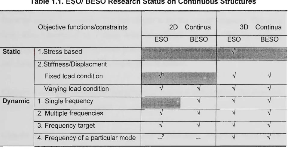
1998; Rong et al 2000b). For 2D and 3D continuous stmctures, the research status is

shown in Table 1.1, where the shaded areas are already covered, and the ticked items are

contributions of this thesis.

Table 1.1. ESO/ BESO Research Status on Continuous Structures

Static

Dynamic

Objective functions/constraints

1.Stress based

2.Stiffness/Displacment Fixed load condition Varying load condition 1. Single frequency 2. Multiple frequencies 3. Frequency target

4. Frequency of a particular mode

2D ESO Continua BESO V^ V V V __2 V V V V — 3D ESO •^ V V V V V V Continua BESO •-# V V V V V V

1. Based on the previous study, an example or two will be examined.

2. 2D structures have less basic mode shape types (axial, bending, etc) than 3D structures (axial, in-plane bending, out-of-plane bending torsion, etc.), thus only the 3D problem is studied in this category.

Another contribution of this thesis is including the manufacturing constraint. The

stmctural optimisation result can be a design of great performance, but may be too

complicated to manufacture. In industries, there is a need to balance the stmctural and

manufacture costs, and the optimisation method developed in this thesis can be a very

practical design tool.

Furthermore, a practical design package is to be user friendly. A user of basic stmctural

(24)

of general guidelines. Such guidelines are results of a parameter study in this thesis.

While ESO/BESO is to date an academic code, the work in this thesis will complement

the previous research outcome, and is significant in its future development into a

commercial design package.

1.4 Layout of the Thesis

The thesis consists of eight chapters. The first two chapters are for introduction and

literature review, respectively. The last chapter is for the overall summary. The main

body from Chapters 3 to 7 deals with three topics: Chapters 3&4 for stiffiiess

optimisation. Chapters 5 for dynamic problems and Chapters 7&8 for parameter studies

and design post-processing. An outline is given as follows.

Chapter 1 discusses the general background of stmctural optimisation. The aims and

significance of the thesis are stated.

Chapter 2 is a literature review on stmctural optimisation. Analytical methods for

optimisation including the differentiation calculus and calculus of variations are briefly

introduced. This is followed by a review on numerical methods including the

mathematical programming, optimality criteria and genetic algorithms. Methods for

shape and topology optimisation of discrete and continuum stmctures are reviewed in

more details. The major part of this chapter is devoted to methods for topology

optimisation of continuum structures, such as the homogenisation design method.

Simplified Isotropic Materials with Penalization (SIMP), soft-kill methods and hard-kill

methods.

Chapter 3 deals with topology optimisation with stiffness requirement for 3D

continuous stmctures using the Evolutionary stmctural optimisation (ESO) and

(25)

mathematical basis of ESO (problem statement and sensitivity analysis), computer

algorithms and implementations. A number of examples are given and results are

compared with available benchmarks. Conclusions are drawn regarding effectiveness

and efficiency of the ESO/BESO method.

Chapter 4 is on a special type of stiffness optimisation where a changing loading

condition is considered. Three factors can cause such changes. The first is the

transmissible loading where the exact load location is not known but only a loading

action line is prescribed. The second is the surface loading where the location of loading

depends on the outer shape of stmctures. The third is the inclusion of self-weight in

stmctural analysis. ESO/BESO can be easily adapted to these problems with minor

modifications on the problem statement and/or sensitivity calculation. Examples on 2D

and 3D are presented.

Chapter 5 is for optimisation considering dynamic respects. The ESO/BESO method is

used to address natural frequency optimisation with different objective functions,

namely, to maximise a single frequency, to maximise multiple frequencies and to obtain

a prescribed set of frequencies. They can be generalised in terms of sensitivity number.

Also, three special topics are dealt with including the repeated eigenvalues, closely

spaced eigenvalues and tracking a desired mode shape. A range of examples of 2D plane

stress and 3D continua are presented to demonstrate the feasibility and effectiveness of

the proposed method.

Chapter 6 investigates a number numerical aspects associated with ESO/BESO,

including the reliability of sensitivity analysis and parameter studies. Another attempt is

on design post-processing.

Chapter 7 deals with optimisation with non-stmctural constraints. One of many such

constraints is the perimeter constraint on the optimal design. The investigation is

motivated by reducing the mesh dependency of ESO and BESO algorithms as well as

(26)

technique can achieve the above objectives. Though mesh independency can be still

observed in 3D structures, the perimeter control technique remains its strength of

reducing stmctural configuration.

Chapter 8 draws the conclusions of the investigation of this _ thesis. Further

(27)

Chapter 2 Overview of Structural Optimisation

This chapter reviews the development in the field of structural optimisation. Sect. 2.1

presents the basic mathematical formulation of the optimisation problem, on which

analytical methods such as differential calculus and calculus of variations are

formulated. Numerical methods are reviewed in Sect. 2.2, including the mathematical

programming (MP), optimality criteria (OC) and genetic algorithms (GA). While those

methods have been readily applied to size optimisation, shape and topology

optimisations, are more involved and are presented in detail in Sect, 2,3. This section

consists of two sub-sections. Sect. 2.3.1 deals with shape and topology optimisation of

discrete stmctures and Sect. 2.3.2 is on continuum stmctures. In Sect 2.3.2, shape

optimisation on continua using boundary variation approach is briefiy introduced. The

remainder of this sub-section reviews the topology optimisation regarding topology

description, design variables and problem statement. Various solution routines are

grouped into three groups: those based on homogenisation, evolutionary methods and

hybrid methods. Typical methods in those groups are introduced and their strengths and

weaknesses are discussed. Towards the end, the application of stmctural optimisation as

(28)

Chapter 2. Overview of Structural Optimisation.

2.1 Mathematical Formulation of Optimisation Problems

2.1.1 Mathematic Statement

The optimisation problem can be mathematically interpreted as determining the

extremum (usually, the minimum) of functions subject to certain constraints (Haftka and

Giirdal 1992), i.e.

Minimise / ( x ) . (2.1a)

Such that ^.(x) = 0,J = 1,...,«,, (2,1b)

hj{x)>0,j = n^ + l,...,n^, (2.1c)

x < x < x , (2-1 d)

where x is the vector of design variables and/(x) is the objective function. gj{x) and

hj{x) are equality and inequality constraints, thus the problem is called constrained

optimisation. Similarly, problems without constraints are called unconstrained

optimisation. Equation (2.Id) is the side constraint where x and x are the lower and

upper bounds of design variables.

In stmctural optimisation, the objective function f{x) is usually chosen to be the

criterion/criteria representing the stmctural volume, weight, cost, performance,

serviceability or their combinations. Constraints gj{x) or hj{x) can be imposed on

stmctural behaviour such as stress, displacement or mean compliance. They can also be

limitations on the functionality and manufacturing tolerance, such as requirements on

the number of stmctural components or cross-sectional dimensions. Design variables

are independent quantities which define a stmcture system and can be modified to

obtain an optimal solution.

(29)

Chapter 2. Oven/lew of Structural Optimisation.

Size optimisation: the design variable can be the thickness of plates or shells, cross

sectional properties of bars, beams or columns, either being the section area or the

moment of inertia, etc.

Shape optimisation: It mainly deals with modification of stmctural geometry.

Geometrical variables can be the coordinates of member joints in discrete stmctures, the

length and location of supports of beam stmctures and the height of shell stmctures.

Shape optimisation for continuous stmctures is usually performed by varying existing

boundaries.

Topology optimisation: for discrete skeletal stmctures such as tmsses, frames or

honeycombs, topology optimisation is also known as layout optimisation. It is used to

determine the pattem of member connection as well as the number and spatial sequence

of nodes and elements. Both size and geometrical variables can be involved. For

continuous stmctures, the optimal topology design is to find the optimum profile of

extemal and intemal boundaries. Topology optimisation is usually accompanied by size

and shape optimisations and is the most difficult and challenging task among the three,

as will be firrther discussed in Sect. 2.3.

2.1.2 Analytical Approaches

Differential Calculus

In differential calculus, conditions for existence of extreme values are stated as that the

first order of derivative of objective functions with respect to the design variable is

equal to zero, i.e.

(30)

The solution vector {Xy,X2,...,x„} to the system of equations constitutes the extreme

points.

The above situation can only be applied to very simple cases of unconstrained

optimisation. For equality constrained optimisation, there are two techniques for

deriving the necessary conditions. Firstly, if the constraint equation can be solved to

obtain the relationship between dependent design variables, the constrained problems

are transformed into unconsfrained ones. Secondly, in cases where constraints are

implicit functions of design variables, a general method called Lagrangian multiplier

can be used, i.e. an auxiliary ftmction using the Lagrangian multiplier Xj is formulated

as follows:

L{x,X) = f{x) + t,Xjgj (2.3)

J=x

with the necessary conditions of an extremum expressed as

dL

— = 0, z = l,.

OXi

dL

. , « ,

•.«e

(2.4)

Optimisation is to solve the above system of equations with altogether n+ n^ unknowns.

The number of Lagrangian multipliers n^ is equal to that of constraints.

For a general class of problems with both equality and inequality constraints, the

necessary condition for an extremum is summarised as the Kuhn-Tucker conditions,

which can be expressed in a simple form as:

(31)

The complementary slackness conditions are needed to consider in the above equation

and the Lagrangian multipliers for inequality constraints A.^ {j =n^+l ,...,n) are

required to be greater than zero.

Calculus of Variations

It is a generalisation of the differentiation theory. It deals with optimisation problems

having an objective function /expressed as a definite integral of a functional F defined

by an unknown function >^ and some of its derivatives (Haftka and Gurdal 1992).

The objective ftmction can be defined as

**^ = ^(^'^'f'-^>*' (^•^>**

where y is directly related to the design variable x. Optimisation is to find the form of

function y = y{x) instead of individual extreme points.

Analogous to the case of differential calculus, the necessary condition for an extremum

is the vanish of the first order of variation, i.e.

8 / = f f ^ + ~ + . . . U = 0. (2.7)

"ydy oy J

Applying boundary conditions, after arrangement, equation (2.7) can be finally

expressed in form of Euler-Lagrange Equation as follows:

dF_ d_

(32)

Chapter 2. Oven/iew of Structural Optimisation.

with the natural boundary conditions {x=a and x=b):

dy' 0, and = 0 (2.8b)

The differential calculus and calculus of variations emphasize the analytical exploration

of optimisation problems. Their earliest application to stmctural design might be due to

Maxwell (1895) in designing the least weight layout of frameworks. The later research

on the optimal topology of tmsses by Michell (1904) was well known as Michell type

stmctures. Except for those results, the application of classical analytical methods is

very limited because of the mathematical complexity and impractical idealisations.

Nonetheless, analytical methods are of fundamental importance in that they explore the

mathematical nature of optimisation and provide the lower bound optimum against

which the results by altemative methods can be checked.

2.2 Basic Numerical Algorithms

2.2,1 Mathematical Programming

Mathematical programming (MP), initially formulated in 1950s (Heyman 1951), can be

the most popular optimum search technique. It starts from an initial design defined by a

selected set of design variables. An improved design is searched in the direction of

gradient of behaviour functions in the form of Lagrangian auxiliary functions. At each

step, the value of behaviour function of a new stmctural design is evaluated. Design

variables are modified gradually until the objective function achieves convergence.

At the earlier stage, the mathematical programming method is limited to linear problems

where the objective functions and constraints are linear functions of design variables. In

1960s, nonlinear programming (NLP) was integrated with finite element analysis as

first suggested by Schmit (1960). Since then, numerous algorithms of nonlinear

(33)

gradient projection (Rosen 1961), penalty function methods (Fiacco and McCormick

1968) and generalised geometric programming (CGP) (Avriel and William 1970), Each

technique can suit a certain type of problems. For example, CGP combined with a

monomial treatment can handle problems with a large number of mixed equality

/inequality constraints (Bums 1987).

2.2.2 Optimality Criteria

Optimality criteria (OC) method was analytically formulated by Prager and co-workers

(Prager and Shield 1968; Prager and Taylor 1968). It is then developed numerically and

becomes a widely accepted stmctural optimisation method (Venkayya et al. 1968). It

also adopts concepts of objective functions and constraints and defines a prior criterion.

The optimum is achieved when the criterion is satisfied. Defining such a criterion may

take advantage of special design conditions and engineering judgement.

In general, most of OC algorithms consist of four fimdamental steps: stmctural analysis,

stating criteria, scaling and resizing.

The Kuhn-Tucker condition constitutes the optimality criteria:

Ze^.X. = l, i = l,2,...,n, (2.9)

Where eij = —^ / — , is the Lagrangian energy density, and L is the Lagrangian

dxj I dXj

multiplier. Equation (2.9) means that in an optimal design, the weighted sum of

Lagrangian energy density is the same for all structural elements. The equation can be

transferred to a recurrence formula to resize the design variable.

The mathematical programming and optimal criteria methods are the two best

(34)

featured by its mathematical elegance and generality. It is less problem specific and is

particularly suitable for problems of multiple constraints problem. However, the

computational cost increases dramatically when a large number of constraints or design

variables are considered. This somehow limits its application to large size stmctures. In

contrast, optimality criteria method is less size dependent and offers ^-bigh convergence

speed. Although the convergence may become unstable, especially in the case of

inappropriately defined initial designs, the relatively low computational cost of OC

makes it particularly appealing for large stmctural systems.

These two methods are reconciled, to a large extent, by formulating dual MP methods

(Fleury 1979), which can be interpreted as generalised OC methods. In dual methods,

the constrained primary minimisation problem is transformed into the maximisation of a

quasi-unconstrained dual function which is only related to the Lagrangian multipliers.

When the primal problem is convex, explicit and mathematically separable, use of dual

methods is very effective by introducing some intermediate design variables. Based on

the use of reciprocal design variable, the convex linearisation method (CONLIN)

(Fleury and Braibant 1986) was well developed, and was later generalised as the method

of moving asymptotes (MMA) (Svanberg 1987). As dual methods search the optimum

direction in the space of Lagrangian multipliers instead of that of the primal design

variables, it can save considerable computing efforts when the number of constraints is

smaller than that of design variables.

2.2.3 Genetic Algorithms

Genetic algorithms (GA), as originally developed in 1970s (Holland 1975), has been

extended to solve the stmctural optimisation problems (Goldberg 1989). Its principle

uses Darwinian's theory of survival of the fittest and adaptation. The procedure consists

of reproduction, crossover and mutation. In the beginning, an initial population of

designs (individuals) is randomly created, with design variables represented by a code

of bit strings. The fitness of each individual is evaluated according to a fitness function.

(35)

in a new generation with member having higher degree of most favourable

characteristics than the parent generation. This process repeats until the best individual

of the population reaches a near-optimum solution.

Genetic algorithms may not be as efficient as traditional MP or OC methods because

they are quite computationally intensive. Nonetheless, they still serve as reliable and

robust techniques for their merits. Compared to the gradient-based search methods,

genetic algorithms search the solution more extensively in that it involves a set of

candidate solutions (individuals). They work on the objective function itself rather than

its derivatives and is more likely to converge to a global optimum. Furthermore, genetic

algorithms fransfer design variables into a code representation, typically, into a binary

bit-string, which is integer in nature. Therefore, it is highly potential for problems

involving a mix of continuous, discrete and integer design variables, such as

optimisation of composite stmctures (Nagendra et al. 1993; Le Riche and Haftka 1994).

When using the above MP, OC and GA algorithms to perform size optimisation, i.e.

changing the size variables, aspects as to design variable, objective and constraints

poses no particular problems. Indeed, size optimisation has been well addressed and

reached a mature level, both in research and industrial applications. Recently, there has

been increasing interest in shape and topology optimisation and this is fiirther discussed

in the following sections.

2.3 Current Methods for Shape and Topology Optimisation

Compared to size optimisation, shape and topology optimisations are more complicated

due to difficulties associated in parameterising the optimisation problems. The design

variable for describing the geometry or topology is not straightforward. Also, the

variable may not be explicit in expressing the objective function and constraint. In this

section, methods are reviewed on optimisation of discrete stmctures and continuum

(36)

2.3.1 Layout Optimal Design for Discrete Structures

Topology optimisation for discrete stmcture is referred to as optimal layout design. The

topic has its origin in Michell's least weight design of tmss stmctures (Michell 1904).

His work has been fiirther developed by Prager and Rozvany and the results are well

knovm as the layout theory (Prager and Rozvany 1977; Rozvany 1989). A survey on

this topic is give by Topping (1993).

In layout optimisation, there are size variables (the section property) and geometry

variables (e.g. the coordinator of stmctural joints). In the geometry approach (Schmit

1960), the number of joints and connecting members is fixed unless some joint coalesce

leads to change in the structural configuration. As the mixed design variables can be of

magiutude of rather different orders, it may cause difficulties in overall convergence.

This leads to the formulation of the hybrid approach (Vanderplaats and Moses 1972).

The size and geometrical variables can be divided into two design spaces and

accordingly, there are two steps in updating design variables.

The most recent approach might be the ground structural approach. A ground stmcture

consists of a dense set of nodes and a large number of potential connections between

those nodes. The number and position of nodes are fixed while the number and size of

connecting elements are altered. Size variables are still continuous, but if the section

area of some elements reduces to zero during optimisation, these elements are deleted

from the stmcture and the stmctural topology changes accordingly.

2.3.2 Shape and Topology Optimisation for Continuous Structures

2.3.2.1 Boundary variation approach to shape optimisation

The stmctural shape .boundary, either extemal or intemal, can be represented by

parameters, and the shape optimisation is described by moving the boundary. There are

(37)

boundary shapes, generation of finite element mesh and solution strategies (Bennett and

Botkin 1986; Haftka and Grandhi 1986).

The description of boundary shapes is essential to the boundary variation approach.

There are several ways to represent the boundary, such as the boundary nodes,

polynomials and splines. In the survey by Ding (1986), different ways are compared in

respects of design variable selection, numerical accuracy and optimal shape. For the

numerical implementation of the boundary variation approach, a capability of automated

mesh refinement is indispensable. The refinement can be undertaken either globally by

re-dividing the whole stmcture or locally by introducing additional elements or

increasing the order of finite elements.

The above boimdary variation method only modifies stmctural boundaries which are

existing. It is not able to remove an existing boundary or create a new one, thus

precludes changes in the connectivity of the stmctural geometry. The optimal design has

the same topology as the initially given topology, which somehow restricts the optimal

solution. In fact, any fine tuning of the stmctural boundary cannot offset an improperly

defined topology.

In topology optimisation, the topology in not known in prior, but is allowed to change

during the solution procedure. The final design may be significantly different from the

initial guess. Topology optimisation can generally produce designs of improved

performance and lower cost than the shape optimisation.

2.3.2.2 Ground structure approach to topology optimisation

Topology optimisation has been a topic of extensive research in the last two decades.

While algorithms such as mathematical programming and optimal criteria are well

developed, the complexity in topology optimisation firstiy lies in the description of the

topology and definition of design variable. Use of parameterised geometry as in the

(38)

Chapter 2. Oven/iew of Structural Optimisation

different shape, dimensions and numbers. For this limitation, methods for topology

optimisation are largely based on the concept of a ground stmcture.

In a continuum setting, let Q be the given candidate design domain consisting of the

loading and displacement boundary conditions. The topology optimisation consists of

finding the sub-domain Q^ of Q , with the prescribed volume K * in which a given

objective function / i s extremised. In other words, the connectedness, the shape and

number of holes are to be decided in the design domain. If one defines the material

density as the design variable, the optimisation problem can be written as

Minimise / ( p ) . (2.10a)

Subject to g=^pdx<V*, (2.1 Ob)

p(x) = 0 o r l , x 6 Q . (2.10c)

In a finite element model of the continuum, the density at each node is taken as the

design variable, and the problem is translated to:

Minimise / ( p ) . (2.11a)

Subject to g = ^ * - ^ p.x. =0, (2.11b)

;=1

p,e{0,l}, i = l,...,n. (2.11c)

The optimisation problem is thus intrinsically discrete. A natural way to solve it is to

use the genetic algorithms (GA) as the binary design variable is analogous to the 0-1

coding. There are some successful examples, such as optimising of 2D continua

(Chapman et al. 1994). However, in an exhaustive search method, the scale of the

problem solved is limited by the high computing demands. In fact, methods based on a

(39)

Alternatively, the search can be based on heuristics, e.g. stress ratio as adopted in

practical design routine. Those methods can be classified into three groups (Bulman and

Hinton 1999):

1) Those based on the homogenisation theory, or h-based, typically represented by the

homogenisation (Bendsoe and Kikuchi 1988) method and Simplified Isotropic

Material with Penalization (SIMP) (Zhou and Rozvany 1991). In these methods, the

discrete optimisation problem is transferred to a continuous one, by either

introducing micro-structures or assuming continuous densities and interpolation

ftmction.

2) Those based on evolution, or e-based, which are initially developed from the

heuristic concept of fully stressed design (FSD). A design of uniform stress can be

evolved by gradually 'killing' elements of low stress in hard kill methods such as

ESO (Xie and Steven 1993), and in soft-kill methods such as adaptive biologic

growtii (Mattheck 1997). While the soft-kill methods focus on stress-based

optimisation, ESO has been significantly extended to accommodate other design

objectives and constraints. Sensitivity analysis rather than stress ratio is used as the

evolution criteria.

3) Hybrid methods, which shares characteristics of the above two methods, such as the

Constrained Adaptive Topology Optimisation (CATO) (Bulman and Hinton 1999).

The algorithm has the same feature of stress ratio as in the e-based methods, but may

also involve microstmctures as in the h-based methods.

The first two groups form the base of stmctural topology optimisation and the remainder

of this section reviews typical methods in these groups.

(40)

This method assumes that the continuum stmcture includes materials with periodic,

perforated microstmctures. There are many types of microstmctures, such as a square

cell with square hole, a rank-1 layered material and a rank-2 layered material. The

homogenisation theory (Babuska 1976 and 1977) as used for composite material is

applied to compute the material properties, e,g, elasticity tensor. The design variable

used here is the microstmcture orientation and density which are calculated from

microstmcture geometries.

Use of continuous density means that there are three phases of material in the stmcture:

soUd material (1), void (0) and intermediate material (0~1). It is necessary to exclude the

intermediate material and force a manufacturable design of 0-1 density. Techniques for

suppressing the chattering design can be either introducing a priori restriction on the

microstmctures (Suzuki and Kikuchi 1991) or imposing postiori penalty on the

intermediate value of material density (Allaire and Kom 1993),

The homogenisation method has been used successfully since its numerical

implementation first presented by Bens0e and Kikuchi (1988). It has been extended to

optimisation under multiple loads (Diaz and Bens0e 1992) and design of complaint

mechanism (Ananthasuresh et al 1994; Saxena and Ananthasuresh 1998). In stmctural

dynamic design, the method has addressed the eigenvalue problems (Tenek and

Hagiwara 1993; Ma et al 1995), stmctural harmonic response (Ma et al 1993),

transient response (Min et al 1999), and unified static and dynamic designs (Min et al

2000). Apart from 2D problems, 2D plate/shell microstmcture and 3D microstmcttire

have been examined (Kikuchi et al 1991; Diaz and Lipton 1997; Olhoff et al 1998). A

full presentation and detailed bibliographies can be found in books on this topic

(Bends0e 1995; Hassani and Hinton 1999).

Simplified Isotropic Material with Penalization (SIMP)

This method transfers discrete variables to continuous ones by introducing interpolation

(41)

interpreted as material densities p . Physical quantities, say, the elasticity tensor E can

be expressed as:

E{p)=p''E„ (2.12)

where E^ is the elasticity tensor of the fixed material and P is some chosen power.

Unlike in the homogenisation method where p corresponds to a certain microstmcture,

the density here is considered rather as a programming strategy than a realistic material

type. For this reason, the SIMP method has been previously regarded as an 'artificial'

material model. However, it has been proved recently that the approach can be

physically permissible if the power satisfies simple conditions (Bendsoe and Sigmund

1999), e.g. /? > 3 for Poisson's ration equal t o j ,

By using a power greater than one, the stiffness at an intermediate density is penalised

in that a certain amount of material gives less than proportional stiffness (as p < 1). The

power has significant effects on the solution. A reasonable range can be 1.2-4,0. By

increasing the value, the penalty on the intermediate density becomes heavier which

leads to a more distinct black-and-white topology. Also, the value of the penalty

exponent can be varying during iterations and this technique is called the continuation

approach (Jog 1993). Theoretically, a sufficiently high value of P steers solutions to

discrete 0-1 values. In practice, altemative strategies are used in SIMP to obtain a

black-and-white topology, such as the filter technique (Sigmund 1994) and perimeter control

(Haber et al. 1996). A survey on SIMP is given by Sigmund and Petterson (1998).

Soft Kill Methods:

There are various heuristically based methods for topology optimisation using the

concept of 'soft kill'. The objective is normally a fully stressed, or uniform stress

design. This design is obtained by strengtiiening the over-stressed part and decreasing

the under-stressed part, which to some extent mimics the adaptive biological growtii. In

(42)

iteration by setting the value of the element stress. This means that the stronger part

will sustain more loads, and the weaker part will become even weaker and eventually be

'killed'. Similarly, in the cellular automation generation method (Inou et al 1994),

elements of low elasticity modulus are gradually killed by applying some

'birth-and-death' mle.

Hard Kill Methods:

In the above methods, the discrete problem of topology optimisation is replaced with

some continuous approach, by either heuristic rules or some more mathematically

rigorous approaches. In contrast, hard kill methods direct deals wdth the 0-1 discrete

variable.

• Evolutionary Structural Optimisation (ESO)

It is based on the concept that by systematically removing inefficient materials from the

stmcture, the residual shape evolves toward an optimum (Xie and Steven 1993). There

are two kinds of removing criteria, which can be based on a certain average stress or on

the sensitivity number. The former was the original form of ESO and the latter is a

significant extension.

When using the stress as design criteria, a cut-off element stiess is defined as the reject

ratio {RR) times the maximum stress. Elements with stress lower than the cut-off stress

(i.e. a^ <RRiG^^, where / is the iteration step) are removed. This procedure repeats

until there are no elements satisfying the inequality. This means that the cut-off stress

should be increased, and the removal ratio is updated to RR^^^ = RR/ + ER where ER is

the evolution ratio. By this procedure, the stress distribution in the stmcture becomes

more uniform.

There are a few variants in the stress-based approach, such as:

• Nibbling ESO: elements can only be nibbled away from the stmctural boundary and

(43)

• Reduction of stress concentration: shapes of cut-out, hole, joint, etc. are optimised in

order to reduce the maximum stress.

• Thermal stress optimisation: to obtain the optimum design of uniform stress under

the thermal load conditions (Li et al. 1997),

• Elastic contact: the contacting profile of several separate bodies is optimised to

reduce the maximum contact stress (Li et al. 1998).

• Nonlinear problems: stmctures with material and geometric nonlinearities are

investigated where the sfrain energy density is used as the evolution criterion

(Querin ^r a/. 1996).

In the class of ESO based on the sensitivity number, the element removal is based on the

value of element sensitivity, defined as the change in objective functions/constraints as a

result of element to be removed. It is calculated by stmctural sensitivity analysis on the

finite element model, such as the mean compliance sensitivity and eigenvalue

sensitivity. This means that the general solution routine of ESO can be applied to

problems of different objectives/constraints. Indeed, the range of problems solved by

ESO includes the stiffiiess/displacement (Chu 1997), natural frequency (Xie and Steven

1994), stmctural vibration (Rong et al 2001a) and stmctural buckling (Manickarajah et

al 1998). Furthermore, different stmctural systems have been accommodated including

2D and 3D discrete stmcture, 2D plate and 2D and 3D continuum. It is also noted that

size, shape and topology optimisation can be addressed respectively or simultaneously.

One improvement of ESO is its extension to bi-directional ESO (BESO). This is to

allow for both element removal and addition (Querin 1997). It has the advantage of

correcting some prematurely removed elements or admitting new elements. As such, it

can start from a small initial design instead of an over-sized ground stmcture. This can

save computing cost of finite element analysis.

To include non-stmcture constraint is a recent development of ESO/BESO. The ICC

(intelligent cavity control) method can effectively control the number of cavities in

(44)

complexity can be alternatively controlled by bounding the stmctural perimeter and this

is one topic of this thesis.

• Reverse Adaptivity (RA)

The method is based on the same principles as ESO of stress criteria, i.e. removal of

low-stress elements (Reynolds et al. 1999). Its added feature is that procedures of finite

element subdivision and mesh refinement are involved during evolution. The term

'reverse' is used because the subdivision is carried out in the element of low stress

element, as opposed to the conventional finite element adpativity in region of high

stiess. After each finite element analysis, a certain averaged stress is calculated at each

element. The total elements are sorted in a stress-ascending order until the r percent of

the material is the reached and the corresponding stress is the 'cut-off stress. The

elements with stress smaller than the cut-off stress are then subdivided. The subdivision

is based on the element edge length of evolving boundary which is calculated from the

area of the current design and a user-specified number of elements. Take a triangular

element for example, the two element bisection algorithms are adopted for subdivision.

The stmcture is re-analysed based on the refined model and low stressed elements are

re-identified and removed.

Use of an adaptive mesh has a few advantages over the ESO method. Firstiy, the mesh

refinement helps to increase the accuracy of structural response calculation. Although

the stmcture becomes smaller and smaller during evolution, RA ensures that there are

sufficient number of elements to represent the structure. Furthermore, one can start with

a relatively coarse mesh and then successively refine it. This means a much smaller

scale of finite element problems than simply defining a fine mesh from the out-set.

Additionally, the clement refinement results in a fairly smooth stmctural boundary

which make the design highly practical.

The RA algorithms can be semi-automatic or fully automatic. The former includes the

Interactive Design Refinement procedure (IDR) (Christie et al 1998). ft mainly

Evolutionary methods for topology optimisation of continuum structures : static and dynamic problems