Rigorous Upper Bounds on Data Complexities of Block Cipher Cryptanalysis
Subhabrata Samajder and Palash Sarkar Applied Statistics Unit
Indian Statistical Institute
203, B.T.Road, Kolkata, India - 700108. {subhabrata r,palash}@isical.ac.in
Abstract
Statistical analysis of symmetric key attacks aims to obtain an expression for the data complexity which is the number of plaintext-ciphertext pairs needed to achieve the parameters of the attack. Existing statistical analyses invariably use some kind of approximation, the most common being the approximation of the distri-bution of a sum of random variables by a normal distridistri-bution. Such an approach leads to expressions for data complexities which areinherently approximate. Prior works do not provide any analysis of the error involved in such approximations. In contrast, this paper takes a rigorous approach to analysing attacks on block ciphers. In particular, no approximations are used. Expressions for upper bounds on the data complexities of several basic and advanced attacks are obtained. The analysis is based on the hypothesis testing framework. Proba-bilities of Type-I and Type-II errors are upper bounded using standard tail inequalities. In the cases of single linear and differential cryptanalysis, we use the Chernoff bound. For the cases of multiple linear and multiple differential cryptanalysis, Hoeffding bounds are used. This allows bounding the error probabilities and obtain-ing expressions for data complexities. We believe that our method provides important results for the attacks considered here and more generally, the techniques that we develop should have much wider applicability.
AMS Classifications: 94A60, 11T71, 68P25, 62P99
Keywords: block cipher, linear cryptanalysis, differential cryptanalysis, log-likelihood ratio test, hypothesis testing, Chernoff bound, Hoeffding’s inequality.
1
Introduction
Statistical methods are commonly used for analysing attacks on block ciphers and more generally symmetric key ciphers. For an attack that aims at recovering a portion of the secret key, there are three basic parameters of interest. (For a distinguishing attack, the situation is a little different and we consider this later.)
1. The success probabilityPS, i.e., the probability that the correct key will be recovered by the attack.
2. The advantageasuch that the number of false alarms is a fraction 2−aof the number of possible values of the sub-key which is the target of the attack.
3. The data complexity N which is the number of plaintext-ciphertext pairs required to achieve at least a pre-specified success probability and at least a pre-specified advantage.
The main goal of any statistical analysis of an attack is to be able to express the data complexity N in terms of PS and a. All the known methods for doing this, however, provide only approximate expressions forN without
deriving bounds on the approximation errors.
1 INTRODUCTION 2
1.1 Our Contributions
The major motivation of this work is to derive rigorous upper bounds on the data complexity in terms of PS
and a. In particular, we do not use any approximation in the statistical analysis1. To show that this can indeed
be done, we consider five basic cryptanalytic scenarios. These are single linear cryptanalysis; single differential cryptanalysis; multiple linear cryptanalysis; multiple differential cryptanalysis; and the task of distinguishing between two probability distributions. In each case, we show that it is indeed possible to obtain rigorous upper bounds on the data complexity.
The theoretical work is supported by several computations. For the block cipher SERPENT, we use the joint distribution of multiple linear approximations [15] to compute the approximate data complexity given by the analysis in [19] and also the upper bound on data complexity obtained in this work. The ratio of these two values turn out to be between 43 and 63. We further make detailed experimental comparisons of the upper bounds that we obtain to the previously best known approximate values of data complexities using simulated joint distributions. For the cases of single linear cryptanalysis, single differential cryptanalysis and distinguisher, the ratio of the upper bound to the approximate expression is around 10 or smaller. For multiple linear cryptanalysis, the ratio is between 4 and 200. These indicate that the upper bounds that we obtain are not too far away from the approximate values obtained earlier. From a practical point of view, we think it is better to use the upper bound to measure the strength of a cipher, since it may turn out that the approximate data complexities are actually underestimates.
For multiple differential cryptanalysis, however, the upper bound turns out to be much larger than the approximate estimate obtained earlier. The reason for this could be one or both of the following: the approximate value is an underestimate or, the upper bound is an overestimate. Deciding the exact reason requires more work. The data complexity expressions that we obtain are valid for all values of the success probability PS and
advantagea. So, for example, these expressions can be evaluated to obtain data complexities forPS= 0.1. Such
an attack has a 10% chance of being successful and from a cryptanalytic point of view would be considered a valid attack. Similarly, even lower values of PS can be considered. However, in earlier works on multiple linear
cryptanalysis [19] and multiple differential cryptanalysis [11], for the data complexity expressions to be valid, the conditionPS >0.5 is required. This is mentioned in [19] without any explanation. In [11], this condition is
not even mentioned, though, evaluating the expression given there withPS = 0.5 leads to meaningless values of
the data complexity. The condition PS >0.5 is a consequence of using the normal approximation and we refer
to [32] for more details on this issue.
The hypothesis testing based approach is used to analyse the attacks. This requires obtaining the probabilities of Type-I and Type-II errors. In the approximate analysis, the normal approximations are used to conveniently handle these probabilities. We use a different approach. The Type-I and Type-II error probabilities are essentially tail probabilities for a sum of some random variables. There are known rigorous methods for handling such tail probabilities, though, to the best of our knowledge, these methods have not been applied to the hypothesis testing setting.
For the cases of single linear and single differential cryptanalysis, it is required to bound the tail probabilities of a sum of independent Bernoulli distributed random variables. The usual method for handling this is to use the Chernoff bound. Using the Chernoff bound to upper bound the Type-I and Type-II error probabilities quite nicely leads to an expression for the data complexity.
In the cases of multiple linear or multiple differential cryptanalysis, the test statistic is no longer a sum of Bernoulli distributed random variables. As a result, the Chernoff bound does not apply. To tackle these cases, we take recourse to Hoeffding’s inequality. This inequality allows us to bound the required tail probabilities to obtain upper bounds on the Type-I and Type-II error probabilities. The case of distinguisher is tackled similarly. The importance of our work is twofold. On the one hand, we bring an amount of rigour to the statistical treatment of basic block cipher cryptanalysis. More generally, the techniques that we apply have broad
appli-1
1 INTRODUCTION 3
cability and it should be possible to tackle data complexities of other attacks using these techniques. From a practical point of view, our computations confirm that the upper bounds that we obtain are greater than the approximate data complexities reported earlier. Since it is not known whether the approximate values are under or overestimates, we think it is better to use the upper bounds.
1.2 Bounds on Data Complexity
We separately discuss the issue for key recovery attacks and distinguishing attacks.
Case of key recovery attacks: LetNmin(PS, a) be the minimum amount of data required to achieve success
probability at least PS and advantage at least a, where the minimum is over all possible methods of statistical
analysis. Any particular method of statistical analysis provides an expression for the data complexity that is required if the method is followed. Considering a statistical analysis as an algorithmA, letNA(PS, a) denote the
data complexity expression obtained using Ato obtain success probability at least PS and advantage at least a.
ClearlyNA(PS, a) is an upper bound onNmin(PS, a). It is also a lower bound in the sense that at leastNA(PS, a)
amount of data will be required to achieve the parameters PS and aif the methodA is followed.
A boundNA(PS, a) obtained using a statistical methodAis useful to a cryptanalyst. It tells the cryptanalyst
that this amount of data is sufficient to attain success probability at least PS and advantage at least a. Put
another way, a upper bound tells a cryptanalyst that no more data is required to achieve the attack parameters. From a cipher designer’s point of view, a data complexity expression of the type NA(PS, a) is also useful.
It tells the designer that if method A is followed, then at least NA(PS, a) amount of data is required to attain
the parameters PS and a. This provides useful information in quantifying the resistance of the cipher against
a particular type of attack. This is particularly important if A is the best known method for carrying out the statistical analysis. It would be even more useful to a cipher designer to obtain Nmin(PS, a). Unfortunately, to
the best of our knowledge, there is no work in the literature which provides this information.
Case of distinguishing attacks: A distinguishing attack proceeds as a test of hypothesis to distinguish
between two different probability distributions. In this case, the data complexity is considered to be a function of the error probability which is defined to be half the sum of the probabilities of Type-I and Type-II errors. Let Nmin(Pe) be the minimum amount of data required to ensure that the error probability is at mostPe, where the
minimum is over all possible methods of statistical analysis. For a particular statistical method A, letNA(Pe)
be the data complexity required to ensure error probability at most Pe. Similar to the case of key recovery
attacks,NA(Pe) is an upper bound onNmin(Pe) and at leastNA(Pe) amount of data is required to ensure error
probability at most Pe if the method A is followed. Also, the usefulness of NA(Pe) to a cryptanalyst and to a
cipher designer remains the same as in the case of key recovery attacks.
An asymptotic expression for Nmin(Pe) has been described in [4]. The expression is given in terms of the
Chernoff information which involves taking an infimum over all real numbers in (0,1). Consequently, the resulting expression cannot be computed and [4] provides approximations.
To the best of our knowledge, all previously proposed statistical methods either for key recovery attacks or for distinguishing attacks useapproximationsto obtain expressions for data complexity without detailed analysis of the approximation errors. Consequently, the obtained data complexities cannot be considered to be either lower or upper bounds. The present work provides upper bounds on the data complexities and we writerigorous upper bound to emphasise that no approximations are used in our analysis.
1.3 How Good are the Bounds?
1 INTRODUCTION 4
independent random variables. This leads to the question of whether better bounds are known and whether these can be applied to the current context?
The theory of large deviations is concerned with the probability of rare events and so tail probabilities can be handled by this theory. It can be shown that the tail probability is upper bounded by an exponential in N times a function called the rate function. This rate function is the Legendre transform of the moment generating function of the corresponding random variable. In theory, it is indeed possible to express the tail probabilities in terms of the rate function. However, this does not automatically provide meaningful bounds for the data complexity. There are several difficulties involved. For a more detailed discussion of these difficulties, we refer to [33].
1.4 Previous and related works
Linear Cryptanalysis: This was first proposed by Matsui in [26] to cryptanalyze the block cipher DES.
Later Matsui [27] extended this idea by using two linear approximations. In an independent work, Kaliski and Robshaw [22] extended Matsui’s attack involving single linear approximation to ` (≥1) linear approximations. Their result, however, was restrictive as it is required for all` linear approximations to have the same plaintext and ciphertext bits though the key bits could be different.
Biryukov et al [8] further refined the idea of multiple linear cryptanalysis. The authors considered` linear approximations without any assumption on their structure. This, though, also had a restriction. The analysis was valid only for`independent linear approximations. Analysis under the independence assumption was separately done Junod and Vaudenay [21]. Murphy [30] argued that the independence assumption need not be valid.
In a later work, Baign`eres et al [2] used the log-likelihood ratio (LLR) statistic to build an optimal distinguisher between two distributions. This result did not require the independence assumption. The theme of obtaining optimal distinguishers was also investigated in [20, 3].
Sel¸cuk in [34] proposed an order statistics based ranking methodology for analysing single linear and differen-tial cryptanalysis. The paper provided expressions for the data complexity of these attacks. The order statistics based approach uses a well known theorem from statistics to approximate the distribution of an order statistics using the normal distribution. Consequently, the data complexities obtained in [34] are approximate. The order statistics based approach was built upon by Hermelin et al [19]. The authors combined the results obtained in [2, 30, 31, 34] to develop a multilinear cryptanalytic method without the independence assumption.
Differential cryptanalysis: This cryptanalytic method was first proposed by Biham and Shamir in [6]. It
was used to successfully cryptanalyze reduced round variants (with up to 15 rounds) of DES using less than 256 operations. Later in [7], the authors further improved their attack by considering several differentials hav-ing the same output difference. Over time, several variants of differential cryptanalysis have been proposed. These include higher order differentials [24], truncated differentials [23], cube attack [16], boomerang attack [36], impossible differential cryptanalysis [5] and improbable differential cryptanalysis [35].
The general approach to multiple differential cryptanalysis was considered in [10]. This work considered ` differentials having both unequal input and unequal output differences. The case of ` differentials having same input difference but different output differences was analysed in details in [11]. The order statistics based framework was used to derive an expression for the data complexity. A general study of data complexity and success probability of statistical attacks was carried out in [12].
We note that a recent work [32] performs a concrete analysis of normal approximations used in symmetric key cryptanalysis using the Berry-Ess´een theorem. In particular, the work critiques the order statistics based approach advocated by Sel¸cuk [34] and points out several shortcomings. More generally, the entire approach of using normal approximations (without consideration of the error) is questioned.
2 BACKGROUND 5
and can form the basis for future work.
2
Background
In this section, we provide the background for the work. The section starts with a brief background on block cipher cryptanalysis (to the extent necessary for understanding this paper) with emphasis on linear cryptanalysis. Next we provide some details about the important log-likelihood ratio (LLR) test statistics. Appendix A provides relevant details of tail probability inequalities, specifically the Chernoff bound for Poisson trials and the Hoeffding bounds.
2.1 Background for Block Cipher Cryptanalysis
The description of block cipher cryptanalysis given here is tailored towards linear cryptanalysis. Differential cryptanalysis is separately considered later.
A block cipher is a function E : {0,1}k× {0,1}n → {0,1}n such that for each K ∈ {0,1}k, the function
EK(·) ∆
=E(K,·) is a bijection from{0,1}n to itself. HereK is the secret key. Then-bit input to the block cipher
is called the plaintext and then-bit output of the block cipher is called the ciphertext.
Practical constructions of block ciphers have an iterated structure consisting of several rounds. Each round consists of applying a round function parameterised by a round key. The round functions are bijections of{0,1}n.
An expansion function, called the key scheduling algorithm, is applied to the secret key to obtain round keys. Let the round keys be k(0), k(1), . . ., and denote the round functions as R(0)
k(0), R
(1)
k(1), . . .. Further, denote by K
(i)
the concatenation of the first iround keys, i.e., K(i)=k(0)|| · · · ||k(i−1); and letEK(i)(i) denote the composition of the first iround functions, i.e.,
EK(0)(0) = R
(0) k(0); E(i)
K(i) = R
(i−1)
k(i−1)◦ · · · ◦R
(0) k(0) =R
(i−1) k(i−1)◦E
(i−1)
K(i−1), i≥1.
A block cipher may have many rounds and a reduced round cryptanalysis may target only a few of these rounds. Suppose that an attack targets r+ 1 rounds. For a plaintext P, let C be the output afterr+ 1 rounds and B be the output after r rounds. So, B=EK(r()r)(P) and C=R
(r) k(r)(B).
Relations between plaintext and the input to the last round: The basic step in block cipher
cryptanal-ysis is to perform a detailed analcryptanal-ysis of the structure of a block cipher. Such a study reveals one or more possible relations between the following quantities: a plaintextP; the input to the last roundB; and possiblyK(r). Such
relations can be in the form of a linear function or in the form of a differential as we explain later. Usually, such a relation holds only with some probability. The probability is taken over the uniform random choice of P. If there are more than one relation, then it is required to consider the joint distribution of the probabilities that these relations hold. Obtaining relations and their possibly joint distribution is a non-trivial task which requires a great deal of experience and ingenuity. These relations form the bedrock on which a statistical analysis of an attack can be carried out.
Target sub-key: A single relation between P and B will usually involve only a subset of the bits of B. If
2 BACKGROUND 6
the bits of B which are involved in any of the relation between P and B. There are 2m possible choices of the target sub-key bits out of which one is correct and all others are incorrect. The goal is to pick out the correct key.
Setting of an attack: Suppose there areN plaintext-ciphertext pairs (Pj, Cj),j= 1, . . . , N which have been
generated using the correct key and are available. For each choice κ of the last round key bits, it is possible to invert Cj to obtain the relevant bits of Bκ,j. The relevant bits are those which are required to evaluate the
relations discovered in the prior analysis of the block cipher. Note that Bκ,j depends on κ even though Cj may
not. If κ is the correct choice for the target sub-key, thenCj indeed depends on κ, otherwise Cj has no relation
toκ.
GivenPj and the relevant bits of Bκ,j it is possible to evaluate all the known relations. From the results of
these evaluations, a test statistic Tκ is defined. Since there are a total of 2m possible values of κ, there are also
2m random variablesTκ. These random variables are assumed to be independent and the distributions of these
random variables depend on whetherκ is correct or incorrect. It is also assumed that the distributions ofTκ for
incorrect κ are identical. This assumption was considered in [17]. For an attack to be possible, it is required to obtain the two possible distributions of Tκ – one when κ is the correct choice and the other when κ is an
incorrect choice.
2.2 Linear Cryptanalysis
Assume that the analysis of the structure of the block cipher provides ` ≥1 linear approximations. These are given by masks Γ(Pi),Γ(Bi) and Γ(Ki), for i = 1, . . . , `. The subscript P denotes plaintext mask; the subscript B denotes mask afterr rounds; and the subscriptK denotes the mask forK(r). So, ΓP(i)and Γ(Bi) are in{0,1}nand
Γ(Ki) is in {0,1}nr. If ` >1, then the attack is called multiple linear cryptanalysis and if `= 1, we will call the
attack single linear cryptanalysis, or simply, linear cryptanalysis. Define
Li =hΓ(Pi), Pi ⊕ hΓ(Bi), Bi; for i= 1, . . . , `. (1)
Inner key bits: For a fixed but unknown key K(r), the quantity zi = hΓ(Ki), K(r)i is a single unknown bit.
Denote by z = (z1, . . . , z`) the collection of the ` bits arising in this manner. The key masks Γ (1) K , . . . ,Γ
(`) K are
known. So, z is determined only by the unknown keyK(r). The bits represented by z are called the inner key bits. The key K(r) is unknown but, fixed and so there is no randomness in K(r). Correspondingly, z is also
unknown but fixed and there is no randomness in z.
Consider a uniform random choice ofP. The round functions are deterministic bijections and so the uniform distribution onP induces a uniform distribution on B. Each Li is a random variable which can take the values
0 or 1. The randomness of Li arises solely from the randomness ofP. Define the random variable X to be the
following:
X = (L1, . . . , L`). (2)
So, X is distributed over {0,1}` and its distribution is determined by the distribution of theL
i’s which in turn
is determined by the distribution of P.
A single linear approximation is of the form
Li =hΓ(Ki), K(r)i=zi. (3)
Note that we are not assuming any randomness over the key K(r) and the bits zi’s have no randomness even
2 BACKGROUND 7
Joint distribution parameterised by inner key bits: A linear approximation of the type given by (3)
holds with some probability over the uniform random choice of P. The random variables L1, . . . , L` are not
necessarily independent. The joint distribution of these variables is given as follows: For z = (z1, . . . , z`), and
η= (η1, . . . , η`)∈ {0,1}`, define
pz(η) = Pr[L1=η1⊕z1, . . . , L`=η`⊕z`] =
1
2` +η(z) (4)
where−1/2`≤η(z)≤1−1/2`.
The vector ˜pz ∆
= (pz(0), . . . , pz(2`−1)) is a probability distribution, where the integers {0, . . . ,2` −1} are
identified with the set {0,1}`. For each choice of z, we obtain a different distribution. These distributions
are, however, related to each other. Suppose z0 = z⊕β for some β ∈ {0,1}`. Then it is easy to verify that
η(z0) =η⊕β(z). It follows that
pz⊕β(η) = pz(η⊕β). (5)
Let ˜p be the probability distribution ˜p = ˜∆ p0` and under the usual identification of {0,1}` and the integers in
{0, . . . ,2`−1}, write
˜
p = (p0, . . . , p2`−1) (6)
so that for η∈ {0,1}`,p
η =∆p(η) = 1/2`+η.
Notation: There are N plaintext-ciphertext pairs (Pj, Cj) forj = 1, . . . , N. For a choiceκ of the target
sub-key, the Cj’s are partially decrypted to obtain the relevant bits ofBκ,j. For κ∈ {0, . . . ,2m−1}, j = 1, . . . , N
and i= 1, . . . , `, define
Lκ,j,i = hΓ(Pi), Pji ⊕ hΓ(Bi), Bκ,ji; (7)
Xκ,j = (Lκ,j,1, . . . , Lκ,j,`). (8)
2.3 LLR Statistics
Let ˜p= (p0, . . . , pν−1) and ˜q= (q0, . . . , qν−1) be two probability distributions over a finite alphabet of sizeν >0.
The Kullback-Leibler divergence between ˜p and ˜q is defined as follows.
D(˜p||q)˜ =
ν−1
X
η=0
pηln (pη/qη). (9)
The problem of distinguishing between the two distributions is the following. Let X1, . . . , XN be a sequence of
independent and identically distributed random variables taking values from the set {0, . . . , ν−1}. It is known that all the Xi’s follow one of the distributions ˜p or ˜q, but, which one is not known.
The goal is to formulate a test of hypothesis to distinguish between these two distributions. This test takes the form where the null hypothesis “H0: the distribution is ˜p” is tested against the alternate hypothesis “H1:
the distribution is ˜q”.
Note that ˜pis a probability distribution on{0, . . . , ν−1}and the probability at a point η∈ {0, . . . , ν−1}is written as pη. For 1≤j ≤N, the random variableXj takes values from the set {0, . . . , ν −1}. So, the derived
random variable pXj is well defined. One may setWj =pXj. The possible values ofWj are p0, p1, . . . , pν−1. If Xj follows ˜p, then forη ∈ {0, . . . , ν−1}, Pr[Wj =pη] = Pr[Xj =η] =pη; if Xj follows another distribution ˜q,
3 SINGLE LINEAR APPROXIMATION 8
Forj= 1, . . . , N, define
Yj = ln pXj/qXj
. (10)
Let µ0 and σ02 be the mean and variance of Yj under hypothesis H0. Similarly, let µ1 and σ12 be the mean
and variance ofYj under hypothesis H1. Then the expressions for µ0, µ1, σ20 and σ12 can be computed to be the
following.
µ0 =D(˜p||q);˜ µ1=−D(˜q||p);˜
σ02 =Pν−1
η=0p(η)
ln
p(η) q(η)
2
−µ20; σ12 =Pν−1
η=0q(η)
ln
q(η) p(η)
2
−µ21.
)
(11)
The LLR random variable is defined to be the following.
LLR =
N
X
j=1
Yj = N
X
j=1
ln pXj/qXj
=
ν−1
X
η=0
Qηln(pη/qη). (12)
Here Qη = #{j :Xj =η}. Following the method described in [2], it is possible to define a test of hypothesis to
distinguish between the two distributions ˜p and ˜q using approximately
N =
(σ0+σ1)Φ−1(1−Pe)
D(˜p||q) +˜ D(˜q||p)˜
2
(13)
plaintext-ciphertext pairs, where Pe is half the sum of the probabilities of Type-I and Type-II errors and Φ is
the standard normal distribution function. More details are given in the appendix.
3
Single Linear Approximation
In this section, we consider the case of a single linear approximation. Let P1, . . . , PN be N independent and
uniformly distributed plaintexts. For simplicity, in this section, we will writeLinstead of L1 andLκ,j instead of
Lκ,j,1. Since there is a single linear approximation, the joint distribution ˜p reduces to simply a probability value
p= Pr[Lκ,j = 0]6= 1/2 whenκis the correct choice. For an incorrect choice ofκ, it is conventional to assume that
Pr[Lκ,j = 0] = 1/2. For the correct choice ofκ,Lκ,jfollowsBernoulli(p) for allj, wherep= 1/2+= 1/2±||. The
appropriate sign is determined by the correct value of the inner key bitz∗ and we can writep= 1/2 + (−1)z∗||. Under the wrong key hypothesis, for an incorrect choice of κ,Lκ,j followsBernoulli(1/2) for allj.
Let c = 2(p−1/2) = 2(−1)z∗|| and define µ
0 = p = (1 +c)/2 and µ1 = 1/2. The hypothesis testing
framework will be used. The test statistics is Tκ =|Xκ−N µ1|where Xκ =PNj=1Lκ,j.Consider the following
test of hypothesis:
Hypothesis Test-1 (single linear cryptanalysis):
H0: “κ is correct” versus H1: “κ is incorrect.”
Decision rule: Reject H0 ifTκ ≤t.
Proposition 1. Let 0< α, β <1. In Hypothesis Test-1, the value of t can be chosen such that for
N ≥
2
r
lnβ2+
q
3 (1 +|c|) ln α1 2
c2 (14)
3 SINGLE LINEAR APPROXIMATION 9
Proof. The requirement is to show the bound on N given the values of α and β. As is usual in the hypothesis testing framework, we will obtain two equations, one relating α, t and N and another relating β, t and N. Eliminatingt variable between these two equations will provide the expression for N in terms ofα and β.
Note that underH0,E[Xκ] =N µ0 and underH1,E[Xκ] =N µ1. Defineδ0= (|µ0−µ1| −t/N)/µ0.
The decision threshold t will be chosen to satisfy 0 < t/N < |µ0 −µ1|. For t in this range, we have
0 < δ0 < |µ0 −µ1|/µ0 < 1. So, it is possible to apply the Chernoff bound (specifically (40) and (41) of
Theorem 7) with thisδ0.
First supposeµ0 > µ1. Thenδ0= (µ0−µ1−t/N)/µ0 and so (1−δ0)µ0 =µ1+t/N.
Pr[Type-I Error] = Pr[Tκ ≤t|H0 holds] = Pr[−t≤Xκ−N µ1 ≤t|H0 holds]
≤ Pr[Xκ−N µ1 ≤t|H0 holds] = Pr[Xκ ≤t+N µ1|H0 holds]
= Pr[Xκ ≤(1−δ0)N µ0|H0 holds]
≤ exp −N µ0δ20/2
≤exp −N µ0δ02/3
.
Recall thatXκ is the sumLκ,1+· · ·+Lκ,N and underH0, eachLκ,j followsBernoulli(p). So, the last step of the
above calculation follows from the Chernoff bound (Equation (41) in the appendix).
Now suppose that µ1 > µ0. (Note that since p 6= 1/2, the case µ0 = µ1 does not occur.) Then δ0 =
(µ1−µ0−t/N)/µ0 and so (1 +δ0)µ0=µ1−t/N. In this case,
Pr[Type-I Error] = Pr[Tκ ≤t|H0 holds] = Pr[−t≤Xκ−N µ1 ≤t|H0 holds]
≤ Pr[Xκ ≥(1 +δ0)N µ0|H0 holds]≤exp −N µ0δ20/3
The last step follows from the Chernoff bound (Equation (40) in the appendix). The actual bound used in this case is different from that used for the case of µ0> µ1.
A relation involvingα and N is obtained by enforcing
α= exp −N µ0δ02/3
.
This shows that Pr[Type-I Error]≤αirrespective of the values ofµ0 and µ1. From the expressions forαand δ0
and using the fact that 0< t/N <|µ0−µ1|we obtain
t = N× |µ0−µ1| −
p
3N µ0ln(1/α). (15)
The probability of Type-II error is given by,
Pr[Type-II Error] = Pr [Tκ > t|H1 holds ] = Pr [|Xκ−N µ1|> t|H1 holds ]
= Pr [Xκ > t+N µ1|H1 holds ] + Pr [Xκ<−t+N µ1|H1 holds ].
Let
δ1 = t/(N µ1) (16)
so that t/N+µ1 = (1 +δ1)µ1 and−t/N +µ1= (1−δ1)µ1. The analysis of Type-I error shows that 0< t/N <
|µ0−µ1|from which it follows that 0< δ1 <1. Using (42) and (43) of Theorem 7, we obtain
Pr[Type-II Error]≤2 exp −N µ1δ12
.
A relation involving β and N is obtained by enforcing
β= 2 exp −N µ1δ12
= 2 exp −t2/(N µ1)
4 MULTIPLE LINEAR CRYPTANALYSIS 10
This shows that Pr[Type-II Error]≤β. Solving for tin terms ofβ and using 0< t/N <|µ0−µ1|yields
t=
s
N µ1ln
2 β
. (17)
Eliminatingt from (15) and (17), we obtain
N = 2
r
ln2β+
q
3 (1 +c) ln α1 2
c2 . (18)
The two expressions for tgiven by (15) and (17) combined with the condition 0< t/N <|µ0−µ1|gives rise to
two lower bounds on N. It is easy to check that the expression for N given by (18) satisfies both these lower bounds.
Recall that c = 2(−1)z∗||. So, depending on the value of z∗, (18) provides two expressions for N, with the expression for z∗ = 1 being (slightly) greater than the expression for z∗ = 0. Taking z∗ = 1 provides the expression on the right hand side of (14). So, for any N greater than this value, the probabilities of Type-I and Type-II errors are upper bounded byα and β respectively.
4
Multiple Linear Cryptanalysis
We assume the setting and notation explained in Sections 2.1 and 2.2. There are `≥1 linear approximations, κ denotes the choice of the target sub-key and z denotes the choice of the inner key bits. There are N plaintext-ciphertext pairs (P1, C1), . . . ,(PN, CN). For a choice κ of the target sub-key; a choice z = (z1, . . . , z`) of the
inner key bit; j∈ {1, . . . , N}; and 1≤i≤`, define
Lκ,j,i=hΓ(Pi), Pji ⊕ hΓP(i), Bκ,ji; Xκ,j = (Lκ,j,1, Lκ,j,2, . . . , Lκ,j,`);
Yκ,z,j = ln
pz(Xκ,j)/2−`
= ln
2`pz(Xκ,j)
.
Suppose z is the correct choice of the inner key bits. For a particular choice of κ, the random variables Xκ,z,1, . . . , Xκ,z,N are independent and these variables follow either the distribution ˜pz or the distribution
˜
q = (2−`, . . . ,2−`) according asκ is the correct choice orκ is an incorrect choice.
The test statistic is defined to be
LLRκ,z = Yκ,z,1+· · ·+Yκ,z,N =
X
η∈{0,1}`
Qκ,ηln(2`pz(η)) (19)
whereQκ,η = #{j :Xκ,j =η}. Consider the following test of hypothesis:
Hypothesis Test-2 (multiple linear cryptanalysis):
H0: “κ is correct” versus H1: “κ is incorrect.”
Decision rule:
Caseµ0 > µ1: RejectH0 if LLRκ,z≤t,∀z∈ {0,1}`; where t∈(N µ1, N µ0);
4 MULTIPLE LINEAR CRYPTANALYSIS 11
Proposition 2. Let 0< α, β <1. In Hypothesis Test-2, it is possible to choose tsuch that for
N ≥ υ
2{p
ln(2`/β) +p
ln(1/α)}2
2(D(˜p||q) +˜ D(˜q ||p))˜ 2 . (20)
the probabilities of the Type-I and Type-II errors are upper bounded by α and β respectively. Here
υ= max
η∈{0,1}`ln(2
`p
η)− min η∈{0,1}`ln(2
`p η) = ln
maxηpη
minηpη
.
Proof. Under H0, eachYκ,z,j has meanµ0 =D(˜pz||q) while under˜ H1, eachYκ,z,j has meanµ1 =−D(˜q||p˜z). It
is not difficult to prove thatµ0 andµ1 have the same value for allz (see [32] for a proof) and so we simply write
µ0 =D(˜p||q) and˜ µ1 =−D(˜q||p), where ˜˜ p= (p0, . . . , p2`−1) as defined in (6).
We now proceed to analyse the probabilities of Type-I and Type-II errors and derive expressions for the data complexity. While doing this, we avoid using normal approximations. We use Hoeffding’s inequalities (see Appendix A.2) to bound the probabilities of the two types of errors.
Recall that for a fixed value ofκ andz, the random variables LLRκ,z,j (j= 1, . . . , N) are independently and
identically distributed with each random variables taking values from the set {ln(2`p0), . . . ,ln(2`p2`−1)}. This, implies that for a fixed value ofκ and z,
υmin = min η∈{0,1}`ln(2
`p
η)≤LLRκ,z,j ≤ max η∈{0,1}`ln(2
`p
η) =υmax;
for all j = 1, . . . , N. Let, υ = υmax−υmin. Therefore one can use Hoeffding bounds (see Appendix A) on
the sum of independent and identically distributed random variables LLRκ,z = PNj=1LLRκ,z,j; where DN =
PN
j=1(υmax−υmin)2 =N υ2.
We now turn to bounding the error probabilities and obtaining expression for the data complexity. This is done separately for the two cases depending on the relative values ofµ0 and µ1. Letz∗ be the correct choice of
the inner key bits.
Case µ0 > µ1: In this case for t ∈ (N µ1, N µ0), to be determined later, the null hypothesis is rejected if
LLRκ,z≤t for all z∈ {0,1}`. Then,
Pr[Type-I Error] = Pr[LLRκ,z ≤tfor all z|H0 holds]≤Pr[LLRκ,z∗ ≤t|H0 holds]
= Pr[LLRκ,z∗N µ0 ≤ −(N µ0−t)|H0 holds]≤exp
−2(N µ0−t)
2
N υ2
.
The last inequality follows from the Hoeffding’s inequality (see (45) of the appendix). Similarly, the probability of Type-II error is computed as follows.
Pr[Type-II Error] = Pr[LLRκ,z > tfor somez|H1 holds]≤
X
z∈{0,1}`
Pr[LLRκ,z> t|H1 holds]
= 2`·Pr[LLRκ,z > t|H1 holds] = 2`·Pr[LLRκ,z−N µ1 > t−N µ1 |H1 holds]
≤ 2`exp
−2(t−N µ1)
2
N υ2
.
The last inequality follows from the Hoeffding’s inequality (see (44) of the appendix). Define
α= exp
−2(N µ0−t)
2
N υ2
; β = 2`exp
−2(t−N µ1)
2
2N υ2
4 MULTIPLE LINEAR CRYPTANALYSIS 12
Then Pr[Type-I Error] ≤α and Pr[Type-II Error]≤β. The expression for α gives two values for t. Using the upper bound ont, i.e., t < N µ0, the expression forthas to be
√
2t=√2N µ0−υ
p
Nln(1/α). (21)
The lower bound on t, i.e., N µ1 < t provides the following lower bound on N.
N > υ
2ln(1/α)
2(µ0−µ1)2
. (22)
Similarly, the expression for β leads to two values fort and again using the range fort, we obtain
√
2t=√2N µ1+υ
q
Nln(2`/β) (23)
and
N > υ
2ln(2`/β)
2(µ0−µ1)2
. (24)
From (21) and (23), we obtain the expression on the right hand side of (20). The expression for N given by (20) satisfies the bounds in (22) and (24).
Case µ0 < µ1: In this case for t ∈ (N µ0, N µ1), to be determined later, the null hypothesis is rejected if
LLRκ,z> t for all z∈ {0,1}`. Then,
Pr[Type-I Error] = Pr[LLRκ,z≥tfor all z|H0 holds]≤Pr[LLRκ,z∗≥t|H0 holds]
= Pr[LLRκ,z∗−N µ0 ≥t−N µ0|H0 holds]≤exp
−2(t−N µ0)
2
N υ2
.
The last inequality follows from the Hoeffding’s inequality (see (44) of the appendix). Similarly, the probability of Type-II error is computed as follows.
Pr[Type-II Error] = Pr[LLRκ,z < tfor somez|H1 holds]≤
X
z∈{0,1}`
Pr[LLRκ,z< t|H1 holds]
= 2`·Pr[LLRκ,z−N µ1 <−(N µ1−t)|H1 holds]≤2`exp
−2(t−N µ1)
2
N υ2
.
The last inequality follows from the Hoeffding’s inequality (see (45) of the appendix). Further analysis of this case in the manner similar to that done for µ1 < µ0 shows that the expression for N in this case is also given
by (20).
Algorithmically, the test is performed in the following manner. Considerµ0 > µ1, the case forµ0< µ1 being
similar. Initialise a setL to be the empty set. For each κ and z, if LLRκ,z > t, then L ← L ∪ {κ}. At the end,
L contains the list of candidate keys.
We consider the time required for computing LLRκ,z for all values of κ and z. For a fixed κ, the values of
Qκ,η for all η ∈ {0,1}` can be computed in O(`N) time. Given these Qκ,η’s, for any z, the value of LLRκ,z
can be computed in O(2`) additional time; for a fixed κ, given the values ofQκ,η’s, the values of LLRκ,z for all
z∈ {0,1}` can be computed inO(22`) additional time. Thus, the values of LLR
κ,z for allκ∈ {0,1}m and for all
5 SINGLE DIFFERENTIAL CRYPTANALYSIS 13
5
Single Differential Cryptanalysis
Let the n-bit strings δ0, δ1, . . . , δr with δ0 6= 0, be the input differences to the rounds of an r+ 1-round block
cipher. Let P be a plaintext and set P0 = P ⊕δ0. Let, B(0) = P, B(1), . . . , B(r) denote the inputs to round
number 0, . . . , r respectively, i.e., B(i+1) = R(i)
k(i)(B(i)) corresponding to the plaintext P. Further, let B(0)
0 =
P0, B(1)0, . . . , B(r)0 be the inputs to round numbers 0, . . . , rrespectively corresponding to the plaintextP0. Then A = ∧r
i=0(B(i)⊕B(i)0 = δi) denotes the event that the differential characteristic δ0 → δ1 → · · · → δr occurs.
Suppose that for the correct keyK, Pr[A] =p. Notice that as in the case of linear cryptanalysis the randomness also comes from the uniform random choice of P.
As in Section 2.2, we assume that guessing m bits of the key allows the partial decryption of C to obtain B(r). These m bits will constitute the target sub-key and the goal will be to obtain the correct value of the sub-key. Further, as done previously, we will denote a choice of the target sub-key by κ.
Let, D denote the event B(r) ⊕B(r)0 = δr. Further, let Pr[D|A] = p0 and p0 = p+ (1−p)p0. Then for
the correct choice κ of the target sub-key Pr[D] = p0. Since δ0 is not the zero string, P 6= P0. This further
implies that B(i) 6= B(i)0 fori = 1, . . . , r since each round function is a bijection. For incorrect choices of κ, it is assumed that B(r) and B(r)0 correspond to uniform sampling without replacement of two n-bit strings from
{0,1}n. Hence, for incorrect of κ, Pr[D] = 1/(2n−1). Let p
w = 1/(2n−1). In general p0 > pw and we will be
proceeding with this assumption. The analysis for the case p0< pw is similar.
Consider N plaintext pairs (P1, P10), . . . ,(PN, PN0 ) with Pj ⊕Pj0 = δ0 and their corresponding ciphertexts
(C1, C10), . . . ,(CN, CN0 ). For a choice κ of the target sub-key, the attacker obtains (B (r) κ,1, B
(r)0
κ,1), . . . ,(B (r) κ,N, B
(r)0
κ,N)
by partially decrypting (C1, C10), . . . ,(CN, CN0 ) respectively. So, for j = 1, . . . , N, it is possible to determine
whether the condition Bκ,j(r)⊕Bκ,j(r)0 =δr holds.
For a choice κ of the target sub-key, define the binary valued random variables Wκ,1, . . . , Wκ,N as follows:
Wκ,j = 1 ifBκ,j(r)⊕Bκ,j(r)=δr; and Wκ,j = 0 otherwise. If κ is the correct choice, then Pr[Wκ,j = 1] =p0 and if κ
is an incorrect choice, then Pr[Wκ,j = 1] =pw for all j.
The test statistics isTκ=|Xκ−µ1|. Consider the following test of hypothesis:
Hypothesis Test-3 (single differential cryptanalysis):
H0: “κ is correct” versus H1: “κ is incorrect.”
Decision rule: Reject H0 ifTκ ≤t.
Proposition 3. Let 0< α, β <1. In Hypothesis Test-3 it is possible to choose tsuch that for
N ≥
3pp0ln(1/α) +
p
pwln(2/β)
2
(p0−pw)2
. (25)
the probabilities of the Type-I and Type-II errors are upper bounded by α and β respectively.
Proof. Let µ0 = p0 and µ1 = pw. where Xκ = Wκ,1 +· · ·+Wκ,N. Under H0, E[Xκ] = N µ0 and under H1,
E[Xκ] =N µ1.
This setting is almost the same as that for single linear cryptanalysis, the only differences being the facts thatµ1 =pw is not in general 1/2 and the inner key bitz is absent. As a result ofµ1 not being equal to 1/2, for
analysing the Type-II error probability we have to apply slightly different forms of the Chernoff bounds.
The expressions forδ0, δ1, αand the expression fortin terms of αare obtained as in the case of single linear
cryptanalysis to be the following:
δ0 = (|µ0−µ1| −t/N)/µ0;
δ1 = t/(N µ1);
α = exp(−(N µ0δ02)/3);
t = N× |µ0−µ1| −
p
6 MULTIPLE DIFFERENTIAL CRYPTANALYSIS 14
Due to the use of the bounds (40) and (41), the expression forβ changes as does the expression fortin terms of β.
β = 2 exp −N µ1δ12/3
;
t = p3N µ1ln(2/β).
Equating the two expressions fort provides the expression on the right hand side of (25).
To apply the Chernoff bound (see Theorem 7), it is required that 0 < δ0, δ1 < 1. As in Section 3, having
0< t/N <|µ0−µ1| ensures that the conditions on δ0 and δ1 hold. The bound on t leads to two lower bounds
on N and the expression for N given by (25) satisfies these two lower bounds.
6
Multiple Differential Cryptanalysis
Here we consider a version of the multiple differential cryptanalysis, where the attacker usesν r-round differentials all having the same input difference. Suppose that theν r-round differentials for a block cipher are given byn-bit stringsδ0andδ(1)r , . . . , δ(rν); whereδ0 denotes the input difference andδr(i)denotes theithoutput difference. Each
of the δ(ri)’s must be non-zeron-bit strings and soν ≤2n−1. As in the case of linear cryptanalysis, consider an
m-bit target sub-key for somem ≤n. Guessing the value of this sub-key allows the inversion of the (r+ 1)-th round. For a uniform random plaintext P, and a choiceκ of the target sub-key, define a random variable Xκ as
follows:
Xκ =
(
i ifR(κr)−1(EK(r)(P))⊕R
(r)
κ −1(EK(r)(P⊕δ0)) =δ
(i) r−1
0; otherwise. (26)
For 1≤i≤ν, let pi and θ be such that
Pr[Xκ =i] =
pi ifκ is the correct choice;
θ ifκ is an incorrect choice. (27)
Under the wrong key assumption, θ= 1/(2n−1). Further, define
p0 = 1−(p1+· · ·+pν); (28)
θ0 = 1−νθ. (29)
Then both ˜p= (p0, p1, . . . , pν) and ˜θ= (θ0, θ, . . . , θ) are proper probability distributions. For the correct choice
of κ,p0 is the probability that none of the ν differentials hold. Similarly, for an incorrect choice of κ,θ0 is the
probability that none of theν differentials hold. The random variableXκ follows ˜p ifκis the correct choice and
Xκ follows ˜θ ifκis an incorrect choice.
Define another random variableYκ = ln
p
Xκ
θXκ
. Let µ0 =E[Yκ] if Xκ follows ˜p (i.e.,κ is the correct choice)
and let µ1 =E[Yκ] ifXκ follows ˜θ (i.e.,κ is an incorrect choice). Then,µ0 =D(˜p||θ) and˜ µ1 =D(˜p||θ).˜
Consider theN plaintext-ciphertext pairs (P1, C1), . . . ,(PN, CN). For a choice κ of the target sub-key and
j = 1, . . . , N, let Xκ,j be the random variable given by (26) corresponding to (Pj, Cj) and let Yκ = ln
p
Xκ,j
θXκ,j
. The test statistics is defined to be the following.
LLRκ = N
X
j=1
Yκ,j =
X
η∈{0,...,ν}
Qκ,ηln(pη/θη)
6 MULTIPLE DIFFERENTIAL CRYPTANALYSIS 15
Hypothesis Test-4 (multiple differential cryptanalysis):
H0: “κ is correct” versus H1: “κ is incorrect.”
Decision rule:
Caseµ0 > µ1: Reject H0 if LLR≤twhere t∈(N µ1, N µ0);
Caseµ0 < µ1: Reject H0 if LLR≥twhere t∈(N µ0, N µ1).
Proposition 4. Let 0< α, β <1 and N be such that
N ≥ υ
2{p
ln (1/β) +pln (1/α)}2
2(D(˜p||θ) +˜ D(˜θ||p))˜ 2 . (30)
Then the probabilities of the Type-I and Type-II errors in Hypothesis Test-4 are upper bounded by α and β respectively. Here,
υ= max
η∈{0,...,ν}ln(pη/θη)−η∈{min0,...,ν}ln(pη/θη).
Proof. Under H0,E[LLR] =N µ0 while under H1,E[LLR] =N µ1.
HereYκ,1, . . . , Yκ,N are independently and identically distributed random variables taking values from the set
{ln(p0/θ0), . . . ,ln(pν/θν)}. Then, for a fixedκ
υmin = min
η∈{0,1,...,ν}ln(pη/θη)≤Yκ,j ≤η∈{max0,1,...,ν}ln(pη/θη) =υmax;
for all j = 1, . . . , N. Let, υ = υmax− υmin. Therefore, Hoeffding bounds can be applied on the sum of
independently and identically distributed random variables LLRκ =PNj=1Yκ,j; whereDN =N υ2.
The error analysis is carried out separately in the two casesµ0 > µ1 and µ0 < µ1.
Case µ0 > µ1: In this case, N µ1 < t < N µ0. The probabilities of Type-I and Type-II errors are computed as
follows:
Pr[Type-I Error] = Pr [LLRκ≤t|H0 holds] = Pr [LLRκ−Nµ0≤ −(Nµ0−t)|H0 holds]
≤ exp
−2(N µ0−t)
2
N υ2
;
Pr[Type-II Error] = Pr [LLRκ>t|H1 holds] = Pr [LLRκ−Nµ1>t−Nµ1|H1 holds]
≤ exp
−2(t−N µ1)
2
N υ2
.
Here the inequalities given by (45) and (44) have been used. Define
α= exp
−2(N µ0−t)
2
N υ2
; β = exp
−2(t−N µ1)
2
N υ2
.
The equation for α gives two values of t. The range for t eliminates one of the values. Similarly, the equation forβ gives two values of twhere one of the values is eliminated using the range for t. The two allowed values of t are the following.
√
2t = √2N µ0−υ
p
Nln(1/α); (31)
√
2t = √2N µ1+υ
p
Nln(1/β). (32)
Eliminating tfrom equations (31) and (32), we obtain the expression given by the right hand side of (30). The expression fortgiven by (31) has to satisfyN µ1 < tand the expression fortgiven by (32) has to satisfyt < N µ0.
7 RELATING ADVANTAGE TO TYPE-II ERROR PROBABILITY 16
Case µ0 < µ1: The analysis of this case is similar and leads to an expression forN which is the same as that
given by (30).
7
Relating Advantage to Type-II Error Probability
The size of the target sub-key is m bits and there is one correct choice and the rest are incorrect choices. The hypothesis test is carried out independently for each choice κ of the target sub-key. Every time a Type-II error occurs, an incorrect choice gets labelled as a candidate key.
In the previous analyses, we have assumedβ to be an upper bound on the probability of Type-II error. For the present, let us assume that β is indeed the actual probability of Type-II error. In the next section, we will consider the situation whenβ is an upper bound.
Since the probability of Type-II error isβ, the expected number of incorrect keys which gets labelled as a candidate key is β(2m−1). An attack is said to have an a-bit advantage if the size of the list of candidate keys produced by the attack is 2m−a. Equating (2m−1)β = 2m−a, we have that for an attack with a-bit expected advantage
β =
2m 2m−1
2−a. (33)
The right hand side can be approximated by 2−afor moderate values ofm. It is possible to use (33) to substitute 2m/(2m−1)×2−a for β in all the expressions for data complexities that have been obtained previously. This allows the data complexities to be expressed in terms of the expected advantagea.
While relating the expected advantage toβ is sufficient for most purposes, it is possible to say more. One can upper bound the probability that the size of the list of false alarms exceeds a certain threshold. This is done as follows.
For each incorrect choice κ of the target sub-key, define Wκ to be a random variable which takes the value
1 if a Type-II error occurs for this choice of κ; and it takes the value 0 otherwise. Then the random variables Wκ’s are independent Bernoulli distributed random variables having probability of successβ. Let
W = X
κ incorrect
Wκ
and let µ=E[W] =β(2m−1). Using the Chernoff bound (38), we have that for anyδ >0,
Pr [W >(1 +δ)µ]< e
δ
(1 +δ)(1+δ)
!µ
.
Define ssuch thats= (1 +δ)µ which combined withµ=β(2m−1) gives
β = s
(1 +δ) (2m−1). (34)
Usings= (1 +δ)µ, we have
Pr [W > s]<
e s−µ
µ
s µ
s µ
µ
= e
s−µµs
ss =Pβ (say). (35)
It is now possible to say that the probability that the list of false alarms exceeds s is at most Pβ. Since µ is
fixed, fixing Pβ fixes s and then the relations= (1 +δ)µ also fixesδ. Using (34), β can be expressed in terms
8 DISTINGUISHERS 17
8
Distinguishers
Consider the problem of distinguishing between the probability distributions ˜pand ˜q over the set{0, . . . , ν−1}. Let, as in Section 2.3, X1, . . . , XN be independent and identically distributed random variables following either
˜
p or ˜q but, which one is not known. As before, let Yj = ln(pXj/qXj) forj = 1, . . . , N and LLR =Y1+· · ·+YN. Consider the log-likelihood ratio (LLR) based test statistics to design a test of hypothesis to distinguish between ˜p and ˜q.
Hypothesis Test-5 (distinguisher):
H0: “the distribution is ˜p” versusH1: “the distribution is ˜q.”
Decision rule:
Caseµ0 > µ1: Reject H0 if LLR≤twhere t∈(µ1, µ0);
Caseµ0 < µ1: Reject H0 if LLR≥twhere t∈(µ0, µ1).
Proposition 5. Let 0< Pe<1. In Hypothesis Test-5, it is possible to choose t such that for
N ≥ υ
2ln(1/P e)
2(D(˜p||q) +˜ D(˜q||p))˜ 2. (36)
the Type-I and Type-II error probabilities satisfy
Pr[Type-I error] + Pr[Type-II error]≤2Pe.
Here,
υ= max
η∈{0,...,ν−1}ln(pη/qη)−η∈{0min,...,ν−1}ln(pη/qη).
Proof. Under H0, Yj has mean µ0 and variance σ02; while under H1, Yj has mean µ1 and variance σ12. The
expressions for µ0, µ1, σ02, σ21 are given by (11). In the present case, we will not have any use for the variances.
UnderH0,E[LLR] =N µ0while underH1,E[LLR] =N µ1. Also note that for the independently and identically
distributed random variables Y1, . . . , YN, each
υmin= min
η∈{0,1,...,ν−1}ln(pη/qη)≤Yj ≤η∈{0max,1,...,ν−1}ln(pη/qη) =υmax.
Let, υ=υmax−υmin. Therefore, Hoeffding bounds can be applied on the sum of independently and identically
distributed random variables LLR =PN
j=1Yj; whereDN =N υ2.
We now consider the probabilities of Type-I and Type-II errors. Since the form of the test is determined by the relative values of µ0 and µ1, the analysis is also done separately.
Case µ0 > µ1:
Pr[Type-I Error] = Pr[LLR≤t|H0 holds] = Pr[LLR−N µ0 ≤ −(N µ0−t)|H0 holds]
≤ exp
−2(N µ0−t)
2
N υ2
.
The last inequality follows from Hoeffding’s inequality (see (45)). Similarly, the probability of Type-II error is computed as follows.
Pr[Type-II Error] = Pr[LLR> t|H1 holds] = Pr[LLR−N µ1 > t−N µ1|H1 holds]
≤ exp
−2(t−N µ1)
2
N υ2
.
9 UPPER BOUNDS 18
Case µ0 < µ1:
Pr[Type-I Error] = Pr[LLR≥t|H0 holds] = Pr[LLR−N µ0 ≥t−N µ0|H0 holds]
≤ exp
−2(t−N µ0)
2
N υ2
.
The last inequality follows from Hoeffding’s inequality (see (44)). Similarly, the probability of Type-II error is computed as follows.
Pr[Type-II Error] = Pr[LLR< t|H1 holds] = Pr[LLR−N µ1 <−(t−N µ1)|H1 holds]
≤ exp
−2(N µ1−t)
2
N υ2
.
The last inequality follows from Hoeffding’s inequality (see (45)). Let
α= exp
−2(N µ0−t)
2
N υ2
; β = exp
−2(t−N µ1)
2
N υ2
.
These expressions are upper bounds on the probabilities of Type-I and Type-II errors respectively irrespective of whether µ0 > µ1 orµ0< µ1.
The quantitiesα and β are determined by N. To obtain a relation betweenPe and N, we set
Pe =
α+β 2 .
Then it follows that (Pr[Type-I Error] + Pr[Type-II Error])≤2Pe.Setting t=N(µ0+µ1)/2 ensuresα=β and
then we obtain the following.
Pe = exp
−2N(µ0−µ1)
2
υ2
= exp
−2N(D(˜p||q) +˜ D(˜q||p))˜
2
υ2
. (37)
From the expression forPe given by (37), the expression forN is given by the right hand side of (36). From this
the statement of the result follows.
9
Upper Bounds
In the previous sections, we have obtained expressions for data complexities. These expressions are in terms of upper bounds on the probabilities of Type-I and Type-II errors.
Letα? and β? be the actual probabilities of Type-I and Type-II errors respectively and further, letα and β be upper bounds onα? andβ? respectively. The success probability isPS? which by definition is 1−α∗. Letting PS= 1−α, we have, PS?≥PS. SettingPS to a pre-specified value ensures that the actual probability of success
PS? is at least this value.
Following the discussion in Section 7, the probability of Type-II error can be related to the expected advantage of an attack. Leta? be such that 2−a?×2m/(2m−1) =β?. Also, definea=−lgβ so that β= 2−a. Then
2−a=β ≥β? = 2−a?×2m/(2m−1)≥2−a?
10 COMPARISON 19
UsingPs = 1−α and β = 2−a all the expressions for the data complexities obtained earlier can be written
in terms ofPS anda.
The main question about data complexity that a cryptanalyst is interested in is the following. For a pre-specified value of PS and a, what is the minimum number of plaintext-ciphertext pairs which ensures that
PS? ≥PS and a? ≥a? Following the discussion in Section 1.2,Nmin(PS, a) denotes this minimum required data
complexity.
The data complexity expressions that we have obtained for the key recovery attacks earlier provide expressions for N in terms of PS and a which can be written as N(PS, a). In other words, this means N(PS, a)
plaintext-ciphertext pairs are sufficient to obtain PS? ≥PS and a?≥a. Again from the discussion in Section 1.2, we have
Nmin(PS, a)≤N(PS, a) for all the cases of key recovery attacks. Similarly, for the case of distinguishing attacks
Nmin(Pe)≤N(Pe). We record these in the following theorem.
Theorem 6. 1. For key recovery attacks using a single linear approximation based on Hypothesis Test-1,
Nmin(PS, a)≤
2np(a+ 1) ln 2 +p3 (1 +|c|) ln (1/(1−PS))
o2
c2 .
2. For key recovery attacks using multiple linear approximations based on Hypothesis Test-2,
Nmin(PS, a)≤
υ2np(a+`) ln 2 +pln (1/(1−PS))
o2
2 (D(˜p||q) +˜ D(˜q||p))˜ 2 .
3. For key recovery attacks using a single differential based on Hypothesis Test-3,
Nmin(PS, a)≤
3nppw(a+ 1) ln 2 +
p
p0ln(1/(1−PS))
o2
(p0−pw)2
.
4. For key recovery attacks using multiple differentials based on Hypothesis Test-4,
Nmin(PS, a)≤
υ2n√aln 2 +pln (1/(1−PS))
o2
2
D(˜p||θ) +˜ D(˜θ||p)˜
2 .
5. For distinguishing attacks based on Hypothesis Test-5,
Nmin(Pe)≤
υ2ln (1/Pe)
2(D(˜p||q) +˜ D(˜q||p))˜ 2.
10
Comparison
Previous works have obtained expressions for data complexities of the various attacks considered in this paper. The analyses have been based on using the central limit theorem to approximate the distribution of the sum of some random variables using the normal distribution. In this work, we have not used any approximation in our analysis. It is of interest to compare the rigorous upper bounds on data complexities that we have obtained with the expressions for data complexities using normal approximations.
10 COMPARISON 20
Let ˜p$ ∆
= (2−`, . . . ,2−`) be the uniform probability distribution over{0,1}`. The variances in case of multiple
linear cryptanalysis will be denoted by (σ0(L))2 and (σ1(L))2 (see [32] for further details). For multiple differential cryptanalysis we denote the variances by (σ0(D))2 and (σ(1D))2 (see [32] for further details). Lastly, for the LLR distinguisher we denote the variances by (σ(Dist)0 )2 and (σ1(Dist))2 (see [32] for further details) The expressions are all similar and our use of different notation is only for the sake of convenience in comparison.
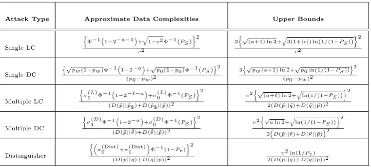
Table 1 compares the expressions for the approximate data complexities that exist in the literature to the corresponding upper bounds on the data complexities obtained in this paper. For single linear and single differential cryptanalysis, the approximate expressions for data complexities were originally obtained in [34]. The approximate expression for the data complexity of multiple linear cryptanalysis was obtained in [19] while the approximate expression for the data complexity of multiple differential crypanalysis was obtained in [11]. These expressions were obtained using the order statistics based approach. In [32], the hypothesis testing framework was used to analyse data complexities. The actual forms of the approximate expressions for the data complexities listed in Table 1 are from [32]. For the case of distinguisher, the original analysis based on normal approximation was done in [2]. This was recapitulated in Section 2.3 and the approximate expression for the data complexity listed in Table 1 is given by (13).
The main observation from Table 1 is that in each case, the denominator of the approximate expression is the same as that of the upper bound. So, the difference between the approximate expression and the upper bound arises from the difference in the numerator. An analytical comparison of the numerators is infeasible. So, we perform an experimental comparison.
Attack Type Approximate Data Complexities Upper Bounds
Single LC
Φ−11−2−a−1+
q
1−c2 Φ−1(PS)2 c2
2
√
(a+1) ln 2+
q
3(1+|c|) ln(1/(1−PS)) 2
c2
Single DC
n√
pw(1−pw)Φ−1
1−2−a
+√p0 (1−p0 )Φ−1(PS)o2
(p0−pw)2
3
n√
pw(a+1) ln 2+√p0 ln(1/(1−PS))
o2
(p0−pw)2
Multiple LC
σ(1L)Φ−1
1−2−`−a
+σ(0L)Φ−1(PS) 2
(D( ˜p||p˜$ )+D( ˜p$||p˜))2
υ2
√
(a+`) ln 2+
q
ln(1/(1−PS)) 2
2(D( ˜p||q˜)+D( ˜q||p˜))2
Multiple DC
σ(1D)Φ−1
1−2−a
+σ(0D)Φ−1(PS) 2
(D( ˜p||θ˜)+D( ˜θ||p˜))2
υ2
√
aln 2+
q
ln(1/(1−PS)) 2
2D( ˜p||θ˜)+D( ˜θ||p˜)2
Distinguisher
σ(Dist)0 +σ(Dist)1
Φ−1 (1−Pe)
2
(D( ˜p||q˜)+D( ˜q||p˜))2
υ2 ln(1/Pe) 2(D( ˜p||q˜)+D( ˜q||p˜))2
Table 1: Table giving the upper bound on the data complexities along with the existing data complexities. Here LC denotes linear cryptanalysis and DC denotes differential cryptanalysis.
10.1 Comparison for SERPENT
10 COMPARISON 21
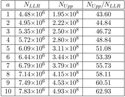
Notice that in order to generate the full joint distribution it is required to get the biases for all the 210−1 = 1023 non-zero linear approximations, generated from the 10 basis linear approximations. Since, only 64 out of these 1023 linear approximations were given in [15], the authors of [18, 19] used two different techniques to generate the full distribution. We have used the second method. Following [19] the value of PS was fixed to
0.95. Table 2, summarises the output of the experiment for a= 1, . . . ,10. In the table, NLLR denotes the data
complexity given by Equation (38) of [19] and NU pp denotes the upper bound for multiple linear cryptanalysis
given in Theorem 6. From the table, it follows that the upper bound on the data complexity is about 43 to 63 times that of the approximate value.
a NLLR NU pp NU pp/NLLR
1 4.48×10⁶ 1.95×10⁸ 43.60
2 4.95×10⁶ 2.22×10⁸ 44.84 3 5.35×10⁶ 2.50×10⁸ 46.72 4 5.72×10⁶ 2.80×10⁸ 48.84 5 6.09×10⁶ 3.11×10⁸ 51.08 6 6.44×10⁶ 3.44×10⁸ 53.39 7 6.79×10⁶ 3.79×10⁸ 55.73 8 7.14×10⁶ 4.15×10⁸ 58.11 9 7.49×10⁶ 4.53×10⁸ 60.51 10 7.83×10⁶ 4.93×10⁸ 62.93
Table 2: Table showing comparison betweenNLLR and NU pp for the block cipher Serpent
10.2 Comparisons Using Simulated Joint Distributions
The approximate expressions contain terms of the type Φ−1(x) and the corresponding term in the upper bound ispAln(1/(1−x)) forA= 1,2,3,6. (For x=PS this can be seen directly; the otherx’s are 1−2−a−1, 1−2−a,
1−2−`−a and 1−Pe and the corresponding values of 1/(1−x) are 2a+1, 2a, 2`+a and 1/Pe respectively.) These
terms do not depend on the probability distributions ˜por ˜q.
Comparing Φ−1(x) with pAln(1/(1−x)): For x varying from 1−2−2 to 1−2−100, Figure 1 shows the plots of Φ−1(x),pln(1/(1−x)) andpln(1/(1−x))/Φ−1(x). This shows that for the given range ofx, the ratio
p
ln(1/(1−x))/Φ−1(x) is between 1 and 2. For A = 2,3 or 6, the ratio increases by √A. Figure 2 shows the plots for the ratio pAln(1/(1−x))/Φ−1(x) for A= 1,2,3 and 6.
From these plots we can infer that the difference in the approximate data complexities and the upper bounds arising due to the difference in Φ−1(x) and pAln(1/(1−x)) is only by a small constant.
Comparisons of components depending on actual distributions: Some of the components in the
nu-merators of the expressions given in Table 1 depend on the actual distributions ˜p and ˜q. Performing these comparisons require simulating appropriate distributions. Below, we mention the actual simulations that were done and the corresponding results.
Comparing 1−c2 and 1+ |c |: Clearly, 1−c2 < 1+ | c |. For our computations, we took c in the range (−2−40,2−40) and in this range√1−c2≈1≈p
10 COMPARISON 22
Figure 1: Plots of Φ−1(x), pln(1/(1−x)) andpln(1/(1−x))/Φ−1(x).
Figure 2: Plots ofpAln(1/(1−x))/Φ−1(x) for A= 1,2,3 and 6.
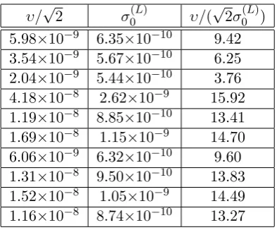
Comparing σ0(L) and σ1(L) withυ/√2: This arises in the case of multiple linear cryptanalysis. For simulating the distributions, we took ` = 5 and randomly selected the probabilities of ˜p in such a way that for all η = 0,1, . . . ,25−1,η ∈(−2−40,2−40). The valuesσ(0L),σ
(L)
1 andυ/
√
2, were then compared by computing the ratios υ/(√2σ0(L)), υ/(√2σ1(L)) and σ0(L)/σ(1L). This experiment was repeated 10 times.
10 COMPARISON 23
υ/√2 σ0(L) υ/(√2σ0(L)) 5.98×10⁻⁹ 6.35×10⁻¹⁰ 9.42 3.54×10⁻⁹ 5.67×10⁻¹⁰ 6.25 2.04×10⁻⁹ 5.44×10⁻¹⁰ 3.76 4.18×10⁻⁸ 2.62×10⁻⁹ 15.92 1.19×10⁻⁸ 8.85×10⁻¹⁰ 13.41 1.69×10⁻⁸ 1.15×10⁻⁹ 14.70 6.06×10⁻⁹ 6.32×10⁻¹⁰ 9.60
1.31×10⁻⁸ 9.50×10⁻¹⁰ 13.83
1.52×10⁻⁸ 1.05×10⁻⁹ 14.49 1.16×10⁻⁸ 8.74×10⁻¹⁰ 13.27
Table 3: Table showing the values of υ/√2,σ0(L) and√2υ/σ0(L).
Comparing σ(0D) and σ1(D) with υ/√2: This arises in the case of multiple differential cryptanalysis. For the simulation we took n = 32, m = 10 and ν = 20 and again ensured that η ∈ (−2−40,2−40) for all η =
0,1, . . . ,20. Random distributions were generated using these parameters like multiple linear cryptanalysis, The ratios √2υ/σ(0D),√2υ/σ1(D) and σ(0D)/σ1(D) were considered. The experiment was also repeated 10 times.
As before the result showed that the ratio √2υ/σ0(D) ≈ √2υ/σ1(D) and σ0(D)/σ(1D) ≈ 1. Table 4 gives the values of υ/√2,σ0(D) and √2υ/σ0(D).
υ/√2 σ0(D) υ/(√2σ0(D)) 0.0071 1.56×10⁻⁷ 32174.65 0.0070 1.51×10⁻⁷ 32578.80 0.0070 1.51×10⁻⁷ 32891.29 0.0066 1.60×10⁻⁷ 28959.21 0.0074 1.44×10⁻⁷ 36168.05 0.0076 1.62×10⁻⁷ 32985.94 0.0077 1.72×10⁻⁷ 31684.23 0.0071 1.44×10⁻⁷ 34608.71 0.0073 1.53×10⁻⁷ 33980.48 0.0074 1.50×10⁻⁷ 34872.68
Table 4: Table showing the values of υ/√2,σ0(D) and√2υ/σ0(D).
The experiment clearly shows that value ofσ(0D) is quite small compared toυ/√2. Reason being, forM = 40 and n = 32, their difference M −n = 8 is quite small. We explain this more clearly. For the distributions considered, we have for all η 6= 0, pη = qη +η, where qη = 1/(2n−1) ≈ 2−n and η ∈ (−2−M,2−M). This
implies,
1−2−(M−n)< pη qη
≈1 + η
2−n <1 + 2
−(M−n).
Therefore, we have
10 COMPARISON 24
which implies thatυis upper bounded by 2−(M−n−1), i.e., 0≤υ <2−(M−n−1). Therefore,υis small if 2−(M−n−1) is small. In the present case we have M = 40 and n= 32, which implies that 2−(M−n−1) = 2−7. Similarly, for multiple linear cryptanalysis υ is upper bounded by 2−(M−`−1). Previously we had taken ` = 10, this makes 2−(M−`−1) = 2−29. This, somewhat explains the reason as to why the value υ/√2 is closer to σ(0L) in case of multiple linear cryptanalysis than compared to σ0(D) for the multiple differential cryptanalysis.
Comparing (σ0(Dist)+σ1(Dist)) with υ/√2: This is relevant for the distinguisher. The distinguisher is defined for arbitrary probability distributions ˜pand ˜q. For the experimental comparison, we applied the distinguisher to the context of multiple linear cryptanalysis. Here, as before, we chose`= 5 andη in the same range as that of
multiple linear cryptanalysis. Unlike the previous cases, here it is required to computeυ/(√2(σ √
2(Dist)
0 +σ
(Dist) 1 )).
As before the experiment was repeated 10 times and the observations are listed in Table 5.
υ/√2 σ0(Dist)+σ1(Dist) √2υ/(σ0(Dist)+σ1(Dist)) 1.33×10⁻⁹ 5.43×10⁻¹⁰ 2.45
2.14×10⁻⁸ 1.40×10⁻⁹ 15.28 4.11×10⁻⁹ 5.81×10⁻¹⁰ 7.08 1.86×10⁻⁹ 5.45×10⁻¹⁰ 3.41
4.35×10⁻⁹ 5.94×10⁻¹⁰ 7.33 4.34×10⁻⁹ 5.76×10⁻¹⁰ 7.55 1.83×10⁻⁸ 1.22×10⁻⁹ 14.96 1.32×10⁻⁹ 5.48×10⁻¹⁰ 2.40 1.98×10⁻⁸ 1.31×10⁻⁹ 15.16 8.10×10⁻⁹ 7.13×10⁻¹⁰ 11.35
Table 5: Table showing the values of υ/√2, (σ(Dist)0 +σ1(Dist)) and√2υ/(σ(Dist)0 +σ1(Dist)).
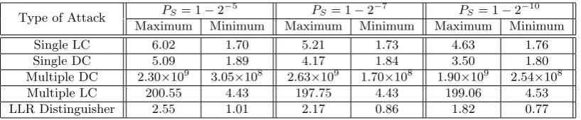
Overall comparison of approximate data complexities with the upper bounds: The size of the target
sub-key was taken to be m = 10 bits and the block size n = 32. For single linear cryptanalysis, we chose c randomly in the range (−2−40,2−40). For single differential cryptanalysis, it was assumed that p0 =pw +c,
wherepw = 1/(2n−1) andcwas chosen randomly from (−2−40,2−40). In the cases of multiple linear cryptanalysis
and the LLR distinguisher we took `= 5 and for multiple differential cryptanalysis we took ν= 20. In all three cases, the η’s were randomly chosen from (−2−40,2−40).
As is normally the case, the success probability PS was fixed to a constant. We have used three different
success probabilities, namely, PS = 1−2−5, 1−2−7 and 1−2−10. The advantage was varied from a = 2 to
100 for all cases other than the LLR distinguisher. For each value of a, the ratio of the upper bound on the data complexity to the approximate data complexity was computed and the minimum and maximum of these values were recorded. The rows of Table 6 reports these minimums and maximums. For the case of the LLR distinguisher, it is required that α =β and hence for our example, a= 5,7 and 10. Since we get a single value of a, we ran the experiment for this value of a100 times for each value ofaand recorded the minimum and the maximum. The last row of Table 6 reports these values.