Performance Evaluation of Relay Selection Schemes
in Beacon-Assisted Dual-hop Cognitive Radio
Wireless Sensor Networks under Impact of Hardware
Noises
Tran Dinh Hieu1,, Tran Trung Duy2,, Le The Dung1and Seong Gon Choi1,∗
1 Department of Radio and Communication Engineering, Chungbuk National University, 362763 Cheongju city, Republic of Korea; [email protected] (T.D.H.); [email protected] (L.T.D.);
[email protected] (S.G.C.)
2 Posts Department of Telecommunications, Posts and Telecommunications Institute of Technology, 70000 Ho Chi Minh City, Vietnam; [email protected]
* Correspondence: [email protected];
† Current address: Chungdae-ro 1, Seowon-Gu, Cheongju, Chungbuk 28644, Building E-10, Room 618 ‡ These authors contributed equally to this work.
Abstract:To solve the problem of energy constraint and spectrum scarcity for cognitive radio wireless sensor networks (CR-WSNs), an underlay decode-and-forward relaying scheme is considered, where the energy constrained secondary source and relay nodes are capable of harvesting energy from a multi-antenna power beacon (PB) and using that harvested energy to forward the source information to the destination. Based on the time switching receiver architecture, three relaying protocols, namely, hybrid partial relay selection (H-PRS), conventional opportunistic relay selection (C-ORS), and best opportunistic relay selection (B-ORS) protocols are considered to enhance the end-to-end performance under the joint impact of maximal interference constraint and transceiver hardware impairments. For performance evaluation and comparison, we derive exact and asymptotic closed-form expressions of outage probability (OP) and throughput (TP) to provide significant insights into the impact of our proposed protocols on the system performance over Rayleigh fading channel. Finally, simulation results validate the theoretical results.
Keywords: energy harvesting; power beacon; decode-and-forward (DF); partial relay selection; opportunistic relay selection; underlay cognitive radio; hardware impairments
1. Introduction
In wireless sensor networks (WSNs), energy is one of the most critical resources because sensors are often low-cost, energy-constrained, resource-constrained nodes [1,2]. The energy harvesting (EH) technique [3,4] has been considering as a viable solution to prolong battery lifetime, improve network performance, and provide green communication for WSNs. Therefore, it has received significant interest from the wireless communication community. Besides conventional EH techniques based on external energy sources such as solar, wind energy, piezoelectric shoe inserts, thermoelectricity, acoustic noise, etc. [5–7], radio frequency (RF) energy harvesting (EH) has recently become a promising technique for WSNs since it allows information and energy to be transmitted simultaneously [8–13]. In [8], the authors first dealt with the fundamental tradeoff between transmitting energy and information at the same time over single input single output (SISO) additive white Gaussian noise (AWGN) channels. Based on these pioneering works, references [9,10] proposed more practical designs, by assuming that the receivers are capable of performing EH and information decoding separately. Zhang and Ho [9] studied multiple input multiple output (MIMO) transmission with practical designs that separate the operation of information decoding and EH receivers. Based on the time switching (TS) and power switching (PS) receiver architectures, references [10,11] proposed two relaying protocols, namely,
time switching-based relaying (TSR) and power switching-based relaying (PSR), to enable EH and information processing at the relay. Following that, references [12,13] showed interest in the application of SWIPT for wireless communication systems. The authors in [12] studied the joint beamforming and power splitting design for a multi-user MISO broadcast system, where a multi-antenna base station (BS) simultaneously transmits information and power to a set of single-antenna mobile stations (MSs). Different from [12], reference [13] considered a large-scale network with multiple transmitter-receiver pairs, where receivers conducted PS technique to harvest energy from RF signals.
Most of the above works focused on EH using radio frequency (RF) transmitted from the source node. However, in practical communication networks, the RF signal is severely degraded due to the huge path loss between the source node and the receiver. Therefore, these systems are only suitable for short distance communications. To overcome this issue, reference [14] proposed a novel hybrid network with randomly deployed power beacons (PB) to provide a practically infinite battery lifetime for mobiles. PB-assisted wireless energy transfer has recently attracted a lot of attention from many researchers [15–17]. The authors of [15] analyzed the throughput of a distributed PB assisted wireless powered communication network via time division multiple access (TDMA) and under i.n.i.d. Nakagami-m fading distribution. The PB-assisted technique has been also studied in the device to device (D2D) communication system [16,17], due to the benefit of D2D systems, i.e., low latency, high spectral efficiency, and low transmit power [18]. In [19,20], multi-hop PB-assisted relaying schemes were studied and investigated. More specifically, the authors in [21,22] proposed novel multi-hop multi-path PB-assisted cooperating networks with path selection methods to enhance the system performance.
Besides energy, another consequence of the explosive growth of wireless services is the spectrum scarcity problem. To solve this problem, the concept of cognitive radio (CR) was first introduced by Mitola in [23], where licensed users (primary users (PUs)) can share their bands to unlicensed users (secondary users (SUs)) provided that quality of service (QoS) of the primary network is still guaranteed. Conventionally, SUs have to periodically sense the presence/absence of PUs, so that they can use vacant bands or move to another spectrum holes [24,25]. In [26,27], various spectrum sensing models for CR WSNs were introduced and compared. References [26,27] also described the advantages of CR WSNs, the main difference between CR WSNs, conventional WSNs, and ad-hoc CR networks. However, the transmission of SUs may be interrupted anytime due to the arrival of PUs, and this is the main disadvantage of the spectrum sensing methods. Recently, underlay CR protocols [28,29] were proposed to guarantee the continuous operation for SUs. In this method, SUs are allowed to utilize the licensed bands simultaneously with PUs provided that the secondary transmitters must adapt transmit power to satisfy an interference constraint given by PUs. To improve the performance of the secondary networks, cooperative relaying protocols [30,31] have been considered as a key technology, due to its capacity to increase the performances gains, i.e., coverage extension or transmission diversity, and power-saving transmission. In the literature, two proactive cooperative relaying strategies that have been widely investigated are opportunistic relay selection (ORS) [31,32], and partial relay selection (PRS) [33,34]. In ORS, the best relay is chosen to maximize the end-to-end (e2e) signal-to-noise ratio (SNR) between source and destination. In PRS, only the channel state information (CSI) of the source-relay links is used to select the relay for the cooperation. However, in [35], the authors proposed a new PRS scheme, where the relay is selected by using CSIs of the relay-destination links. In [35–40], different relay selection schemes in underlay CR networks were reported. Particularly, the authors in [35–37] evaluated the performance of the PRS protocols in terms of bit error rate (BER) and outage probability (OP). In [37–39], the cooperative cognitive schemes using the ORS methods were proposed and analyzed.
multiple channels. Specifically, the authors proposed a system model in which SUs are able to harvest energy from a busy channel occupied by the primary user; the harvested energy is stored in the battery, and it is then used for data transmission over an idle channel. In order to tackle the energy efficiency and spectrum efficiency in CR, an EH-based DF two-way cognitive radio network (EH-TWCR) is proposed in [42]. In particular, the authors proposed two energy transfer policies, two relaying protocols, and two relay receiver structures to investigate the outage and throughput performance. In [43,44], the authors proposed the e2e performance of underlay multi-hop CR networks, where SUs can harvest energy from the power beacon [43] or from the RF signals of the primary transmitter [44].
Next, due to the low-cost transceiver hardware, sensor nodes are suffered from hardware impairments due to phase noise, I/Q imbalance, amplifier nonlinearities, etc. [45–47]. To compensate the performance loss, again cooperative relaying protocols can be employed. Reference [46] investigated the impact of hardware impairments on dual-hop relaying networks operating over Nakagami-m fading channels. In [47], outage probability and ergodic channel capacity of both PRS and ORS methods were measured under joint of co-channel interference and hardware impairments. In [48], the performance of two-way relaying schemes using EH relays with hardware imperfection in underlay CR networks was studied.
1.1. Motivations
In this paper, PB-assisted, hardware impairments, underlay cognitive radio, and cooperative relaying networks are combined into a novel cooperative spectrum sharing relaying system. Our proposed protocols not only improve the energy efficiency, but also the spectrum efficiency for the dual-hop decode-and-forward relaying WSNs. Different from multi-hop PB-assisted relaying schemes [19–22,43,44], this paper considers dual-hop PB-assisted cooperative networks with new relay selection methods. Firstly, we propose a hybrid PRS (H-PRS) protocol which combines the conventional PRS one in [13,34] and the modified one in [35]. Particularly, the scheme in [13,34] is used to select the cooperative relay if it obtains the lower value of OP; otherwise, the scheme in [35] is used. Secondly, to optimize the system performance, we propose a best ORS (B-ORS) protocol which outperforms the conventional ORS (C-ORS) one [32]. Finally, we attempt to evaluate the performance of the H-PRS, B-ORS and C-ORS protocols by providing closed-form expressions of the e2e OP and throughput (TP). The derived expressions are easy-to-compute, and hence they can be used to optimize the system performance.
1.2. Contributions
The main contributions of this paper can be summarized as follows:
• Three dual-hop DF cooperative relaying protocols are proposed. In H-PRS, the best relay can be selected by using the CSIs of the first or second hop. On the other hand, C-ORS and B-ORS select a relay that has the highest e2e channel gain and the highest e2e SNRs, respectively, to convey the data transmission from secondary source to secondary destination.
• It is noteworthy that the PB-assisted cooperative CR relaying systems using H-PRS, B-ORS, or C-ORS have their own mathematical analysis challenges since energy harvested from the beacon and the interference constraint of the primary users (PUs) affect the transmit power of the secondary source and relays. Moreover, due to the correlation between SNRs of the first and second hop, the analysis of the performance in the C-ORS scheme becomes much more challenging, compared with that in the H-PRS and B-ORS ones.
The rest of paper is organized as follows. Section2describes the system model used in this paper. Section3provides the performance evaluation. Section4gives the simulation results, while Section5 concludes the paper.
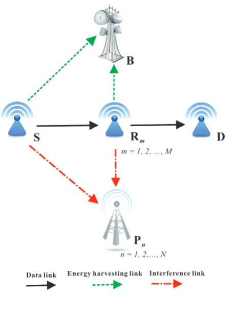
2. System Model
m = 1, 2, ..., M
n = 1, 2,..., N
Figure 1.System model of PB-assisted relaying protocols in underlay CR with relay selection methods. Figure1presents the system model of the proposed CR WSNs. In the secondary network, a source S communicates with a destination D in the dual-hop fashion. In addition, there areMsecondary relays (denoted by R1, R2, ..., RM), and one of them is selected to serve the source-destination communication. In the primary network, there areNlicensed users (or primary users), denoted as P1, P2, ..., PN. To support dynamic spectrum access in a strict manner, the secondary transmitters must adjust their transmit power so that the interferences generated by their operations are not harmful to the quality of service (QoS) of the primary users. It is assumed that the source and relays are single-antenna and energy-constrained devices that have to harvest energy from aK-antenna power beacon (B) deployed in the secondary network. Due to deep shadow fading or far distance, the direct link between S and D does not exist, and the data transmission is realized by two orthogonal time slots via the selected relay.
distribution function (CDF) and probability density function (PDF) of the RVγXYcan be expressed, respectively, as
FγXY(x) =1−exp(−λXYx), fγXY(x) =λXYexp(−λXYx). (1) To take path-loss into account, we can model these parameters as in [30]:
λXY=dβXY, (2)
whereβis the path-loss exponent, anddXYis the link distance between the nodes X and Y.
Assume that the relays (and primary uses) are close together, and form a cluster. Hence,dSRm =
dSR,dSPn =dSPanddRmPn =dRPcan be assumed for allmandn. Hence,γSRm (andγRmD,γSPn,γRmPn) are i.i.d. RVs can be assumed, whereλSRm =λSR,λRmD=λRD,λSPn=λSPandλRmPn =λRPfor allm andn. Similarly,γBkSandγBkRm are also assumed to be i.i.d. RVs, i.e.,λBkS=λBSandλBkRm =λBRfor allkandm.
Next, denote T as the duration of each data transmission from the source to the destination. By using the TSR protocol [11], a duration ofαT is used for the EH process, while the time spent for both
the S-R and R-D transmission is(1−α)T/2, where 0≤α≤1.
2.1. Hardware Impairments
Let us consider the communication between the transmitter X and the receiver Y, the obtained instantaneous SNR of the X-Y link can be formulated by (see [46–48])
Ψ= PXγXY
τX2+τY2PXγXY+N0
= PXγXY
τXY2 PXγXY+N0
, (3)
whereτX2andτY2present levels of the hardware impairments at the transmitter X and the receiver Y,
respectively,τXY2 =τX2+τY2is defined as the total hardware impairment level of the X-Y link, andN0is
a variance of Gaussian noise at Y.
For ease of presentation and analysis, the impairment levels of the data links and interference links are assumed thatτSR2 m =τR2mD=τD2 for allm, andτSP2 n =τR2mPn =τI2for allmandn.
2.2. Energy Harvesting Phase
In this phase, the node B uses all of the antennas to support the energy for the source and the relays. Then, the energy harvested by the source and the relay Rmcan be given, respectively, by (see [15])
QS=ηαTPB
K
∑
k=1γBkS, (4)
QRm =ηαTPB
K
∑
k=1γBkRm, (5)
wherePBis the transmit power of B, andηis the energy conversion efficiency at S and Rm.
From (4) and (5), the average transmit power that the nodes S andRmcan utilize is formulated, respectively, by
ES=
QS
(1−α)T/2 =κPBX
sum
ERm =
QRm
(1−α)T/2 =κPBX
sum
m , (7)
where
κ= 2ηα
1−α,X
sum 0 =
K
∑
k=1γBkS,Xsumm = K
∑
k=1γBkRm. (8)
2.3. Transmit Power Formulation
In underlay CR, the nodes S andRmmust adjust their transmit power to satisfy the interference constraint (see [37]), i.e.,
IS≤
Ith 1+τI2 max
n=1,2,...,N(γSPn)
= Ith
1+τI2Y0max, (9)
IRm ≤
Ith 1+τI2 max
n=1,2,...,N(γRmPn)
= Ith
1+τI2Ymmax
, (10)
whereIthis the interference constraint threshold required by the primary users, and: Y0max= max
n=1,2,...,N(γSPn),Y
max
m = max
n=1,2,...,N(γRmPn). (11)
From (6)-(7), and (9)-(10), the maximum transmit power of S and Rm can be formulated, respectively, as
P0=min(ES, IS) =PBmin
κXsum0 , δ
Y0max
, (12)
Pm =min(ERm, IRm) =PBmin
κXsumm ,
δ
Ymax
m
, (13)
whereδ=Ith/PB/ 1+τI2. In addition, we denoteµ=Ith/PBthat is assumed to be a constant.
Then, under the impact of the hardware impairments, the instantaneous SNR obtained at the first and second hops across the relay can be given, respectively by
Ψ1m=
P0γSRm
τD2P0γSRm+N0
= ∆min κX
sum
0 ,δ/Y0max
γSRm
τD2∆min κXsum0 ,δ/Y0maxγSRm+1
, (14)
Ψ2m=
PmγRmD
τD2PmγRmD+N0
= ∆min(κX
sum
m ,δ/Ymmax)γRmD
τD2∆min(κXsumm ,δ/Ymmax)γRmD+1
, (15)
where∆=PB/N0.
With the DF relaying technique, the e2e channel capacity of the S→Rm→D path is formulated by
Cm=
(1−α)T
2 log2(1+min(Ψ1m,Ψ2m)). (16)
From (16), the e2e outage probability is defined by
whereCthis the target data rate of the secondary network. Then, the e2e throughput (TP) can be formulated as in [11]:
TP= (1−α)TCth(1−OP). (18)
2.4. Relay Selection Methods
2.4.1. Hybrid Partial Relay Selection (H-PRS)
In the conventional PRS protocol [33], the relay providing the highest channel gain at the first hop is selected to forward the data to the destination. Mathematically speaking, we write
Ra1 :γSRa1 = max
m=1,2,...,M(γSRm), (19)
where Ra1is the chosen relay witha1∈ {1, 2, ...,M}.
For the PRS protocol proposed in [35], the best relay is selected by the following strategy:
Ra2 :γRa2D= max
m=1,2,...,M(γRmD), (20)
wherea2∈ {1, 2, ...,M}.
Combining (16)-(17),(19)-(20), the e2e OP of the PRS methods in [33] and [35] can be expressed, respectively as
OPPRS1 =Pr(Ca1 <Cth) =Pr
(1−α)T
2 log2 1+min Ψ1a1,Ψ2a1
<Cth
, (21)
OPPRS2 =Pr(Ca2 <Cth) =Pr
(1−α)T
2 log2 1+min Ψ1a2,Ψ2a2
<Cth
, (22)
In our proposed PRS protocol, if OPPRS1 ≤ OPPRS2, the best relay is selected by (19), and if OPPRS1>OPPRS2, the selection method in (20) is used to choose the relay for the cooperation (the operation of the H-PRS protocol will be described in the next sections). As a result, the outage performance of the H-PRS protocol is expressed as
OPH−PRS=min(OPPRS1, OPPRS2). (23)
Next, the obtained throughput of this protocol is calculated by
TPH−PRS= (1−α)TCth(1−OPH−PRS). (24) 2.4.2. Best Opportunistic Relay Selection (B-ORS)
In the B-ORS protocol, the best relay is chosen to maximize the e2e SNR, i.e.,
Rb:min(Ψ1b,Ψ2b) = max
m=1,2,...,M(min(Ψ1m,Ψ2m)), (25)
Then, the e2e performances of this scheme are given, respectively by
OPB−ORS =Pr
(1−α)T
2 log2(1+min(Ψ1b,Ψ2b))<Cth
,
TPB−ORS = (1−α)TCth(1−OPB−ORS). (26) 2.4.3. Conventional Opportunistic Relay Selection (C-ORS)
As proposed in many literature such as [31,32,38,47], the best relay is selected to maximize the end-to-end SNR of the data link:
Rc:min(γSRc,γRcD) = max
m=1,2,...,M(min(γSRm,γRmD)), (27)
wherec∈ {1, 2, ...,M}.
Then, the e2e OP and e2e TP of the C-ORS protocol is computed as
OPC−ORS =Pr
(1−α)T
2 log2(1+min(Ψ1c,Ψ2c))<Cth
,
TPC−ORS = (1−α)TCth(1−OPC−ORS). (28) It is worth noting that the implementation of C-ORS is simpler than that of B-ORS because it only requires perfect CSIs of the data links.
3. Performance Evaluation
3.1. Outage Probability
Generally, the e2e OP of the protocol U, U∈ {H−PRS, B−ORS, C−ORS}, can be expressed as follows:
OPU=Pr(min(Ψ1l,Ψ2l)<θ) =1−Pr(min(Ψ1l,Ψ2l)≥θ)
=1−Pr(Ψ1l ≥θ,Ψ2l ≥θ), (29)
wherel∈ {a1,a2,b,c}and
θ=2
2Cth
(1−α)T −1. (30)
Moreover, substituting (14) and (15) into (29), which yields
OPU=1−
Pr
1−τD2θ
∆min
κXsum0 , δ
Y0max
γSRl ≥θ,
1−τD2θ
∆min
κXsuml , δ
Ylmax
γRlD≥θ
. (31)
It is obvious from (31) that OPU =1, if 1−τD2θ≤0. In the case that 1−τD2θ>0, equation (31)
can be expressed under the following form:
OPU=1−Pr
min
κXsum0 , δ
Y0max
γSRl ≥
ρ ∆, min
κXsuml , δ
Ylmax
γRlD≥
ρ ∆
, (32)
whereρ=θ/ 1−τD2θ.
OPPRS1=1− K−1
∑
t=0M−1
∑
m=0(−1)m2C
m M−1M
t! (m+1) t−1
2
λBSλSRρ
κ∆
t+1
2
K1−t 2
r
(m+1)λBSλSRρ κ∆
!
−
K−1
∑
t=0N
∑
n=1M−1
∑
m=0(−1)n+m+1CmM−1CnN 2MλSR
t!
ρ
nλSPδ∆+ (m+1)λSRρ
1−2t
λBSρ
κ∆
t+1
2
×K1−t 2
r
λBS
κ∆ (nλSPδ∆+ (m+1)λSRρ)
! × K−1
∑
t=02 t!
λBRλRDρ
κ∆
t+21
K1−t 2
r
λBRλRDρ
κ∆
!
−
K−1
∑
t=0N
∑
n=1(−1)n+1CnN2λRD t!
ρ
nλRPδ∆+λRDρ
1−2t
λBRρ
κ∆
t+21
×K1−t 2
r
λBR
κ∆ (nλRPδ∆+λRDρ)
! , (33)
OPPRS2=1− K−1
∑
t=0M−1
∑
m=0(−1)m2C
m M−1M
t! (m+1) t−1
2
λBRλRDρ
κ∆
t+1
2
K1−t 2
r
(m+1)λBRλRDρ κ∆
!
−
K−1
∑
t=0N
∑
n=1M−1
∑
m=0(−1)n+m+1CmM−1CnN
2MλRD t!
ρ
nλRPδ∆+ (m+1)λRDρ
1−2t
λBRρ
κ∆
t+1
2
×K1−t 2
r
λBR
κ∆ (nλRPδ∆+ (m+1)λRDρ)
! × K−1
∑
t=02 t!
λBSλSRρ
κ∆
t+21
K1−t 2
r
λBSλSRρ
κ∆
!
−
K−1
∑
t=0N
∑
n=1(−1)n+1CnN2λSR t!
ρ
nλSPδ∆+λSRρ
1−2t
λBSρ
κ∆
t+21
×K1−t 2
r
λBS
κ∆ (nλSPδ∆+λSRρ)
! . (34)
Proof. See the proof and notations in Appendix A.
As mentioned in (23), we have OPH−PRS = min(OPPRS1, OPPRS2). In addition, the operation of the H-PRS protocol can be realized as follows. At first, we assume that the source (S) and the destination (D) can know the statistical information of the data links (i.e.,λSR,λRD), the interference links (i.e., λSP,λRP) and the EH links (i.e., λBS,λBR). In practice, the statistical CSIs can be easily obtained by averaging the instantaneous CSI [49,50], and they can be known by all of the nodes via control messages. Next, the source and destination nodes can calculate OPPRS1, OPPRS2by using (33) and (34), respectively. Finally, by comparing OPPRS1and OPPRS2, the source (or the destination) can decide to use the scheme in [33] or in [35] for the source-destination data transmission.
Next, we provide an exact closed-form expression of the e2e OP for the B-ORS protocol as presented in Lemma 2.
OPB−ORS
=1+
K−1
∑
t=0M
∑
m=1(−1)m2C
m M
t! m
λBSλSRρ
κ∆
t+21
Kt−1 2 r
mλBSλSRρ κ∆
!
×
K−1
∑
t=02 t!
λBRλRDρ
κ∆
t+21
K1−t 2
r
λBRλRDρ
κ∆
!
−
K−1
∑
t=0N
∑
n=1(−1)n+1CnN2λRD t!
ρ
nλRPδ∆+λRDρ
1−2t
λBRρ
κ∆
t+21
K1−t 2
r
λBR
κ∆ (nλRPδ∆+λRDρ)
!
m
+
K−1
∑
t=0N
∑
n=1M
∑
m=1(−1)m+n2C
n NCmM
t!
mλBSλSRρ κ∆
t+21
1+nλSPδ∆
mλSRρ
t−21
Kt−1 2 r
λBS
κ∆ (nλSPδ∆+mλSRρ)
!
×
K−1
∑
t=02 t!
λBRλRDρ
κ∆
t+21
K1−t 2
r
λBRλRDρ
κ∆
!
−
K−1
∑
t=0N
∑
n=1(−1)n+1CnN2λRD t!
ρ
nλRPδ∆+λRDρ
1−2t
λBRρ
κ∆
t+21
K1−t 2
r
λBR
κ∆ (nλRPδ∆+λRDρ)
!
m
.
(35)
Proof. See Appendix B.
As presented in Appendix B, the derivation of (35) is different from that of (33) and (34) due to the dependence of the end-to-end SNRs.
Lemma 3. When1−τD2θ>0,OPC−ORScan be expressed by an exact expression as
Proof. See the proof and notations in Appendix C.
OPC−ORS =1
−
M−1
∑
m=0K−1
∑
t=0N
∑
n=0K−1
∑
w=0N
∑
q=0(−1)m+n+qCmM−1 CnNCqN
t!w! λBS κ t λBR κ w
MλRD
λRD+mΩ
×
Z +∞
0 Z z2
0
λBS
κ z
t
1−nλSPδz1t−2−tzt−1 1 λBR
κ z
w
2 −qλRPδzw−2 2−wzw−2 1
×exp
−λSRρ
∆ 1 z1 exp
−(λRD+mΩ)ρ
∆ 1 z2 exp
−λBS
κ z1−
nλSPδ
z1
×exp
−λBR
κ z2−
qλRPδ
z2 dz1dz2 − M−1
∑
m=0K−1
∑
t=0N
∑
n=0K−1
∑
w=0N
∑
q=0(−1)m+n+qCmM−1 CnNCqN
t!w! λBS κ t λBR κ w m m+1
MλSR
λRD+mΩ
×
Z +∞
0 Z z2
0
λBS
κ z
t
1−nλSPδz1t−2−tzt−1 1 λBR
κ z
w
2 −qλRPδzw−2 2−wzw−2 1
×exp
−(m+1)Ωρ
∆ 1 z1 exp
−λBS
κ z1−
nλSPδ
z1
exp
−λBS
κ z2−
qλRPδ
z2
dz1dz2
−
M−1
∑
m=0K−1
∑
t=0N
∑
n=0K−1
∑
w=0N
∑
q=0(−1)m+n+qCmM−1 CnNCqN
t!w! λBS κ t λBR κ w
MλSR
λSR+mΩ
×
Z +∞
0 Z z1
0
λBS
κ z
t
1−nλSPδz1t−2−tzt−1 1 λBR
κ z
w
2 −qλRPδzw−2 2−wzw−2 1
×exp
−λRDρ
∆ 1 z2 exp
−(λSR+mΩ)ρ
∆ 1 z1 exp
−λBS
κ z1−
nλSPδ
z1
×exp
−λBR
κ z2−
qλRPδ
z2 dz1dz2 − M−1
∑
m=0K−1
∑
t=0N
∑
n=0K−1
∑
w=0N
∑
q=0(−1)m+n+qCmM−1 Cn
NC q N
t!w! λBS κ t λBR κ w m m+1
MλRD
λSR+mΩ
×
Z +∞
0 Z z2
0
λBS
κ z
t
1−nλSPδz1t−2−tzt−1 1 λBR
κ z
w
2 −qλRPδzw−2 2−wzw−2 1
×exp
−(m+1)Ωρ
∆ 1 z2 exp
−λBS
κ z1−
nλSPδ
z1
exp
−λBS
κ z2−
qλRPδ
z2
dz1dz2. (36)
Lemma 4. When1−τD2θ>0,OPC−ORScan be approximated by a closed-form expression as given in(37)at the top of next page.
Proof. See the proof and notations in Appendix D.
3.2. Throughput
OPC−ORS ≈1− K−1
∑
t=0M
∑
m=1(−1)m−1C
m M
t!
λSRλBSρ
κ∆
t+21
2mλRD m(λSR+λRD)−λSR
K1−t 2
r
λSRλBSρ
κ∆
!
+
K−1
∑
t=0M
∑
m=1(−1)m−1C
m M
t!
m(λSR+λRD)λBSρ κ∆
t+21
× 2(m−1)λSR
m(λSR+λRD)−λSR
K1−t 2
r
m(λSR+λRD)λBSρ κ∆
!
+
K−1
∑
t=0N
∑
n=1M
∑
m=1(−1)m+n−1C
n NCmM
t!
λBSρ
κ∆
t+21
ρ
nλSPδ∆+λSRρ
1−2t
× 2mλSRλRD
m(λSR+λRD)−λSR
K1−t 2
r
λBS
κ∆ (nλSPδ∆+λSRρ)
!
+
K−1
∑
t=0N
∑
n=1M
∑
m=1(−1)m+n−1C
n NCmM
t!
λBSρ
κ∆
t+21
ρ
nλSPδ∆+m(λSR+λRD)ρ
1−2t
×2m(m−1)λSR(λSR+λRD)
m(λSR+λRD)−λSR
K1−t 2
r
λBS
κ∆ (nλSPδ∆+m(λSR+λRD)ρ)
! × K−1
∑
t=0M
∑
m=1(−1)m−1C
m M
t!
λRDλBRρ
κ∆
t+21
2mλSR m(λSR+λRD)−λRD
K1−t 2
r
λRDλBRρ
κ∆
!
+
K−1
∑
t=0M
∑
m=1(−1)m−1C
m M
t!
m(λSR+λRD)λBRρ κ∆
t+21
× 2(m−1)λRD
m(λSR+λRD)−λRDK1−t 2 r
m(λSR+λRD)λBRρ κ∆
!
+
K−1
∑
t=0N
∑
n=1M
∑
m=1(−1)m+n−1C
n NCmM
t!
λBRρ
κ∆
t+21
ρ
nλRPδ∆+λRDρ
1−2t
× 2mλSRλRD
m(λSR+λRD)−λRD
K1−t 2
r
λBR
κ∆ (nλRPδ∆+λRDρ)
!
+
K−1
∑
t=0N
∑
n=1M
∑
m=1(−1)m+n−1C
n NCmM
t!
λBRρ
κ∆
t+21
ρ
nλRPδ∆+m(λSR+λRD) 1−2t
×2m(m−1)λSR(λSR+λRD)
m(λSR+λRD)−λRD K1−t 2 r
λBS
κ∆ (nλRPδ∆+m(λSR+λRD)ρ)
! . (37)
4. Simulation Results
In this section, a set of numerical results are presented to illustrate the performances of three proposed EH DF cooperative relay selection schemes under the interference constraints of multiple PUs. Monte-Carlo simulations are utilized to verify the theoretical derivations. In the simulation environment, the network nodes are arranged in Cartesian coordinates, where the node S is located at the origin. In addition, the coordinates of the relays, destination, beacon, and primary users are
T=1,N=2 andK=2, respectively. Note that in all simulation results, the simulation results (Sim), the exact theoretical results (Exact) and the asymptotically theoretical results (Asym) are denoted by markers, solid line, and dash line, respectively.
0.1 0.2 0.3 0.4 0.5 0.6 0.7 0.8 0.9
xR
10-4 10-3 10-2 10-1 100
OP
PRS1-Sim (∆=15 dB) PRS2-Sim (∆=15 dB) H-PRS-Sim(∆=15 dB) PRS1-Sim (∆=25 dB) PRS2-Sim (∆=25 dB) H-PRS-Sim(∆=25 dB) PRS1(PRS2)-Exact H-PRS-Exact
Figure 2.Outage probability of the PRS protocols as a function ofxRwhenM=3,xP=0.5,yP=−0.5, α=0.2,Cth=0.5,τD2 =0.1 andτI2=0.05.
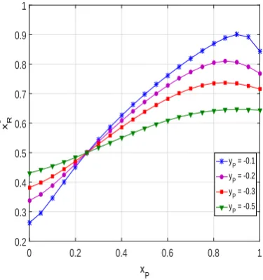
0 0.2 0.4 0.6 0.8 1
xP
0.2 0.3 0.4 0.5 0.6 0.7 0.8 0.9 1
xR
*
yP = -0.1 yP = -0.2 yP = -0.3 yP = -0.5
0 5 10 15 20 25
∆ (dB)
10-4 10-3 10-2 10-1 100
OP
H-PRS-Sim(Cth=0.25) B-ORS-Sim(Cth=0.25) C-ORS-Sim(Cth=0.25) H-PRS-Sim(Cth=0.75) B-ORS-Sim(Cth=0.75) C-ORS-Sim(Cth=0.75) H-PRS-Exact B-ORS-Exact C-ORS-Exact C-ORS-Asym
Figure 4.Outage probability as a function of∆in dB whenM=2,xR =0.5,xP =0.5,yP =−0.5, α=0.25, andτD2 =τI2=0.
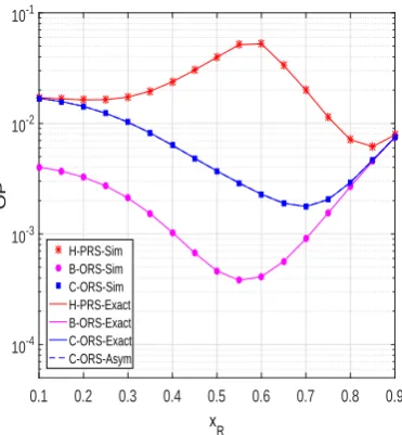
0.1 0.2 0.3 0.4 0.5 0.6 0.7 0.8 0.9
xR
10-4 10-3 10-2 10-1
OP
H-PRS-Sim B-ORS-Sim C-ORS-Sim H-PRS-Exact B-ORS-Exact C-ORS-Exact C-ORS-Asym
Figure 5.Outage probability as a function ofxRwhen∆=20dB,M=4,xP=0.5,yP=−0.5,α=0.1,
Cth=0.6,τD2 =0.1 andτI2=0.05.
equation OPPRS1=OPPRS2(using (33) and (34)), we can find the value ofx∗R. Finally, It is also seen from Fig.2that the outage performance of PRS1, PRS2 and H-PRS is better as increasing the transmit SNR (∆).
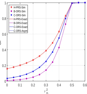
0 0.1 0.2 0.3 0.4 0.5 0.6
τ D 2
0 0.2 0.4 0.6 0.8 1
OP
H-PRS-Sim B-ORS-Sim C-ORS-Sim H-PRS-Exact B-ORS-Exact C-ORS-Exact C-ORS-Asym
Figure 6.Outage probability as a function ofτD2when∆=15 dB,M=5,xR=0.6,xP=0.5,yP=−0.5, α=0.1,Cth=0.7, andτI2=τD2/2.
0.01 0.02 0.03 0.04 0.05
α
0.55 0.6 0.65 0.7 0.75 0.8 0.85
TP
H-PRS-Sim H-PRS-Exact B-ORS-Sim B-ORS-Exact C-ORS-Sim C-ORS-Exact C-ORS-Asym
Figure 7. Throughput as a function ofαwhen∆ =15dB,M = 3,xR =0.5,xP = 0.5,yP =−0.5,
Cth=1, andτI2=τD2 =0.
Figure4compares the outage performance of H-PRS, B-ORS and C-ORS with various values of Cth. We can see that OP of B-ORS is lowest, and OP of H-PRS is highest. At high transmit SNR, OP of B-ORS and C-ORS rapidly decreases as increasing∆. It is due to the fact that B-ORS and C-ORS obtains higher diversity gain as compared with H-PRS.
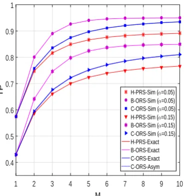
1 2 3 4 5 6 7 8 9 10
M
0.4 0.5 0.6 0.7 0.8 0.9 1
TP H-PRS-Sim (α=0.05)
B-ORS-Sim (α=0.05)
C-ORS-Sim (α=0.05)
H-PRS-Sim (α=0.15)
B-ORS-Sim (α=0.15)
C-ORS-Sim (α=0.15)
H-PRS-Exact B-ORS-Exact C-ORS-Exact C-ORS-Asym
Figure 8. Throughput as a function ofMwhen∆ =20dB,M=3,xR =0.4,xP =0.5,yP =−0.5,
Cth=1,τD2 =0.1 andτI2=0.05.
relay link, thus, H-PRS can be roughly approximated to B-ORS and C-ORS. However, different from B-ORS and C-ORS, the performance of H-PRS is not good as the relays are in the middle of the source and the destination, e.g., OP of H-PRS is highest whenxRis about 0.6.
In Fig.6, we investigate the impact of the hardware impairment level τD2on the performance
of H-PRS, B-ORS and C-ORS. As we can see, the OP values rapidly increase with the increasing of τD2. Moreover, Figure 6shows that all of the proposed protocols are always in outage when τD2 is higher than 0.55. As stated in Section 3, if τD2 ≥ 0.55, then 1−τD2θ < 0, and hence
OPH−PRS=OPB−ORS=OPC−ORS=1.
In Fig.7, the throughput (TP) is presented as a function of the fraction of time allocated for the EH process. As presented in the previous sections, theαvalue plays a key role in the EH process, since
it affects both the harvested power, and the transmit power of the source or the selected relay node. As we can see from this figure, there exists optimal values ofαat which the throughput of the proposed
protocols is highest. This can be explained as follows when theαvalue is too small: less energy can be
harvested from the power beacon. Hence, the small amount of energy that the source or relay node can use for data transmission. At the other extreme, when theαvalue is too large, a less effective
transmission time is utilized to relay the data from source to destination, which leads to the decreasing of the throughput. Therefore, for practical design, the best TP performance can be obtained whenα
reaches the optimal value. Finally, similar to the OP metric, for allαvalues, the TP performance of
B-ORS is always better than that of C-ORS, which further outperforms H-PRS.
Figure8demonstrates TP versus the number of relays. As expected, the throughput of H-PRS, B-ORS and C-ORS can be enhanced by increasing theMvalue. Again, we can see that the performance of the considered protocols can be improved by assigning the value ofαappropriately.
From Figs.4-8, it is evident that the simulation results are perfectly consistent with our derived theoretical values, and the gap between the exact and asymptotic results is small, which verifies the correction of our derivations.
5. Conclusions
operation. We derived exactly and asymptotically the outage probability and throughput of the proposed protocols under the presence of multiple PUs, and over i.i.d. Rayleigh fading channels. The numerical results showed that the performance improvements of B-ORS are higher than those of C-ORS, which in turn, outperforms H-PRS. Finally, the system performance of the proposed protocols can be enhanced by setting an appropriate energy-harvesting ratio, increasing the number of relays, and placing the relays at the advisable position.
Acknowledgments: This work was supported by “Human Resources Program in Energy Technology” of the Korea Institute of Energy Technology Evaluation and Planning (KETEP), granted financial resource from the Ministry of Trade, Industry & Energy, Republic of Korea. (No. 20164030201330).
Author Contributions: The main contributions of Tran Dinh Hieu were to create the main ideas and execute performance evaluation by extensive simulation while Tran Trung Duy, Le The Dung and Seong Gon Choi worked as the advisor of Tran Dinh Hieu to discuss, create, and advise the main ideas and performance evaluations together.
Conflicts of Interest:The authors declare no conflict of interest.
Appendix A: Proof of Lemma1
Firstly, we calculate the outage probability OPPRS1. Due to the independence betweenΨ1a1 and
Ψ1a2, we can rewrite (32) as
OPPRS1=1−Pr
min
κXsum0 , δ
Ymax 0
γSRa1 ≥
ρ ∆
Pr
min
κXsuma1 ,
δ
Ymax
a1
γRa1D≥
ρ ∆
=1−(1−A1) (1−A2), (A-1)
whereA1andA2are outage probability at the first and second hops, respectively, given as
A1=Pr
min
κXsum0 , δ
Ymax 0
γSRa1 <
ρ ∆
,
A2=Pr
min
κXsuma1 , δ
Ymax
a1
γRa1D<
ρ ∆
. (A-2)
Next, we can rewriteA1as
A1= Z +∞
0 FZ1 ρ
∆x
fγSRa1 (x)dx, (A-3)
whereZ1=min
κXsum0 ,Ymaxδ 0
,FZ1(.)and fγSRa1 (.)are CDF and PDF ofZ1andγSRa1, respectively. Combing (1) and (19),FγSRa
1 (.)can be given as
FγSRa1 (x) =Pr
max
m=1,2,...,M(γSRm)<x
= FγSRm(x) M
= (1−exp(−λSRx))M. (A-4)
From (A-4), the corresponding PDF can be obtained as
fγSRa(x) =MλSRexp(−λSRx) (1−exp(−λSRx))
M−1
=
M−1
∑
m=0(−1)mCmM−1MλSRexp(−(m+1)λSRx), (A-5)
Considering the RVZ1; its CDF can be formulated by
FZ1(x) =Pr
min
κX0sum, δ
Ymax 0
<x
=1−1−FXsum 0
x
κ
FYmax
0 δ x . (A-6)
From (8), sinceXsum
0 is sum of i.i.d. exponential RVs, CDFFXsum
0 (x/κ)in (A-6) can be given as FXsum
0 x
κ
=1−exp
λBS
κ x
K−1
∑
t=01 t! λBS κ t
xt. (A-7)
Next, from (11), we can obtain CDFFYmax
0 (δ/x), similar to (A-4), as FYmax
0
δ
x
=1+
N
∑
n=1(−1)nCNn exp
−nλSPδ
x
. (A-8)
Substituting (A-7) and (A-8) into (A-6), we have
FZ1(x) =1− K−1
∑
t=01 t! λBS κ t xtexp
−λBS
κ x
−
K−1
∑
t=0N
∑
n=1(−1)nC
n N t! λBS κ t xtexp
−λBS
κ x−
nλSPδ
x
. (A-9)
Then, substituting (A-5) and (A-9) into (A-3), we arrive at
A1=1−
K−1
∑
t=0M−1
∑
m=0(−1)mCmM−1MλSR t!
λBSρ
κ∆
tZ +∞
0 1 xtexp
−λBSρ
κ∆
1 x
exp(−(m+1)λSRx)dx
−
K−1
∑
t=0N
∑
n=1M−1
∑
m=0(−1)n+mCnNCmM−1 MλSR
t!
λBSρ
κ∆
tZ +∞
0 1 xtexp
−λBSρ
κ∆ 1 x ×exp −
nλSPδ∆
ρ + (m+1)λSR
x
dx. (A-10)
Using [51, eq. (3.471.9)] for the corresponding integrals in (A-10), we obtain
A1=1−
K−1
∑
t=0M−1
∑
m=0(−1)m2C
m M−1M
t! (m+1) t−1
2
λBSλSRρ
κ∆
t+1
2
K1−t 2
r
(m+1)λBSλSRρ κ∆
!
−
K−1
∑
t=0N
∑
n=1M−1
∑
m=0(−1)n+mCmM−1CNn 2MλSR
t!
ρ
nλSPδ∆+ (m+1)λSRρ
1−2t
λBSρ
κ∆
t+1
2
×K1−t 2
r
λBS
κ∆ (nλSPδ∆+ (m+1)λSRρ)
!
. (A-11)
Next, with the same manner as deriving A1, we can obtain an exact closed-form expression for A2 as
A2=1−
K−1
∑
t=02 t!
λBRλRDρ
κ∆
t+21
K1−t 2
r
λBRλRDρ
κ∆
!
−
K−1
∑
t=0N
∑
n=1(−1)nCnN 2λRD
t!
ρ
nλRPδ∆+λRDρ
1−2t
λBRρ
κ∆
t+21
K1−t 2
r
λBR
κ∆ (nλRPδ∆+λRDρ)
!
. (A-12)
Substituting (A-11) and (A-12) into (A-1), we obtain (33). Next, by replacing
λSR,λRD,λBS,λBR,λSPandλRPin (33) byλRD,λSR,λBR,λBS,λRPandλSP, respectively, we can obtain (34).
Appendix B: Proof of Lemma2
From (25) and (29), the e2e OP of the B-ORS protocol is expressed by
OPB−ORS=Pr(min(Ψ1b,Ψ2b)<θ) =Pr
max
m=1,2,...,M(min(Ψ1m,Ψ2m))<θ
. (B.1)
We note that the RVsΨ1m(m=1, 2, ...,M)have a common RV, i.e., Z1 = min
κXsum0 ,Ymaxδ 0
. Hence, we have to rewrite (B.1) under the following form:
OPB−ORS = Z +∞
0 Pr
max
m=1,2,...,M(min(Ψ1m,Ψ2m))<θ|Z1=u
| {z }
B1(u)
fZ1(u)du
=1+
Z +∞
0
∂B1(u)
∂u 1−FZ1(u)
du. (B.2)
Now, we attempt to calculate B1(u)as marked in (B.2):
B1(u) = [Pr(min(Ψ1m,Ψ2m)<θ|Z1=u)]M= [B2(u)]M, (B.3) where
B2(u) =Pr(min(Ψ1m,Ψ2m)<θ|Z1=u) =1−Pr(min(Ψ1m,Ψ2m)≥θ|Z1=u)
=1−Pr
γSRm ≥
ρ ∆u, min
κXsumm , δ
Ymmax
γRmD≥
ρ ∆
=1−1−PrγSRm <
ρ ∆u
(1−A2)
=1−(1−A2)exp
−λSRρ
∆u
. (B.4)
In (B.4), A2is given in (A-12). Next, substituting (B.4) into (B.3), we obtain
B1(u) =1+
M
∑
m=1(−1)mCmM(1−A2)mexp
−mλSRρ
∆u
. (B.5)
Differentiating B1(u)with respect tou, yielding
∂B1(u)
∂u =
M
∑
m=1(−1)mCmMmλSRρ
∆ (1−A2)m 1 u2exp
−mλSRρ
∆u
Substituting (A-9) and (B.6) into (B.2), and then using [51, eq. (3.471.9)] for the corresponding integrals, we can obtain
OPB−ORS=1+
K−1
∑
t=0M
∑
m=1(−1)m2C
m M
t!
mλBSλSRρ κ∆
t+21
(1−A2)mKt−1 2 r
mλBSλSRρ κ∆
!
+
K−1
∑
t=0N
∑
n=1M
∑
m=1(−1)m+n2C
n NCmM
t! m
λBSλSRρ
κ∆
t+21
(1−A2)m
1+ nλSPδ∆
mλSRρ
t−21
×Kt−1 2 r
λBS
κ∆ (nλSPδ∆+mλSRρ)
!
. (B.7)
Next, substituting (A-12) into (B.7), we obtain (35).
Appendix C: Proof of Lemma3
In the C-ORS protocol, the end-to-end OP can be calculated by
OPC−ORS =Pr
min
min
κX0sum, δ
Y0max
γSRc, min
κXcsum, δ
Ycmax
γRcD
< ρ ∆
=Prmin(Z1γSRc,Z2γRcD)<
ρ ∆
=1−Pr
γSRc≥
ρ
∆Z1,γRcD≥
ρ ∆Z2
, (C.1)
whereZ2=minκXsumc ,Ymaxδ c
, and the CDF ofZ2is given, similar toZ1in (A-9):
FZ2(x) =1− K−1
∑
t=01 t!
λBR
κ
t xtexp
−λBR
κ x
−
K−1
∑
t=0N
∑
n=1(−1)nC
n N
t!
λBR
κ
t xtexp
−λBR
κ x−
nλRPδ
x
. (C.2)
SinceγSRcandγRcDare not independent, the method in [47] can be used to calculate OPC−ORS. At first, using [47, eq. (D.2)], we have
Pr(γSRc ≥u1,γRcD≥u2) = Z +∞
0
∂G(z) ∂z
fTmax(z) fTm(z)
dz, (C.3)
where Tm = min(γSRm,γRmD), Tmax = m=max1,2,...,M(Tm), and G(z) = Pr(γSRm≥u1,γRmD≥u2, min(γSRm,γRmD)<z).
Because the CDF ofTmisFTmax(z) =1−exp(−(λSR+λRD)x), its PDF is obtained as
fTmax(z) = (λSR+λRD)exp(−(λSR+λRD)z) =Ωexp(−Ωz), (C.4) whereΩ=λSR+λRD.
Then, the PDF ofTmaxcan obtained, similar to (A-5), as
fTmax(z) = M−1
∑
m=0(−1)mCmM−1MΩexp(−(m+1)Ωz). (C.5)
∂G(z)
∂z =
0, ifz<u2
λRDexp(−λSRu1)exp(−λRDz), ifu2≤z<u1
Ωexp(−Ωz), ifu1≤z
(C.6)
Plugging (C.3)-(C.6) together, and after some manipulations, the following can be obtained:
Pr(γSRc ≥u1,γRcD≥u2|u1≥u2)
=
M−1
∑
m=0(−1)mCmM−1M " Ru1
u2 λRDexp(−λSRu1)exp(−λRDz)exp(−mΩz)dz
+R+∞
u1 Ωexp(−(m+1)Ωz)dz
#
=
M−1
∑
m=0(−1)mCmM−1M " λ
RD
λRD+mΩexp(−λSRu1)exp(−(λRD+mΩ)u2)
+mm+1 λSR
λRD+mΩexp(−(m+1)Ωu1)
#
. (C.7)
• Case 2:u1<u2
∂G(z)
∂z =
0, ifz<u1
λSRexp(−λRDu2)exp(−λSRz), ifu1≤z<u2
Ωexp(−Ωz), , ifu2≤z
(C.8)
Similarly, we obtain
Pr(γSRc ≥u1,γRcD≥u2|u2>u1)
=
M−1
∑
m=0(−1)mCmM−1M
λSR
λSR+mΩexp
(−λRDu2)exp(−(λSR+mΩ)u1)
+ m
m+1
λRD
λSR+mΩ
exp(−(m+1)Ωu2)
. (C.9)
Now, withu1= ∆ρZ
1 andu2= ρ
∆Z2, the following are respectively obtained:
Pr
γSRc ≥
ρ
∆z1,γRcD≥
ρ
∆z2|z2≥z1
=
M−1
∑
m=0(−1)mCmM−1M×
λRD
λRD+mΩ exp
−λSRρ
∆ 1 z1 exp
−(λRD+mΩ)ρ
∆
1 z2
+ m
m+1
λSR
λRD+mΩ exp
−(m+1)Ωρ
∆ 1 z1 , (C.10) Pr
γSRc ≥
ρ ∆z1
,γRcD≥
ρ ∆z2
|z1>z2
=
M−1
∑
m=0(−1)mCmM−1M
λSR
λSR+mΩ exp
−λRDρ
∆ 1 z2 exp
−(λSR+mΩ)ρ
∆
1 z1
+ m
m+1
λRD
λSR+mΩ exp
−(m+1)Ωρ
∆ 1 z2 . (C.11)
Moreover, OPC−ORSin (C.1) can be formulated as
OPC−ORS =1− Z +∞
0 Z z2
0 Pr
γSRc≥
ρ ∆z1
,γRcD≥
ρ ∆z2
|z2≥z1
fZ1(z1)fZ2(z2)dz1dz2
−
Z +∞
0 Z z1
0 Pr
γSRc ≥
ρ ∆z1
,γRcD≥
ρ
∆z2|z1≥z2
where the PDFs ofZ1andZ2can be obtained from their CDFs, i.e.,
fZ1(z1) = K−1
∑
t=0N
∑
n=0(−1)nC
n N
t!
λBS
κ
t
λBS
κ z
t
1−nλSPδzt−1 2−tz1t−1
exp
−λBS
κ z1−
nλSPδ
z1
, (C.13)
fZ2(z2) = K−1
∑
w=0N
∑
q=0(−1)qC
q N
w!
λBR
κ
w
λBR
κ z
w
2 −qλRPδz2w−2−wzw−2 1
exp
−λBR
κ z2−
qλRPδ
z2
. (C.14)
Substituting (C.10), (C.11), (C.13), and (C.14) into (C.12), equation (36) can be obtained, to finish the proof.
Appendix D: Proof of Lemma4
Firstly, relaxing the dependence betweenγSRcandγRcD, we have the following approximation:
OPC−ORS ≈1−Pr
γSRc≥
ρ ∆Z1
Pr
γRcD≥
ρ ∆Z2
≈1−Pr
Z1≥ ρ
∆γSRc
Pr
Z2≥ ρ
∆γRcD
. (D.1)
Our next objective is to calculate PrZ1≥ ∆γSRρ c
and PrZ2≥ ∆γRρcD
, i.e.,
Pr
Z1≥ ρ
∆γSRc
=
Z +∞
0
1−FZ1
ρ ∆y
fγSRc(y)dy,
Pr
Z2≥ ρ
∆γRcD
=
Z +∞
0
1−FZ2
ρ ∆y
fγRcD(y)dy. (D.2)
Using [32, eq. (2)], we obtain PDF ofγSRcandγRcD, respectively as
fγSRc(y) = M
∑
m=1(−1)m−1CmM mλSRλRD m(λSR+λRD)−λSR
exp(−λSRy)
+
M
∑
m=1(−1)m−1CmMm(m−1)λSR(λSR+λRD) m(λSR+λRD)−λSR
exp(−m(λSR+λRD)y),
fγRcD(y) = M
∑
m=1(−1)m−1CmM
mλSRλRD
m(λSR+λRD)−λRDexp
(−λRDy)
+
M
∑
m=1(−1)m−1CmM
m(m−1)λSR(λSR+λRD) m(λSR+λRD)−λRD exp
Combining (A-9) and (D.3), which yields
Pr
Z1≥
ρ ∆γSRc
=
K−1
∑
t=0M
∑
m=1(−1)m−1C
m M
t!
λBSρ
κ∆
t
mλSRλRD m(λSR+λRD)−λSR
×
Z +∞
0 1 ytexp
−λBSρ
κ∆
1 y
exp(−λSRy)dy
+
K−1
∑
t=0M
∑
m=1(−1)m−1C
m M
t!
λBSρ
κ∆
tm(m−1)
λSR(λSR+λRD) m(λSR+λRD)−λSR
×
Z +∞
0 1 ytexp
−λBSρ
κ∆
1 y
exp(−m(λSR+λRD)y)dy
+
K−1
∑
t=0N
∑
n=1M
∑
m=1(−1)m+n−1C
n NCmM
t!
λBSρ
κ∆
t
mλSRλRD m(λSR+λRD)−λSR
×
Z +∞
0 1 ytexp
−λBSρ
κ∆ 1 y exp −
nλSPδ∆
ρ +λSR
y dy + K−1
∑
t=0N
∑
n=1M
∑
m=1(−1)m+n−1C
n NCmM
t!
λBSρ
κ∆
t
m(m−1)λSR(λSR+λRD) m(λSR+λRD)−λSR
×
Z +∞
0 1 ytexp
−λBSρ
κ∆ 1 y exp −
nλSPδ∆
ρ +m(λSR+λRD)
y
. (D.4)
Using [51, eq. (3.471.9)] for the corresponding integrals, and after some manipulations, we obtain
Pr
Z1≥
ρ ∆γSRc
=
K−1
∑
t=0M
∑
m=1(−1)m−1C
m M
t!
λSRλBSρ
κ∆
t+21 2m
λRD m(λSR+λRD)−λSR
K1−t 2
r
λSRλBSρ
κ∆
!
+
K−1
∑
t=0M
∑
m=1(−1)m−1C
m M
t!
m(λSR+λRD)λBSρ κ∆
t+21
× 2(m−1)λSR
m(λSR+λRD)−λSR
K1−t 2
r
m(λSR+λRD)λBSρ κ∆
!
+
K−1
∑
t=0N
∑
n=1M
∑
m=1(−1)m+n−1C
n NCmM
t!
λBSρ
κ∆
t+21
ρ
nλSPδ∆+λSRρ
1−2t
× 2mλSRλRD
m(λSR+λRD)−λSR
K1−t 2
r
λBS
κ∆ (nλSPδ∆+λSRρ)
!
+
K−1
∑
t=0N
∑
n=1M
∑
m=1(−1)m+n−1C
n NCmM
t!
λBSρ
κ∆
t+21
ρ
nλSPδ∆+m(λSR+λRD)ρ
1−2t
×2m(m−1)λSR(λSR+λRD)
m(λSR+λRD)−λSR
K1−t 2
r
λBS
κ∆ (nλSPδ∆+m(λSR+λRD)ρ)
! . (D.5)
Similarly, we can obtain a closed-form expression for PrZ2≥ ρ
∆γRcD
, and then submitting the obtained results into (D.1) to finish the proof.
References
1. Lin, H.; Bai, D.; Gao, D.; Liu, Y. Maximum data collection rate routing protocol based on topology control for rechargeable wireless sensor networks. Sensors 2016, 16, 1201.
3. Jiang, L.; Tian, H.; Xing, Z.; Wang, K.; Zhang, K.; Maharjan, S.; Gjessing, S.; Zhang, Y. Social-aware energy harvesting device-to-device communications in 5G networks. IEEE Wireless Commun. 2016, 23, 20–27. 4. Yadav, A., Goonewardena, M., Ajib, W., Dobre, O. A., Elbiaze, H. Energy management for energy harvesting
wireless sensors with adaptive retransmission. IEEE Trans. Commun. 2017, 65, 5487 - 5498.
5. Paradiso, J. A.; Starner, T. Energy scavenging for mobile and wireless electronics,” IEEE Pervasive Comput. 2005, 4, 18–27.
6. Raghunathan, V. ; Ganeriwal, S.; Srivastava, M. Emerging techniques for long lived wireless sensor networks. IEEE Commun. Mag. 2006, 44, 108–114.
7. Hieu, T. D.; Dung, L. T.; Kim, B.S. Stability-aware geographic routing in energy harvesting wireless sensor networks. Sensors 2016, 16, 1-15.
8. Varshney, L. R. Transporting information and energy simultaneously. In Proc. of IEEE Int. Symp. Inf. Theory (ISIT), Toronto, ON, Canada, Jul. 2008, pp. 1612–1616.
9. Zhang, R.; Ho, C. K. MIMO broadcasting for simultaneous wireless information and power transfer. IEEE Trans. Wireless Commun. 2013, 12, 1989–2001.
10. Zhou, X.; Zhang, R.; Ho, C. K. Wireless information and power transfer: architecture design and rate-energy tradeoff. IEEE Trans. Commun. 2013, 61, 4754–4767.
11. Nasir, A. A.; Zhou, X.; Durrani, S.; Kennedy, R. A. Relaying protocols for wireless energy harvesting and information processing. IEEE Trans. Wireless Commun. 2013, 12, 3622–3636.
12. Shi, Q.; Liu, L.; Xu, W.; Zhang, R. Joint transmit beamforming and receive power splitting for MISO SWIPT systems. IEEE Trans. Wireless Commun. 2014, 13, 3269–3280.
13. Krikidis, I. Simultaneous information and energy transfer in large scale networks with/without relaying. IEEE Trans. Commun. 2014, 62, 900–912.
14. Huang, K.; Lau, V. K. N. Enabling wireless power transfer in cellular networks: Architecture, modeling and deployment. IEEE Trans. Wireless Commun. 2014, 13, 902–912.
15. Le, N.P. Throughput analysis of power-beacon assisted energy harvesting wireless systems over non-identical Nakagami-m fading channels. IEEE Commun. Lett. 2018, 22, 840-843.
16. Liu, Y.; Wang, L.; Zaidi, S. A. R.; Elkashlan, M.; Duong, T. Q. Secure D2D communication in large-scale cognitive cellular networks: A wireless power transfer model. IEEE Trans. Commun. 2016, 64, 329–342. 17. Doan, T. X.; Hoang, T. M.; Duong, T. Q.; Ngo, H. Q. Energy harvesting-based D2D communications in the
presence of interference and ambient RF sources. IEEE Access 2017, 5, 5224-5234.
18. Tehrani, M. N.; Uysal, M.; Yanikomeroglu, H. Device-to-device communication in 5G cellular networks: Challenges, solutions, and future directions. IEEE Commun. Mag. 2014, 52, 86–92.
19. Van, N. T.; Duy, T. T.; Hanh, T.; Bao, V. N. Q. Outage analysis of energy-harvesting based multihop cognitive relay networks with multiple primary receivers and multiple power beacons. In Proc. of ISAP2017, Phuket, Thailand, Oct. - Nov. 2017, pp. 1-2.
20. Van, N. T.; Do, T. N.; Bao, V. N. Q.; An, B. Performance analysis of wireless energy harvesting multihop cluster-based networks over Nakgami-m fading channels. IEEE Access 2018, 6, 3068 – 3084.
21. Hieu, T. D.; Duy, T. T.; Choi, S. G. Performance enhancement for harvest-to-transmit cognitive multi-hop networks with best path selection method under presence of eavesdropper. In Proc. IEEE 2018 20th ICACT 2018, pp. 323-328.
22. Hieu, T. D.; Duy, T. T.; Kim, B. S. Performance enhancement for multi-hop harvest-to-transmit WSNs with path-selection methods in presence of eavesdroppers and hardware noises. IEEE Sensors J. 2018, doi: 10.1109/JSEN.2018.2829145.
23. Mitola, J.; Maguire, G. Q. Cognitive radio: making software radios more personal. IEEE Pers. Commun. 1999;6, 13-18.
24. Kong, F.; Cho, J.; Lee, B. Optimizing spectrum sensing time with adaptive sensing interval for energy-efficient CRSNs. IEEE Sensors J. 2017, 17, 7578 - 7588.
25. Dung, L. T.; Hieu, T.D.; Choi, S. G.; Kim, B. S.; An, B. Impact of beamforming on the path connectivity in cognitive radio ad-hoc networks. Sensors 2017, 17, 1-14.
26. Joshi, G. P.; Nam, S. Y.; Kim, S. W. Cognitive radio wireless sensor networks: applications, challenges and research trends. Sensors 2013, 13, 11196-11228.