Deep Learning via Stacked Sparse Autoencoders for Automated Voxel-Wise Brain Parcellation Based on Functional Connectivity

(1)

Scholarship@Western

Electronic Thesis and Dissertation Repository

4-22-2014 12:00 AM

Deep Learning via Stacked Sparse Autoencoders for Automated

Voxel-Wise Brain Parcellation Based on Functional Connectivity

Céline Gravelines

The University of Western Ontario

Supervisor Mark Daley

The University of Western Ontario Graduate Program in Computer Science

A thesis submitted in partial fulfillment of the requirements for the degree in Master of Science © Céline Gravelines 2014

Follow this and additional works at: https://ir.lib.uwo.ca/etd

Part of the Artificial Intelligence and Robotics Commons, and the Neurosciences Commons

Recommended Citation Recommended Citation

Gravelines, Céline, "Deep Learning via Stacked Sparse Autoencoders for Automated Voxel-Wise Brain Parcellation Based on Functional Connectivity" (2014). Electronic Thesis and Dissertation Repository. 1991.

https://ir.lib.uwo.ca/etd/1991

This Dissertation/Thesis is brought to you for free and open access by Scholarship@Western. It has been accepted for inclusion in Electronic Thesis and Dissertation Repository by an authorized administrator of

(2)

(Thesis format: Monograph)

by

Céline Gravelines

Graduate Program in Computer Science

A thesis submitted in partial fulfillment of the requirements for the degree of

Master of Science

The School of Graduate and Postdoctoral Studies The University of Western Ontario

London, Ontario, Canada

(3)

ii

Abstract

Functional brain parcellation – the delineation of brain regions based on functional connectivity – is an active research area lacking an ideal subject-specific solution independent of anatomical composition, manual feature engineering, or heavily labelled examples. Deep learning is a cutting-edge area of machine learning on the forefront of current artificial intelligence developments. Specifically, autoencoders are artificial neural networks which can be stacked to form hierarchical sparse deep models from which high-level features are compressed, organized, and extracted, without labelled training data, allowing for unsupervised learning. This thesis presents a novel application of stacked sparse autoencoders to the problem of parcellating the brain based on its components’ (voxels’) functional connectivity, focusing on the medial parietal cortex. Various depths of

autoencoders are investigated, yielding results of up to (68 ± 3)% accuracy compared with ground truth parcellations using Dice’s coefficient. This data-driven functional parcellation technique offers promising growth to both the neuroimaging and machine learning

communities.

Keywords

Deep Learning, Machine Learning, Unsupervised, Sparse, Stacked, Autoencoders, Brain

(4)

iii

Acknowledgments

I wish to express my sincere thanks to my supervisor Mark Daley for encouraging me to

(5)

iv

List of Tables

Table 1: The hyperparameters used for training the autoencoders of various depths. ... 44

Table 2: The minimum, maximum, mean, and standard deviation of the Dice coefficients for

(8)

vii

List of Figures

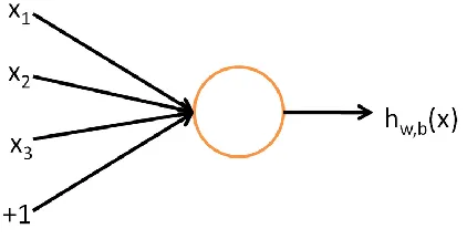
Figure 1: A single neuron with 3 input values, a bias term, and 1 output hypothesis value

(Ng, Ngiam, Foo, Mai, & Suen, 2013) ... 3

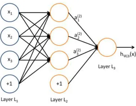
Figure 2: A neural network organized into 3 layers. L1 represents the input layer, L2 is a

hidden layer, and L3 is the output layer. (Ng, Ngiam, Foo, Mai, & Suen, 2013) ... 4

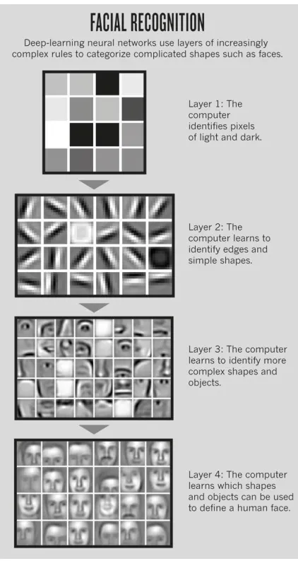
Figure 3: Facial recognition using a deep neural network, demonstrating the multiple levels

of abstraction of the task, from low dimensional pixels to complex shapes and objects

defining a human face. (Jones, 2014) ... 6

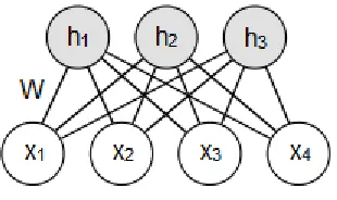
Figure 4: A restricted Boltzmann Machine with weighted connections between a layer of 4

visible input units, x, and a layer of 3 latent hidden units, h. ... 10

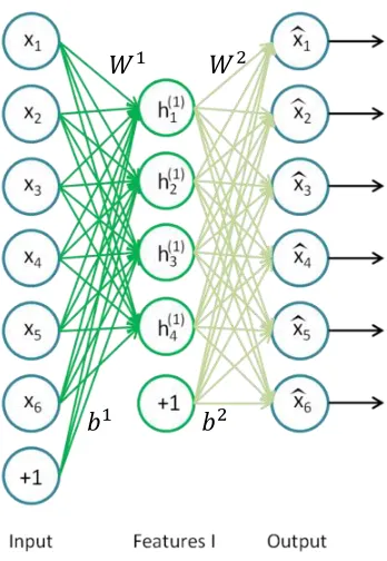
Figure 5: A single layer autoencoder which will be the first in the stack. The weighted

connections from the input layer, , join to the hidden layer, , represented by a matrix, ,

and the weights from the hidden layer, , to the output units, , (the representation of the

input) are stored in the matrix (Ng, Ngiam, Foo, Mai, & Suen, 2013). ... 16

Figure 6: The second autoencoder in the stack. The output from the first autoencoder’s

hidden feature layer (Figure 5) is used as input to the second autoencoder (Ng, Ngiam, Foo,

Mai, & Suen, 2013). ... 17

Figure 7: A 442 442 matrix depicting the global patterns of functional connectivity

among the 442 voxels from the fMRI data. One row of the matrix represents one voxel’s

connectivity with each of the 442 voxels representing in the columns. The closer is to 1

(red/darker), the stronger the association. ... 27

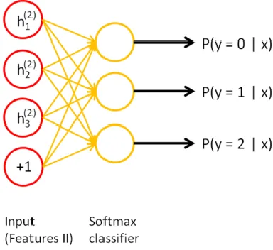
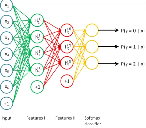
Figure 8: Continuing to build the stacked autoencoder from Figures 5 and 6, the activation

vector resulting from the last hidden layer in the network is used as input to the softmax

classifier which determines the probability of each possible label (Ng, Ngiam, Foo, Mai, &

(9)

viii

capable of classification. The output activations of the second (and final) hidden layer are

input into the softmax classifier (Ng, Ngiam, Foo, Mai, & Suen, 2013). ... 39

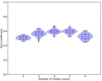
Figure 10: Violin and box plots depicting the distribution of Dice coefficients from

parcellations trained and tested on autoencoders with 2 – 6 hidden layers. ... 46

Figure 11: Each row depicts 3 dimensions of a single parcellation of the medial parietal

cortex: (a) displays the ground truth parcellation verified by anatomists; autoencoders trained

and tested with (b) 3 hidden layers, = 0.638 ± 0.037, (c) 4 hidden layers = 0.676 ±

0.026, (d) 5 hidden layers, = 0.679 ± 0.029. ... 48

Figure 12: Zoomed-in parcellations of the medial parietal cortex where (a) shows the ground

truth parcellation based on expert verified labels of functional regions in 3 dimensions and

(b) shows a parcellation acquired from a deep autoencoder with 5 hidden layers. The spatial

(10)

ix

List of Appendices

Appendix A: Dice coefficients comparing parcellations acquired from autoencoders trained

and tested with 2 hidden layers versus the ground truth parcellation provided by anatomists.

The bolded row represents the parcellation with the maximum accuracy. ... 61

Appendix B: Dice coefficients comparing parcellations acquired from autoencoders trained

Appendix C: Dice coefficients comparing parcellations acquired from autoencoders trained

Appendix D: Dice coefficients comparing parcellations acquired from autoencoders trained

(11)

Chapter 1

1

Introduction and Literature Review

Artificial intelligence has developed significantly in recent years as machine learning and

classification algorithms have become more sophisticated and powerful. Currently, one of

the most popular and promising approaches to machine learning is deep learning (Ng,

Ngiam, Foo, Mai, & Suen, 2013). Deep learning involves learning the hierarchical

structure of data by initially learning simple low-level features which are in turn used to

successively build up more complex representations, capturing the underlying regularities

of the data. Stacked sparse autoencoders are a type of deep network capable of achieving

unsupervised learning – a type of machine learning algorithm which draws inferences

from the input data and does not use labelled training examples. Sections 1.1 – 1.6

discuss the history and theory behind deep learning.

Functional brain parcellation is the task of delineating the brain based on functional

connectivity. This active area of neuroscientific research lacks an ideal standard protocol

as the current techniques assume unrealistic similarity of anatomic composition among

subjects, depend on manual feature engineering, or heavily labelled examples (further

discussed in section 1.7). Therefore, the motivation of this thesis will be to develop a

solution for unsupervised brain parcellation using a deep network to automatically

delineate brain regions based on functional connectivity.

1.1 History of Artificial Neural Networks

Research of artificial neural networks was developed for two distinct areas of study: to

model biological processes in the brain, and to investigate the application of neural

networks to artificial intelligence (AI). While there are parallels between the two

domains, neural networks used in AI are generally simplified models of biological neural

processing and the degree to which artificial neural networks imitate actual brain function

(12)

Artificial neural networks were initially developed by McCulloch and Pitts in 1943. A

neuron is used to represent a computational unit that takes some input values and

produces an output, based on an activation function (McCulloch & Pitts, 1943). For

example, a binary threshold activation function (commonly known as the Heaviside step

function) is an all-or-nothing approach which will result in the neuron “firing”

(outputting results) if the output value is 1, while it will not fire if the output value is 0.

McCulloch and Pitts developed this neural model using electric circuits and proposed that

modelling neurons using this binary threshold activation function mimics first order logic

sentences. That is, providing a neuron with different combinations of 0 (false) and 1

(true) inputs can accurate represent AND, OR, NOT, NAND, and NOR statements at the

output. However, it was later shown that the single model (one neuron) could solve

neither the exclusive-or (XOR) nor exclusive-nor (XNOR) (Minsky & Papert, 1969).

In the late 1940s, Donald Hebb improved the neural network by proposing that neural

pathways are strengthened the more they are used, pointing out that this concept is

fundamental to the process of human learning and memory (Hebb, 1949). Thus,

McCulloch and Pitts's neuron model was altered to account for this learning process. The

solution involved assigning non-identicalweights to each input. Consequently, an input

of 1 may possess more or less weight, relative to the total threshold. Based on these new

developments, Frank Rosenblatt introduced the perceptron, a neural model took input

values ( to ) and corresponding weights ( to ) (Rosenblatt, 1962). Each of the

input values is weighted and summed at the node which only “fires” (outputs) if the

threshold value is reached. While the perceptron model offered hope for artificial neural

networks, it was later shown that the perceptron could not be trained to recognize many

classes of patterns as this single layer network was only capable of learning linearly

separable patterns. Added the fact that XOR and XNOR statements could not be

represented, the 1960s to 1990s saw a drastic decline of the use neural networks for

practical machine learning (Larochelle, Bengio, Louradour, & Lamblin, 2009) as large

single layer neural networks were inefficient and ineffective at learning tasks (Minsky &

(13)

1.2 Modern Artificial Neural Networks

Based on the perceptron, Figure 1 shows the simplest neural network consisting of just a

single neuron (computational unit) that takes input values, , and a bias

intercept term which is a constant term (not included in the input) used to shift the

activation function to the left or right.

Figure 1: A single neuron with 3 input values, a bias term, and 1 output hypothesis value

(Ng, Ngiam, Foo, Mai, & Suen, 2013)

Given an input, , the network outputs a hypothesis ( ) where and are weight

and bias parameters which can be learned from the input data (Ng, Ngiam, Foo, Mai, &

Suen, 2013). Thus, this input data acts as a training set to train the network to learn these

parameters. This neuron’s hypothesized output is defined as

( ) (∑

) Equation 1

where and represent the weight connection and input to the -th of units,

respectively. In addition, is equal to the activation function, , which will

correspond to the sigmoid function used to scale the outputs to a range of [0,1]:

( )

Equation 2

(14)

A more complex neural network is formed by joining many neurons together, so that the

output of one neuron can be the input to any another neuron in the network. These

neurons can be organized into layers, as shown in Figure 2.

Figure 2: A neural network organized into 3 layers. L1 represents the input layer, L2 is a

hidden layer, and L3 is the output layer. (Ng, Ngiam, Foo, Mai, & Suen, 2013)

In Figure 2, the input values are also denoted as neuron-like units. The leftmost layer of

the network is the input layer. The +1 bias unit corresponds to the intercept term. This

network has 3 input units (not counting the bias). The rightmost layer is the output layer

which happens to only have 1 output unit. Meanwhile, the middle layer is referred to as a

hidden layer, as its values are not visible in the input or output data. There are 3 hidden

units in this network. The connections between each unit (excluding the bias units) each

represent a weight connection. A matrix, , can be composed of all the weighted

connections between units of the adjacent layers, and . Therefore the parameters of

the network are ( ) where ( ) ( ) for the 3 layer model. The

output of each unit in layer is represented by an activation vector, , which represents

learned features from that layer, analogous to the hypothesis ( ).

1.3 Deep Learning

When tasked with a problem to solve, humans often decompose the problem into smaller,

(15)

inadvertently exploit intuition and describe concepts in hierarchical ways, based on

multiple levels of abstraction. For example, an individual seeks to identity an image.

Taking the entire image into account, the individual looks specifically at the important

features of the image. The individual sees a human form in the image, notices facial hair,

body structure, and clothing and determines that the image is a man. That is, the

individual has identified the image by breaking it down into smaller features, such as

“has beard”, “has broad shoulders”, “is wearing a suit” and then determined a

classification for the image. The problem is broken down on many levels. Without much

conscious thought, humans look at much smaller features of images, such as lines,

curves, and edges to determine the higher-level features. These numerous highly-varying,

non-linear features organized into layers are what constitute a deep network (Bengio,

Lamblin, Popovici, & Larochelle, 2007).

Deep learning generally refers to learning models which use feature hierarchies with

many layers. Thus, a deep artificial neural network is a multi-layer network composed of

input and output layers, in addition to numerous hidden layers between the input and

output. Those hidden layers are composed of hidden (or “latent”) units that can be used to

describe underlying features of the data. Figure 3 depicts a common facial recognition

task, in which the input layer represents the pixels of the image while the output is the

corresponding identity (or classification) of the face, while the hidden layers can

represent low-level features, such as edges and shapes, to high-level features, such as

“big eyes” or “small nose”. Learning the structure of a deep architecture aims to

automatically discover these abstractions, from the lowest to highest levels. Favourable

learning algorithms would be unsupervised, depending on minimal human effort, while

allowing the network to discover these latent variables on its own, rather than requiring a

pre-defined set of all possible abstractions. The ability to achieve this task while requiring

little human input is particularly important for higher-level abstractions as humans are

often unable to explicitly identify potential hidden, underlying factors of the raw input

(Bengio, 2009). Thus, the power to automatically learn important underlying features

fuels the popularity of deep architectures as the wide applications of deep machine

(16)

Figure 3: Facial recognition using a deep neural network, demonstrating the multiple

levels of abstraction of the task, from low dimensional pixels to complex shapes and

objects defining a human face. (Jones, 2014)

Deep networks were introduced in the 1980s in Fukushima's Neocognitron (Fukushima,

1980) which presented a hierarchical multi-layered neural network used for pattern

recognition, such as the recognition and classification of handwritten characters.

However, early deep multilayer networks were often believed to be too difficult to train

and they were empirically found to be less effective than networks with only one or two

hidden layers (Tesauro, 1992). Consequently, deep learning was not investigated much in

(17)

Sepp Hochreiter’s 1991 thesis identified the issue as “the vanishing gradient problem”

which had led to this major failure of deep artificial neural network (Hochreiter, 1991).

The problem stemmed from the fact that as a layer of neural network eventually learned a

task reasonably well, the learned features were not successfully propagated to successive

layers in the network. The deeper layers did not receive information in order to account

for these new learned features. Backpropagation via gradient descent had become a

crucial step of training deep networks (Werbos, 1974). However, due to the lack of

computing power available at the time, it was thought to be too slow of an algorithm for

practical training of neural networks, resulting in simple methods such as Support Vector

Machines (SVMs) monopolizing the field (Mourão-Miranda, Bokde, Born, Hampel, &

Stetter, 2005). SVMs are sufficient models for basic, linearly separable data, but lacked

the capability of neural networks to learn for complex, non-linear data.

In 1992, Hochreiter’s mentor, Jürgen Schmidhuber, attempted to solve the problem

associated with deep networks by organizing a multi-level deep hierarchy which could be

effectively pre-trained one level at a time via random initialization and unsupervised

learning, followed by a supervised backpropagation pass for fine-tuning (Schmidhuber,

1992). This method allows each level of the hierarchy to learn a compressed

representation of the input observation which is in turn fed into the next level as the

successive input. The “vanishing gradient problem” was solved, but it was not until 2006

that deep learning regained and surpassed its original popularity.

By the mid-1990s to early 2000s, the standard learning strategy for deep neural networks

often involved randomly initializing the weights of the network (pre-training), followed

by backpropagation via gradient descent. However, this method has been empirically

shown to find poor solutions for networks with multiple hidden layers (Larochelle,

Bengio, Louradour, & Lamblin, 2009). The computational power to arrive at satisfactory

results was still out of reach. As a result, shallow architectures continued to be the

predominant structure for machine learning algorithms. These shallow architectures

consist of only two-to-three levels of data-dependent computational elements. For

example, kernel machines, such as Support Vector Machines (SVMs), and single-layer

(18)

However, it has been shown that deep architectures can be significantly more efficient

(sometimes exponentially) than shallow architectures with respect to computational

elements and parameters needed to fully represent some functions (Bengio, Lamblin,

Popovici, & Larochelle, 2007). Shallow architectures are seriously flawed in their

inefficiency regarding the number of computational units (hidden units), and

consequently require a large supply of training examples (Bengio & LeCun, 2007). On

the contrary, the non-linearity of deep architectures allows highly-varying functions to be

represented compactly, requiring fewer parameters (Bengio, Lamblin, Popovici, &

Larochelle, 2007). While it is not the case that deep architectures are always optimal over

shallow architectures (Salakhutdinov & Murray, 2008), complex high-dimensional

problems with sufficient data to capture the complexity are solved more efficiently and

accurately when adopting a deep architecture for learning (Larochelle, Bengio,

Louradour, & Lamblin, 2009; Lee, Laine, & Klein, 2011). Thus, determining efficient

learning algorithms for deep architectures became a popular area of interest in the

machine learning field.

While deep architectures were promising, the issue remained that many negative

experimental results were suggesting that gradient-based training of randomly initialized

supervised deep neural networks easily got stuck in local minima or plateaus (Bengio,

Lamblin, Popovici, & Larochelle, 2007) and that it becomes increasingly difficult to find

a good generalization as the architecture got deeper (more layers) (Larochelle, Bengio,

Louradour, & Lamblin, 2009).

The algorithm popularized by Geoff Hinton in 2006 revolutionized deep learning as it

employs a deep architecture and introduces a fast, greedy learning method used to

construct multilayer directed networks, layer-by-layer (Hinton, Osindero, & Teh, 2006).

As a result, this algorithm offers a solution to the issue of poor optimization which

originally stemmed from random initialization of the network’s parameters. The

algorithm can quickly find a good set of parameters for the network, even in models with

millions of parameters and many hidden layers. The training method also involves a

fine-tuning component which is capable of learning a very successful generative model,

(19)

classification of hand-written digits (Hinton, Osindero, & Teh, 2006). A major

breakthrough of this generative model is that it can easily interpret the distributed

representations in the hidden layers of the deep network.

1.4 Restricted Boltzmann Machines and Deep Belief

Networks

The network used by Hinton is composed of several stacked restricted Boltzmann

machines (RBMs). RBMs (originally named “Harmoniums”) were first introduced in 1986 by Paul Smolensky. A single RBM consists of a layer of unconnected “visible”

input units, , that have undirected, symmetrical connections with another single layer of

hidden units, . The network is fully connected between the two layers, yet no units

within the same layer are connected to one another, forming a bipartite graph

(Smolensky, 1986). Each connection between units of the two layers has an associated

weight that must be learned, represented by a weight matrix, (Figure 4). Data can be

generated from an RBM by initializing a random state in one of the layers and then

performing alternating Gibbs sampling, a Markov Chain Monte Carlo algorithm which

approximates the distribution based solely on previous states. Given the current states of

the units in one layer, all the units of the other layer are then updated simultaneously.

This process is repeated until the entire system is sampling from its equilibrium

distribution (Hinton, Osindero, & Teh, 2006). RBMs are generative models, meaning that

the training period results in a probability distribution of the training data being learned.

When the model is later used for testing, it may encounter new, unfamiliar data, but the

probability distribution can account for these previously unseen occurrences, yielding a

(20)

Figure 4: A restricted Boltzmann Machine with weighted connections between a layer of

4 visible input units, x, and a layer of 3 latent hidden units, h.

Hinton’s proposed learning algorithm acts on several RBMs stacked on top of one

another to form a generative model called a Deep Belief Network (DBN). The leftmost

layers (or “lower layers” in some graphical representations) of the network are able to

extract low-level features from the input, . These lower level features are fed into the

rightmost layers (or “upper” levels) which represent more abstract features and concepts

which can explain the input observation. That is, the model initially learns simple

concepts which it uses to build more abstract, higher-order concepts (Hinton, Osindero,

& Teh, 2006; Larochelle, Bengio, Louradour, & Lamblin, 2009). To achieve this

learning, the algorithm involves greedily pre-training one layer at a time, using

unsupervised learning at each level in order to preserve information from the input,

followed by a supervised fine-tuning pass through the entire network (Bengio, Lamblin,

Popovici, & Larochelle, 2007) Once the stack of RBMs has been learned, the entire

stacked DBN can be viewed as a single probabilistic model.

This algorithm is particularly interesting as it provides a method for high-level

representations to be learned from low-level data, depending mostly on a large supply of

unlabelled input and limited labelled data which is used to slightly fine-tune the model

for the current task. This revolutionary learning algorithm for deep architectures

eliminates the problem caused by random initialization leading to poor optimization

solutions. This greedy layer-wise training strategy is a crucial tool for improved

optimizations as it initializes the weights in a region near a good local minimum

(greedily), resulting in internal representations that are high-level abstractions of the

(21)

The learning strategy is greedy in that optimization occurs by initializing the parameters

of each layer near a good local minimum, independent of the other layers. Adjustments to

the strength each neuron-like unit depends only on the states of the pre-synaptic and

post-synaptic neurons (Hinton, Osindero, & Teh, 2006). The greedy layer-wise algorithm

involves first learning the parameters between the first 2 layers, while assuming all the

other parameters in the remainder of the network are frozen (tied; unchanging). Once the

first set of parametersis learned, the algorithm freezes all layers except the parameters

between the next 2 layers. This process continues until the parameters between every

layer in the network are optimized.

There is no exact solution to the number of hidden layers required to create an optimal

deep network, nor for the number of hidden units per layer. The most common approach

is to validate the model by training and testing on various numbers of hidden layers and

units. The optimal number of hidden layers in the network tends to depend on the nature

of the input data, specifically how it is organized hierarchically in various levels of

abstraction (Heaton, 2008). The decision of units used is crucial to the success of the

model as it greatly influences the outcome. Too few hidden units results in underfitting,

where the model is unable to adequately detect the structure in complex datasets.

Meanwhile, too many hidden units increase the amount of training time and cause

overfitting, where the information contained in the training set is not enough to train all

the neurons (Heaton, 2008). Various pieces of literature provide different “rules of

thumb” regarding the number of hidden units per layer where each layer should have 2/3

the number of input units (Heaton, 2008), between the number of input and output units

(Blum & Rivest, 1992), twice the number of input units (Berry & Linoff, 1997), or 1/30

of the number of training cases (Heaton, 2008). However, there is no generally accepted

support for these suggestions, so validation with test cases is frequently used to crudely

determine the optimal number for the particular dataset.

Deep networks have developed as tools for a wide variety of applications including

classification tasks (Bengio, Lamblin, Popovici, & Larochelle, 2007; Larochelle, Bengio,

Louradour, & Lamblin, 2009), regression (Salakhutdinov & Hinton, 2008),

(22)

Sermanet, Scoffier, Muller, & LeCun, 2008), and natural language processing (Collobert

& J. Weston, 2008).

Thus, the original idea of deep learning was not wrong. The earlier setbacks associated

with deep architectures were results of not using enough data and being limited in

computational power. Previous deep neural networks did not successfully learn because

they were not given enough time. However, pre-training allows the network to build a

model that is likely to succeed (rather than starting from randomly initialized

parameters), resulting in less time required by the network to learn.

1.5 Training a Deep Model

Hinton, et al. (2006) provide an algorithm to pre-train each layer of the DBN using an

unsupervised approach. This greedy layer-wise unsupervised learning algorithm first

involves training the lower layer of the model with an unsupervised learning algorithm

which yields some initial set of parameters for that first layer of the network. That output

from the first layer is a reduced representation of the input. This output then acts as the

input for the following layer which is similarly trained, resulting in initial parameters for

that layer. Again, the output from this second layer is used as the input for the next layer

until the parameters for each layer are initialized. The overall output of the network is

delivered as the final activation vector.

Following this unsupervised pre-training phase of stacked layers, the entire network can

then be fine-tuned in the opposite direction using backpropagation in this supervised

learning phase. Backpropagation works by continually readjusting the weights of the

connections between units of the network. The readjustment maintains the goal of

minimizing the difference between the actual output vector of the network (the network’s

activation) and the desired output vector (the true target value). As the weights are

adjusted, the internal hidden units better represent important features of the task domain

which are not explicitly part of the input or output values. This ability to capture useful

(23)

earlier, simpler techniques such as the perceptron’s convergence procedure (Rumelhart,

Hinton, & Williams, 1986).

1.6 Autoencoders

In artificial neural networks, backpropagation was developed for improved representation

learning. The process of backpropagation involves readjusting the weights, depending the

on the existence of some expected output. In the 1980s, autoencoders (also called “auto-associators”) were introduced in order to perform backpropagation without a teacher

(Bourlard & Kamp, 1988). That is, autoencoders offer a method of automatically learning

features from unlabelled data, allowing for unsupervised learning.

An autoencoder is an artificial neural network that is able to be trained in a fully

unsupervised way. In previous neural networks, labelled data were required to act as

training examples essential to the backpropagation fine-tuning pass as those labels were

used to readjust the parameters. However, autoencoders provide the opportunity to learn

without this dependence on labelled data. An autoencoder neural network performs

backpropagation by setting the target output values equal to the input values, and thus the

autoencoder is trained to minimize the discrepancy between the data and its

reconstruction (that is, the difference between the actual output vector and the expected

output vector where that expected output is the same as the input vector). As a result,

autoencoders are able to learn without a teacher.

An autoencoder consists of three or more layers: an input layer; some number of hidden

layers which forms the encoding; and an output layer whose units correspond to the input

layer. Hinton et al. defined an autoencoder as a nonlinear generalization of principal

components analysis (PCA) which uses an adaptive, multilayer “encoder” network to

transform the high-dimensional input data into a low-dimensional code, while a similar

“decoder” network is able to recover the data from the code (Hinton & Salakhutdinov,

2006). That is, an autoencoder network with the same number of hidden units as input

(24)

Since the outputs of the network are equal to the input, the autoencoder’s goal is to learn

an approximation of the identity function (Ng, Ngiam, Foo, Mai, & Suen, 2013). While

this may seem like a trivial learning task, placing constraints on the network can reveal

interesting structure of the data. An example of a constraint on the network is a limitation

to the number of hidden units in the hidden layer, thus forcing the network to learn a

compressed representation of the input. This method allows for the discovery of internal

representations of the data that rely on fewer intermediate features. For example, for a

facial recognition task, each pixel of the image may be represented at the input layer.

That data is compressed in the hidden layer into features such as “small mouth” or “wide eyes.” That is, the input data of the face can be described using less data than is actually

given in the image. That compressed data can then be uncompressed in order to

re-represent the input data at the output layer, allowing the facial image to be reconstructed

entirely from the learned features.

Rather than limiting the number of hidden units, an alternative constraint to the network

could be the sparsity of hidden units that are activated. Sparsity is a useful constraint

when the number of hidden units is large (even larger than the number of input values)

that can allow for the discovery of interesting structure of the data (Ng, Ngiam, Foo, Mai,

& Suen, 2013). A sparse autoencoder has very few neurons that are active. A neuron in

an artificial neural network is informally considered “active” (or “firing”) if its output

value is close to 1, while it is considered “inactive” if its output value is close to 0. The

concept of creating a sparse autoencoder involves constraining the neurons to be inactive

most of the time (Ng, Ngiam, Foo, Mai, & Suen, 2013). As a result, even with many

hidden units, the data is constrained, forcing the network to learn the important features

of the data in order to reconstruct it.

With deep architectures, learning-feature hierarchies are formed when lower-level

features are learned and used to compose higher levels of the hierarchy. Similar to how

RBMs are stacked to form DBNs, this deep approach can be extended to non-linear

autoencoders to form a stacked autoencoder network (Bengio, Lamblin, Popovici, &

Larochelle, 2007; Larochelle, Bengio, Louradour, & Lamblin, 2009). A stacked sparse

(25)

which the outputs of each layer is fed into the inputs of the successive layer (Ng, Ngiam,

Foo, Mai, & Suen, 2013). However, optimizing the weights of autoencoders is a

challenging task. Large initial weights cause autoencoders to find poor local minima,

while small initial weights result in tiny gradients in the early layers, proving it infeasible

to train many-layered autoencoders in this condition (Hinton & Salakhutdinov, 2006).

However, if the initial weights are already close to a good solution, optimization

techniques, such as gradient descent, work well. It follows that employing a similar

“greedy layer-wise” learning algorithm (which was used for DBNs) to stacked

autoencoders is an effective method of pre-training the network of a deep autoencoder

(Hinton & Salakhutdinov, 2006).

To see the structural composition of this stacked autoencoder, first consider the single

layer autoencoder network in Figure 5. Let represents the weighted connection

between the unit of layer , and unit of layer , while is the bias associated with

unit i in the layer . These values ( ) are organized in the matrices for each

unit and layer of the network. Considering a single independent layer model (i.e.: a single

autoencoder of the stack, composed of an input, output, and hidden layer), the matrix

is composed of the weighted connection between the input data and the hidden units,

while contains the weighted connection between the hidden units and the output.

Similarly, represents the biases from the bias unit in the input layer to each hidden

unit, while represents the bias from the bias unit in the hidden layer to the output

layer. That is, each single layer module has a set of parameters ( )

representing the weights and biases from the input units to the hidden units, and from the

(26)

Figure 5: A single layer autoencoder which will be the first in the stack. The weighted

connections from the input layer, , join to the hidden layer, , represented by a matrix,

, and the weights from the hidden layer, , to the output units, ̂, (the representation

of the input) are stored in the matrix (Ng, Ngiam, Foo, Mai, & Suen, 2013).

Note that the output units of the single autoencoder in Figure 5 will not actually present

in the stacked autoencoder. They are simply used for the training of the single layer.

Rather, the activation vector which represents the features detected from the hidden layer

are used as input to the following autoencoder which is added to the stack, as seen in

Figure 6. That is, the hidden units of the first autoencoder can be considered the visible

input units to the next autoencoder. As expected, the output units of the second

autoencoder in the stack are a representation of the hidden units of the first autoencoder

(i.e.: the current autoencoder’s input units). Recalling that each single autoencoder has a

set of parameters ( ) representing the weights and biases from the

input units to the hidden units, and from the hidden units to the output units, let

_{represent the parameters} _{for the} _{-th autoencoder.}

𝑊 𝑊

𝑏 𝑏

𝑊 𝑊

(27)

Figure 6: The second autoencoder in the stack. The output from the first autoencoder’s

hidden feature layer (Figure 5) is used as input to the second autoencoder (Ng, Ngiam,

Foo, Mai, & Suen, 2013).

To perform this greedy layer-wise pre-training, consider a stacked autoencoder composed

to layers. The stacked autoencoder can be greedily pre-trained in order to initialize the

parameters of this deep network, in a similar way as the DBN was trained: train the first

layer using the raw input to obtain parameters for the first

autoencoder in the stack, while the rest of the parameters in the remainder of the network

remain fixed. With these initialized parameters, the raw input can be transformed into a

vector, , consisting of the activations (learned features) of the hidden units. The

autoencoder is able to map the input directly to the hidden layer using a parameterized

closed-form equation called an encoder (Ng, Ngiam, Foo, Mai, & Suen, 2013): Noting

that represents the initial input to the network, x, the activation vector of a layer, l, is

given as

( ) Equation 3

𝑊 _𝑊

(28)

where ( )is the sigmoid function, while the step is run forward to acquire the following

variable such that

_{Equation 4}

In other words, denotes the total input to the layer , including the bias, which is

calculated based on the previous activation vector. This encoding step is thus able to

transform the high-dimensional input data into a lower-dimensional code.

The decoding steps are similarly used to map from these learned features from the hidden

space back to the reconstruction of that input. The decoder is a parameterized

closed-form equation used to “undo” the encoding function where

₍ ₎ _{Equation 5}

_{Equation 6}

Thus the decoder recovers the high-dimensional data from the code in order to create the

reconstruction of the input (Ng, Ngiam, Foo, Mai, & Suen, 2013).

This output activation vector, , can then be used as input to train the second layer,

yielding the parameters , and thus a new set of features given by the

activation vector is provided. This procedure is repeated for all subsequent layers of the

network, as the output of each new layer serves as input into the next layer, while the

remaining layers are frozen. Finally, the output activation vector from the final layer

gives the activation of the deepest layer of hidden units which, for the autoencoder, is

the reconstruction of the input vector.

1.7 Brain Parcellation

While the fixed anatomical structure of the brain has been thoroughly studied and

documented, the functional connectivity of the brain is a dynamic, elusive, and

(29)

with well-defined functions, the brain's static structural networks gives rise to dynamic

functional connectivity which performs a vast array of tasks, facilitating perception,

cognition, and actions (Park & Friston, 2013). The mapping of functional connectivity

through the analysis of resting-state fMRI was first demonstrated in 1995 (Biswal, Zerrin

Yetkin, Haughton, & Hyde, 1995), leading neuroscientists to examine the relationship

between resting-state connectivity and the functional organization of the brain, associated

with processes such as language, motor skills, and memory. To better understand how

such diverse, complex function can arise from the brain's static neuronal architecture,

researchers aim to accurately parcellate individual brains based on its functional

connectivity.

Brain parcellation refers to the delineation of structural and functional regions of the

brain (Lee, Laine, & Klein, 2011). It is an important and challenging task to establish

these correspondences across structural and functional brain images. The ability to parcel

out functional brain regions non-invasively would enhance the quality of various

experimental investigations, leading to more accurate across-subject comparisons of

independent functional regions (Cohen, et al., 2008). Successful brain parcellation

provides great benefits to clinical neuroscience and cognitive psychology as the relations

between structure and function become better defined.

Parcellation can be performed by analyzing functional images of the brain. Functional

neuroimaging allows researchers to study the brain's dynamic functional relationships in

real-time, based on the current state of the brain's activity, rather than simply the fixed

anatomical structure of the brain. Current modes of acquiring functional neuroimaging

include fMRI, PET (invasive), fNIRS, EEG and MEG (poor spatial resolution).

Functional magnetic resonance imaging (fMRI) permits researchers to associate

functional activity with specific neuroanatomical regions of the brain with a high degree

of spatial resolution. This non-invasive tool detects changes in blood oxygenation levels

and changes in blood flow resulting from neural activity. When a brain region is more

active, it consumes more oxygen, resulting in increased blood flow to the active area

(30)

a particular mental process. The 3-dimensional brain image is composed of units called

voxels, each representing a cube of brain tissue. A voxel is a 3-dimensional building

block of a 3-dimensional fMRI volume, analogous to a pixel being a 2-dimensional

building block of a 2-dimensional image on a screen. Advances in fMRI analysis have

led to the discovery of biomarkers and diagnostic indicators for a variety of psychological

and neurodegenerative disorders (Henley, Bates, & Tabriz, 2005). The ability to

accurately label various brain regions based on function is imperative to understanding

the relationships between brain function and structural appearance. A full understanding

of these correspondences can be applied to understanding the underlying causes of

various metabolic diseases and fine-scale lesions in the brain, potentially leading to major

advancements in treating and curing diseases such as Alzheimer's disease (Henley, Bates,

& Tabriz, 2005).

Many experiments have been developed which use functional neuroimaging to identify

brain regions associated with various cognitive processes. Oftentimes, these

investigations study which brain areas are activated while some task is being performed

(relative to other tasks). However, these experiments are based on a priori hypotheses

since those experiments are designed for the purpose of acquiring this knowledge

(Mourão-Miranda, Bokde, Born, Hampel, & Stetter, 2005). Ideally, a natural, a posteriori

method of searching for functional localization can be developed and implemented for

general use.

There currently exists no standard protocol for such parcellation of the brain into discrete

regions (Bohland, Bokil, Allen, & Mitra, 2009). A variety of software parcellation

packages are available, many of which depend on a labelled brain atlas which associate

physical structure with function. However, each atlas is often developed using a

parcellation protocol which has only been applied to a single individual or it is simply an

amalgamation of various brains (Lee, Laine, & Klein, 2011), thus these software

packages are often inconsistent as they offer different descriptions of neuroanatomical

organization. An alternate approach to parcellation involves researchers co-registering

brain images to each other, using a template or labelled brain atlas of the same imaging

(31)

anatomical similarly which is often not the case (Lee, Laine, & Klein, 2011). Recent

large-scale efforts have been established to manually apply standard brain parcellation

techniques to many different brain images (www.braincolor.org/protocols), but manual

parcellation is tedious, time-consuming, and heavily dependent on expertise the area

(Lee, Laine, & Klein, 2011). Automatic brain parcellation is a significantly more

reasonable approach than manual, yet the intrinsic variability of the human brain makes

the task of defining consistent correspondences across brains a challenging one for both

humans and computers (Lee, Laine, & Klein, 2011).

The ability to parcellate functional regions of the brain without relying on standard

mappings allows for subject-specific parcellation, providing better diagnoses and

understanding of unhealthy or abnormal brains. For example, stroke patients suffer

permanent damage resulting in lesions in the brain and they subsequently lose the ability

to perform corresponding functions which were originally attributed to the now-damaged

area. However, some patients are able to recover the lost function over months or years.

While the irreversible damage is still present, this re-learning of the function indicates

that another area of the brain has learned to compensate and provide the functionally lost

(Schmah, Hinton, Zemel, Small, & Strother, 2008). Therefore, a subject-specific

functional parcellation technique which relies only on the functional connectivity (and

not anatomic structure) would allow specialists to see the area of the brain providing the

recovering function.

To help alleviate the challenges stemming from subject specific parcellations, automated

parcellation schemes have been developed which do not depend on the use of a brain

atlas. Automatic learning techniques such as Support Vector Machines

(Mourão-Miranda, Bokde, Born, Hampel, & Stetter, 2005), Principal Component Analysis (Zhong,

Wang, Lu, Zhang, Jiao, & Liu, 2009), independent component analysis (McKeown &

Sejnowski, 1998) or single-layer neural networks are used to learn the appropriate

neuroanatomical categorization of fMRI image data. However, a major drawback of

current automatic brain parcellation strategies is that they typically depend on algorithms

(32)

learning complex high-dimensional features (Bengio & LeCun, 2007). In addition, these

techniques heavily rely on labelled training examples data for supervised learning.

Data-driven clustering algorithms offer another approach to partition the brain into

distinct functional regions. Kelly et al. (2012) present a voxel-wise classification of brain

imaging data into natural subsets (clusters) based on intrinsic functional connectivity

using clustering algorithms. The algorithm used assigns each unit of data (each voxel) to

the same cluster, given that the voxel is more similar to voxels assigned to that particular

cluster than any other cluster (Kelly, et al., 2012). The similarity between all pairs of

voxels of intrinsic functional connectivity patterns used for this partition can be

quantified using . The metric is used to measure effect size, which represents the

strength of the relationship between two variables. When used to evaluate the similarity

(as a ratio of variance) of each voxel against every other voxel, the value for each pair

ranges between 0 (no agreement) and 1 (identical). Cohen et al. (2008) introduced the

statistic for the purpose of delineation based on functional connectivity, suggesting that it

provides a better measure of similarity between two images than spatial correlation

because it accounts for differences in scaling and offset between images, while

correlation does not take these factors into account (Cohen, et al., 2008). The matrix

can be calculated as

∑_∑ ( ) ( )

( ) ( )

Equation 7

where and are the values of the voxel at location in the maps and (i.e.: a

correlation matrix), is the mean value of and (i.e.: ( ) ), and is the

grand total mean of across all voxels. The k-means clustering algorithm uses this

statistic to measure similarity in order to partition each voxel into a cluster which

represents a functional brain region. The algorithm was used to delineate the functional

areas of the brain's insula – a component of the brain used for tasks including sensory,

(33)

Most current automatic partitioning techniques continue to depend on heuristic manual

feature engineering (Lee, Laine, & Klein, 2011) which is costly, error-prone, and

impractically dependent on human expertise in the problem domain, thus compromising

the generalizability of the model. For example, while k-means clustering is relatively

effective approach to partitioning, it depends on human expertise and interpretation of the

problem domain in order to select a k-value to represent the number of clusters a priori.

K-means clustering discriminates and is biased towards the training data set. For

example, consider a k-means algorithm set to organize the data into 5 clusters. If an input

that should (ideally) be partitioned into some 6th cluster is encountered, it will be

classified incorrectly. K-means clustering can be biased in this way and it often does not

generalize well, especially for more complex data sets. Additionally, k-means clustering

is very sensitive to initial conditions, thus with different starting conditions, the same

k-means algorithm may result in different partitions of the same data set. Furthermore,

while deep learning can be regarded as high-level feature-extraction, k-means clusters

can be a feature-extractor as well. However, k-means is conceptually equivalent to a

single layer of a deep network and thus suffers the disadvantages associated with shallow

architectures.

In general, the drawbacks of current automated brain parcellation are that they 1) employ

algorithms with shallow architectures, 2) they are based on heuristic manual feature

engineering, or 3) they assume the validity of the underlying feature model (Lee, Laine,

& Klein, 2011). Lee et al. (2011) have attempted to account for these shortcomings by

approaching the task of brain parcellation via deep learning. Specifically, convolutional

deep neural networks are used: Training of the deep network is initiated by performing a

forward propagation pass. Two-dimensional fMRI images were broken up into 28 by 28

image sites where context-aware feature learning is used to obtain the parcellation labels

with the greatest probability, composing the convolutional layers of the network. The

output of these convolutional layers are fed into simple subsampling (pooling) layers in

order to reduce the computational expense of the model, while introducing scale

invariance of the learned features. The output nodes of the network are then compared

(34)

through the network to iteratively fine-tune the parameters. The parcellation is validated

by the Dice coefficient, , which is used to measure the agreement between the expected

output (provided by experts) and the learned brain parcels. The score ranges from 0 to 1

where 1 indicates a perfect agreement. In general, was low for small brain parcels

when compared to larger brain structures, indicating less accurate parcellation of finer

functional areas. The low parcellation performance and the high inter-subject variability

were attributed to the limited training set used for the study (Lee, Laine, & Klein, 2011).

Regardless, the architecture, learning process, and consequent results indicate that deep

learning is a viable tool for successful two-dimensional brain parcellation.

The method presented in Chapter 2 proposes a promising approach for automated

voxel-wise brain parcellation using stacked sparse autoencoders for unsupervised learning of

three-dimensional fMRI data. Semi-supervised softmax regression will be used for voxel

classification based on ground-truth labels of brain regions. This technique is

implemented under the hypothesis that the patterns of connectivity underlying the fMRI

data are of high dimension with features organized complexly in multiple levels of

abstraction which can be extracted most effectively by a nonlinear deep autoencoder. The

implementation details and parcellation results will be presented in Chapter 3, while

Chapter 4 will serve as a final discussion and conclusion of the thesis’s findings,

(35)

Chapter 2

2

Methodology

The design and methodology of developing the presented solution to automated brain

parcellation via deep learning will be outlined in this chapter. Beginning with raw

resting-state fMRI data, a sparse deep autoencoder will be implemented in the Python

programming language, learning to classify neural voxels based only on their functional

connectivity with one another, without regard for their anatomic relations. A general

summary of the algorithm for brain parcellation is outlined in the following 6 steps which

will be further investigated in this chapter: 2.1) Prepare the data, 2.2) Pre-train the

autoencoder, 2.3) Train the softmax classifier, 2.4) Fine-tune the entire network, 2.5)

Parcellate new data, and 2.6) Visualize the parcellation.

2.1 Prepare the Data

The fMRI data of 10 different subjects were used for the training of the autoencoder. The

size of this dataset allows for feasible runtime, but further investigation of this approach

would benefit from a larger sample size. For each subject, the raw preprocessed data is

first loaded into a xifti file format – a format developed for storing neuroimaging data

with metadata for use with Python and C programs. The subject's functional and

anatomical brain images are also loaded into the program to provide reference for the

xifti file. From that file, a correlation matrix is produced using Python’s NumPy library,

associating the time course of each brain voxel against every other voxel. Thus a single

row represents the similarity between a single voxel and every other voxel. Consider the

case with voxels, . An matrix can be formed, composed of Pearson

product-moment correlation coefficients, , such that the coefficient of is at position

in the matrix. The coefficient is defined as the covariance of two variables (i.e.:

), divided by the product of their standard deviations. That is,

(36)

where is the covariance, is the standard deviation of , is the mean of , and

is the expectation (the expected outcome given the probability of each potential

outcome). The coefficients range from [-1,1] such that 0 indicates no correlation, 1

indicates perfect positive correlation, and -1 indicates negative correlation between the

voxels. The matrix is symmetric since the correlation between voxels equals the

correlation between voxels . Additionally, the diagonal of the matrix is always 1

since there is perfect correlation between a voxel’s time-series and itself.

From a row-wise comparison of the matrix, similarities among rows indicate stronger

global associations of connectivity. To measure these associations, this correlation matrix

of voxels will be converted to an matrix, as seen in Figure 7. (Note that “ ”

is the alphabetical character referring to the number of voxels, while “ ” is the Greek character “eta” described as follows) while The statistic (Equation 4) describes the

strength of the similarity between the voxels, as it represents the ratio of variance

between each voxel and all the other voxels. Like the correlation matrix, the matrix

will be symmetric where a single row represents the strength of the connectivity between

(37)

Figure 7: A 442 442 matrix depicting the global patterns of functional connectivity

among the 442 voxels from the fMRI data. One row of the matrix represents one voxel’s

connectivity with each of the 442 voxels representing in the columns. The closer is to

1 (red/darker), the stronger the association.

Using such a matrix allows for the analysis of global correlation patterns among voxels.

Rather than just investigating the interaction between each two voxels, the matrix allows

for the investigation of how each voxel relates to the rest of the voxels as a whole.

Therefore, it is the entire normalized matrix that serves as the initial low-level features

of input fed into the stacked autoencoder. Each row of the matrix is a vector acting as a

single input (visible) unit into the network from which the inherent latent factors will be

extracted, activating the hidden layers of the network.

The whole brain can be investigated using the data or, if a particular area is of interest, a

mask can be applied to the data, allowing the learning procedure to only act on that

brain area. While less information is learned if an area is masked out, the problem

becomes much smaller and easier to manage, resulting in a faster runtime. For this

reason, this thesis will be focusing on the functional connectivity of the medial parietal

(38)

relationship between the sensory and motor systems for tasks such as hand-eye

coordination. Therefore, only the data associated with this region is considered as the

remainder of the data is masked out and ignored.

Once the fMRI data is in the suitable form of input data (a normalized matrix), the

deep sparse autoencoder and softmax classifier will be trained and used for parcellation

of the brain region’s voxels. The final program is dynamic, allowing the user to input

new fMRI data while specifying the desired number of hidden layers and hidden units per

layer in the autoencoder. The remainder of this chapter outlines the procedure followed to

achieve this goal.

2.2 Pre-train the autoencoder

Previous deep learning approaches used random initialization of parameters before

training a network. This was a major downfall of previous deep neural networks as a vast

amount of time was required for the networks to learn, making the technique infeasible

for practical learning. However, Hinton's more recent method involved greedy layer-wise

pre-training of each layer by initializing the parameters near a local minimum (Hinton &

Salakhutdinov, Reducing the dimensionality of data with neural networks, 2006). By

pre-training each layer, less time is required to learn the optimal parameters and the model

becomes significantly more computationally powerful. Recall that with a stacked

autoencoder, each subset of adjacent layers can be viewed as a single-layer autoencoder.

Therefore the output activation vector from the first autoencoder in the stack is then used

as input to the second autoencoder in the stack. Pre-training involves setting the

parameters between adjacent single-layer autoencoders independent of the other

autoencoders in the network. As one set of parameters is being determined (e.g.: the

parameters between layers 1 and 2), the remaining parameters of the network (between

layers 2 and 3, layers 3 and 4, etc.) remained fixed. Recall that the parameters of the

network are ( ) where and are matrices representing the weighted connections

(39)

The following process outlines the method for pre-training each set of parameters

between layers of the network, while also computing the activation features extracted

from each unit of that hidden layer. This activation vector output of each layer is in turn

used as input for the pre-training of the following layer in the stacked autoencoder. This

process demonstrates that the greedy layer-wise pre-training makes use of the same

algorithm applied multiple times, once to each layer of the network, until the entire

network has been pre-trained with optimized parameters.

Given a network of layers, the pre-training will be performed on each layer

independently. Thus, for each layer, , in the network:

2.2.1) Initialize the parameters ( ) to small near-zero values

2.2.2) Optimize the parameters by minimizing the cost function, ( )

2.2.3) Calculate the output activation vector, , and set it as the input for layer

. If (i.e.: the last layer), , is stored for input to the softmax model

The following subsections elaborate of these pre-training steps for a single layer of the

autoencoder.

2.2.1 Initialize parameters

The goal of the pre-training is to minimize the cost, ( ), as a function of and

in order to set the parameters in a good neighbourhood for further training. In order to

do so, these parameters at each layer must be initialized to some small, random, near-zero

value. It is crucial that these parameters are not simply originating at values of 0 as such

an initialization would result in all the hidden layer units learning the same function of

the input (Ng, Ngiam, Foo, Mai, & Suen, 2013).

2.2.2 Optimize parameters

2.2.2.1 Optimization Method

The cost function is minimized using the Limited memory BFGS (L-BFGS) optimization

algorithm provided in SciPy's optimization package. BFGS is a quasi-Newton

(40)

derivatives of the function, as well as the inverse Hessian matrix (matrix of second order

partial derivatives) – a large, costly, and complex factor to store and compute, making it

infeasible for large optimization tasks. However, quasi-Newton techniques overcome this

obstacle by instead using an approximation of the inverse Hessian matrix, which the

method can extract from the first partial derivatives. Regardless, even the quasi-Newton

BFGS method’s approximation of dense inverse Hessian requires significant memory

resources. Therefore, the Limited memory BFGS method offers a solution to this

limitation by only using minimal vectors to represent the matrix implicitly, rather than

fully calculating and storing the full inverse Hessian in memory (Galen & Jianfeng,

2007).

Stochastic gradient descent (SGD) is a simple alternative optimization technique

commonly used in training. However, it not only requires addition fine-tuning of

parameters (a learning rate), but it has been shown to be outperformed by L-BFGS when

training large datasets. In particular, when comparing the two approaches for sparse

autoencoder optimization, L-BFGS has demonstrated faster and more stable training (Le,

Ngiam, Coates, Lahiri, Prochnow, & Ng, 2011). L-BFGS is a sophisticated, yet

easy-to-use off-the-shelf optimization method that offers fast, reliable results, while requiring

only the function to optimize and its gradient. For these reasons, L-BFGS is used

throughout the project for optimization.

2.2.2.2 Cost Function

Starting with randomly assigned, near-zero values for the parameters, pre-training is done

by training each layer individually. Thus as the first layer is pre-trained to find some

optimal parameters, the remaining layers remain fixed. The input data of the entire model

is used as the input data to the first layer. This data is used to determine the parameters

which minimize the cost function of the sparse autoencoder, ( ), and the

corresponding derivatives of ( ) with respect to the parameters ( ).

The ( ) cost function is the sum of three components: a) the average

sum-of-squares error term, b) the weight decay term, and c) the sparsity penalty. The following

Deep Learning via Stacked Sparse Autoencoders for Automated Voxel-Wise Brain Parcellation Based on Functional Connectivity

Scholarship@Western

Scholarship@Western

Deep Learning via Stacked Sparse Autoencoders for Automated

Deep Learning via Stacked Sparse Autoencoders for Automated

Voxel-Wise Brain Parcellation Based on Functional Connectivity

Voxel-Wise Brain Parcellation Based on Functional Connectivity

Abstract

Keywords

Acknowledgments

Table of Contents

List of Tables

List of Figures

List of Appendices

Chapter 1

1

Introduction and Literature Review

1.1

History of Artificial Neural Networks

1.2

Modern Artificial Neural Networks

1.3

Deep Learning

1.4

Restricted Boltzmann Machines and Deep Belief

Networks

1.5

Training a Deep Model

1.6

Autoencoders

1.7

Brain Parcellation

Chapter 2

2

Methodology

2.1

Prepare the Data

2.2

Pre-train the autoencoder

2.2.1

Initialize parameters

2.2.2

Optimize parameters

2.2.2.1

Optimization Method

2.2.2.2

Cost Function