Continuous Flow Processing of Foods using Cylindrical Applicator Microwave Systems Operating at 915 MHZ

ABSTRACT

CORONEL, PABLO. Continuous flow processing of foods using cylindrical applicator microwave systems operating at 915 MHz. (under the direction of Dr. K.P. Sandeep)

Microwave heating of foods is a proven and mature technology for household applications. However, industrial applications of microwave heating of food and

biomaterials are scarce, due to the lack of suitable equipment and research on the subject. Aseptic processing and packaging of foods offers products of high quality with long shelf life. Aseptic processing of low thermal diffusivity and high viscosity food and bio

products can lead to diminishing the quality of such products due to long exposures to high temperatures.

Industrial Microwave Systems (Morrisville, NC) invented a system that allows continuous flow microwave heating of foods in industrial scale, by focusing the

microwave energy in a specially designed cavity. Food products can be pumped through a microwave transparent tube located in the focused area of the cavity and be heated with short time exposure to the microwave energy. Cooperation between Industrial

Microwave System and North Carolina State University started this research.

determine the temperature profile within a cross sectional area of the tube; a method to predict feasibility of a product to be processed by measuring its dielectric properties; and testing sequence to scale-up from bench-top to industrial scale operation were defined.

CONTINUOUS FLOW PROCESSING OF FOODS USING CYLINDRICAL APPLICATOR MICROWAVE SYSTEMS OPERATING AT 915 MHZ

by

PABLO CORONEL

A dissertation submitted to the Graduate Faculty of North Carolina State University

in partial fulfillment of the requirements for the Degree of

Doctor of Philosophy

FOOD SCIENCE

Raleigh 2005

APPROVED BY:

BIOGRAPHY

Pablo Coronel is the eldest son of Marcelo and Catalina Coronel, born and raised in Quito, Ecuador. Thanks to the rigorous and open education provided by his parents, he learned that science is the path to finding the most beautiful things in the universe. Pablo received his diploma in Chemical Engineering from the Escuela Politecnica Nacional, Quito, Ecuador, where he worked under the supervision of Prof. Bolivar Izurieta, and worked on a thesis in the field of Biotechnology with applications to the food industry.

After graduating from the university, he was hired by Sumitomo Corporation to work in the chemical products department, and then by Panificadora Moderna, the largest fresh bread bakery of Ecuador, as production engineer in the main plant, and took charge of the research & development department. He successfully graduated from the science and technology of baking courses, offered by the AIB in 1999. He was part of the team that designed a new plant for the production of extruded baby food based on soybean and cereals that is a part of the United Nations mother and infant feeding program (PANN 2000). The plant opened in June 2000.

Pablo was awarded a Fulbright Scholarship in 1999, which allowed him to pursue a Masters degree in Food Science at North Carolina State University. Under the supervision of Dr. K.P. Sandeep he graduated in December 2001.

ACKNOWLEDGEMENTS

Thanks are dedicated to my parents, Marcelo and Catalina for showing me that the universe is full of wonders awaiting to be discovered and opening my eyes to the great universe of science. Everything I accomplish is thanks to the curiosity and discipline my parents taught me.

This work could not have been accomplished without the wise advice of Dr. K.P. Sandeep, my academic advisor. His patience and wisdom helped me to finish this work and made my studies under his supervision enjoyable. His thoughtful scientific insight

encouraged my interest in digging deeper into the knowledge of the basic principles under every aspect of this research.

Thanks to Dr. Josip Simunovic, senior researcher in this project. His friendship, daily encouragement, enthusiasm and knowledge have made me go through unopened doors and achieve what was thought impossible. I’ll always remember his favorite encouragement phrase “It’ll never work”.

The love of my wife Ana Katalina gave me the courage to work endless days and nights in the completion of this dissertation. Without her support and unconditional love, my body and mind couldn't accomplish the task. My wife, and my daughters Rebeca and

Thanks to the agencies and companies that have funded and made this project a reality, Industrial Microwave Systems, Center for Advanced Processing and Packaging Studies, Southeastern Dairy Foods Research Center, and United States Department of Agriculture.

Special thanks to Gary Cartwright and Jack Canady, for their help in the setup and operation of the equipment. No work could have been done without their effort and experience. Thanks to the Personnel of the NCSU Dairy Pilot Plant for their support and help day in and day out.

TABLE OF CONTENTS

List of Tables ... x

List of Figures ... xi

1. Introduction ... 1

2. Literature review ... 3

2.1 Aseptic processing of foods ... 3

2.1.1 Thermal processing of foods ... 3

2.1.1.1 Kinetics of microbial inactivation... 7

2.1.1.1.1 D and z values ... 7

2.1.1.1.2 Thermal destruction time and cook value ... 9

2.1.1.1.3 Considerations for continuous flow processing ... 10

2.1.2 Aseptic processing and packaging ... 12

2.2 Introduction to microwaves ... 16

2.2.1 Electromagnetics ... 16

2.2.1.1 Maxwell’s equations ... 17

2.2.1.2 Poynting vector ... 20

2.2.1.3 Propagation of electromagnetic waves... 21

2.2.1.4 Electromagnetic waves at interfaces ... 26

2.3 Microwave heating of foods ... 29

2.3.2 Applications in food materials ... 31

2.3.3 Components of a microwave heating system... 32

2.3.3.1 Magnetrons ... 32

2.3.3.2 Waveguides... 35

2.3.3.3 Impedance matching ... 43

2.3.3.4 Resonant application cavities ... 44

2.4 Dielectric properties of food materials... 45

2.4.1 Measurement of dielectric properties ... 48

2.4.2 Temperature dependence ... 50

List of symbols ... 54

References ... 58

MANUSCRIPT I Temperature profiles within milk after heating in a continuous flow tubular microwave system operating at 915 MHz Abstract ... 65

Introduction ... 66

Materials and methods ... ... 69

Results and discussion ... ... 73

Conclusions ... 76

Acknowledgements ... 77

References ... 79

MANUSCRIPT II Dielectric properties of selected pumpable food materials at 915 MHz Abstract... 92

Introduction... 93

Materials and methods... 95

Results and discussion... 96

Conclusion ... 101

Acknowledgements ... 102

References... 103

MANUSCRIPT III Preparation of sterilization solutions for aseptic processing of foods in continuous flow microwave systems operating at 915 MHz Abstract... 114

Introduction... 115

Materials and methods... 116

Results and discussion... 117

Conclusion ... 123

References... 124

MANUSCRIPT IV

Aseptic processing of sweetpotato purees using a continuous flow microwave system operating at 915 MHz

Abstract... 136

Introduction... 137

Materials and methods... 138

Results and discussion... 143

Conclusion ... 148

Acknowledgements ... 149

References... 150

Nomenclature ... 152

List of figure legends... 152

MANUSCRIPT V Solution of the Helmholtz equation to determine the feasibility of continuous flow microwave processing of food and biomaterials using tubular applicator systems. Abstract... 162

Introduction... 163

Mathematical background ... 164

Solution of the Helmholtz equation ... 166

Classification of food and biomaterials based on their feasibility to be processed using

continuous flow microwave heating systems ... 171

Conclusions... 173

Nomenclature... 174

References... 175

LIST OF TABLES

LITERATURE REVIEW:

Table 2.2.1 Generalized form of the Maxwell equations ... 18 Table 2.3.1 Current applications of microwave heating in the food industry ... 32 Table 2.3.2 Standardized dimensions for rectangular waveguides for use in microwave

heating ... 42 Table 2.4.1 Methods to measure dielectric properties... 49

MANUSCRIPT I

Table 1: Dielectric properties and penetration depth for milk at 915 MHz ... 81

MANUSCRIPT II

Table 1: Products tested in this study... 105 Table 2: Correlations for dielectric properties as a function of temperature

LIST OF FIGURES LITERATURE REVIEW

Figure 2.2.1: Propagation of electromagnetic waves in a dielectric material... 24

MANUSCRIPT I

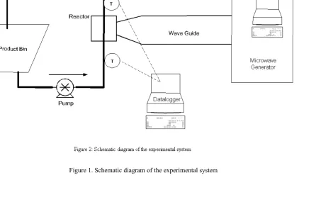
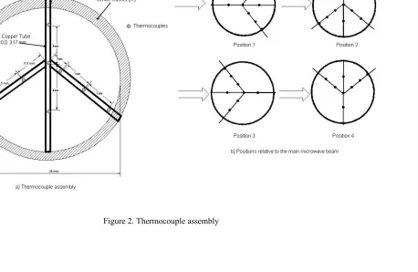
Figure 1: Schematic diagram of the experimental system ... 82 Figure 2: Thermocouple assembly used in this study ... 83 Figure 3: Mean outlet temperature of different types of milk as a function of inlet

temperature ... 84 Figure 4: Mean outlet temperature of skim milk as a function of inlet temperature... 85

Figure 5a: Distribution of temperature increase at the exit of the tube for skim milk at 2.0 l/min ... 86 Figure 5b: Distribution of temperature increase at the exit of the tube for skim milk

at 3.0 l/min ... 87 Figure 6a: Temperature distributions in the cross sectional area at different inlet

temperatures for skim milk at 2.0 l/min ... 88 Figure 6b: Temperature distributions in the cross sectional area at different inlet

MANUSCRIPT II

Figure 1: Dielectric properties of milk and dairy products... 107

Figure 2: Dielectric properties and specific heat of chocolate milk... 108

Figure 3: Dielectric properties of soy beverages ... 109

Figure 4: Dielectric properties of puddings ... 110

Figure 5: Dielectric properties of avocado products ... 111

Figure 6: penetration depth as a function of temperature for representative products from each group ... 112

MANUSCRIPT III Figure 1: Dielectric properties of table salt solutions as a function of concentration and temperature at 915 MHz... 126

Figure 2: Dielectric properties of sugar solutions as a function of concentration and temperature at 915 MHz... 127

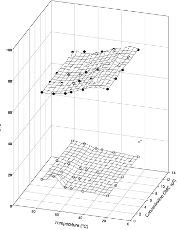
Figure 3: Dielectric properties of CMC solutions as a function of concentration and temperature at 915 MHz... 128

Figure 4: Dielectric constant of salt-sugar mixtures as a function of temperature ... 129

Figure 5: Loss factor of salt-sugar mixtures as a function of temperature... 130

Figure 6: Dielectric properties of CMC-salt mixtures as a function of temperature ... 131

processing of sweet potato puree ... 133 Figure 9: Time-temperature profile during sterilization (using solution #3) and

processing of sweet potato puree ... 134

MANUSCRIPT IV

Figure 1: Schematic diagram of the processing system used in this study... 153 Figure 2: Dielectric properties of SPP at 915 and 2450 MHz ... 154 Figure 3: Maximum operating diameter of SPP at 915 MHz ... 155 Figure 4: Typical temperature profiles at the exit of the heating section

in the 5kW test ... 156 Figure 5: Rheological properties of SPP samples from the 5kW test ... 157 Figure 6: Color measurements of SPP samples from the 5kW test ... 158 Figure 7: Typical temperature profile at the inlet of the holding tube during the 60kW

test before static mixers were used... 159 Figure 8: Typical temperature profile at the inlet of the holding tube during the 60kW

test after static mixers were used ... 160

MANUSCRIPT V

Figure 1: Modes of propagation of electromagnetic waves in cylindrical cavities... 165 Figure 2: Penetration of microwave electrical field in a 38mm ID tube for materials

with different dielectric properties (ε ' = 1 to 100 and ε"= 40) ... 177 Figure 4. Penetration of microwave electric field for 3 materials (a: ε '=40, ε ''=20; b: ε '=40, ε ''=80; c: ε '=60, ε ''=80) in 4 different cylinder diameters

(ID = 10, 38, 60 and 150 mm) ... 178 Figure 5: Penetration of microwave electrical field in a 38mm ID tube for materials

with different dielectric properties

(ε ' = 1 to 100 and tan δ = 0.1, 0.5, 1.0 and 2.0))... 179 Figure 6: Absorption of microwave power in a 38mm ID tube for materials

with different dielectric properties (ε' = 40 and ε "= 1 to 100) ... 180 Figure 7: Absorption of microwave power in a 38mm ID tube for materials

with different dielectric properties (ε ' = 1 to 100 and ε"= 40) ... 181 Figure 4. Absorption of microwave power for 3 materials (a: ε '=40, ε ''=20;

b: ε '=40, ε ''=80; c: ε '=60, ε ''=80) in 4 different cylinder diameters

(ID = 10, 38, 60 and 150 mm) ... 182 Figure 9: Absorption of microwave power in a 38mm ID tube for materials with

different dielectric properties

(ε ' = 1 to 100 and tan δ = 0.1, 0.5, 1.0 and 2.0)) ... 183 Figure 10. Value of the relative absorbed power in the center of the tube as

a function of the dielectric properties of the materials (ε’ and ε”)

for a 39mm ID cylinder ... 184 Figure 11. Calculated temperature increase of product with dielectric properties of milk

1. Introduction

Aseptic processing and packaging of foods provides a method to produce safe and high quality foods. While this method of preservation of foods has been known and applied to some food products, there is still need for improvement in rapid heating and cooling methods to improve the quality of the foods processed this way.

The use of microwaves for thermal treatment of fluid foods is an emerging technology in the food industry. Microwave heating promises rapid heating of food materials, which could be applied in aseptic processing and packaging. Research on this subject is underway in several institutions, but applications are still scarce. The lack of suitable equipment and the economics of the processing have been the main drawbacks of this technology.

Initial research in the use of continuous flow microwave heating was performed using household microwave ovens, through which a small diameter tube was inserted and food was pumped through the tube. These tests however had many drawbacks like the use of a small diameter tube, very small throughput, and the lack of controllability of the microwaves in the heating chamber. Household microwave ovens are designed using a box type heating cavity which adds complexity to the analysis of the electromagnetic distribution and absorption due to the presence of random modes inside the cavity. In order to overcome these problems a focused application cavity was required.

being heated, improving the efficiency of the energy transfer. Cooperation between IMS and North Carolina State University allowed the use of their technology, and resulted in this study.

2. Literature Review

2.1 Aseptic processing of foods

The ultimate goal of food processing is to provide safe foods with long shelf life that have the nutritional and quality attributes preserved as close to those of the fresh food as

possible. Besides the requirement of high quality ingredients, processing has to be carried out in a manner that will preserve the quality attributes of the food materials, while minimizing the risk of microbial contamination. Food preservation processes including fermentation, salting, drying, and thermal processing have been used for many years. Thermal processing possesses a greater importance than the other methods due to the wide acceptance and utilization of this method to preserve foods around the world (Potter and Hotchkiss, 1995).

2.1.1 Thermal processing of foods

Thermal processing of foods is the most common method used to eliminate

microorganisms in order to extend the shelf life of foods and avoid spoilage. Thermal processing relies on the use of heat to cook the food and eliminate microorganisms, and consists of one or a series of heat-hold-cool cycles. The product to be processed can be either packaged like in retort processing, or processed in bulk like in continuous flow processing. In the latter case, a

detrimental to quality, by destroying not only heat-sensitive components but also degrading proteins and producing non-enzymatic browning (Singh and Heldman, 2001).

The equipment used for thermal processing of foods includes retorts, plate-, shell and tube-, and scraped surface- heat exchangers, steam injection and infusion systems. Steam and hot water are the most common heat sources for thermal processing, used directly or indirectly on the food material, with the advantages of being widely available, relatively inexpensive, and well studied. Other alternative heat sources such as microwave, radio frequency, ohmic, and infrared heating are being studied for improved thermal processing of foods (Sing and Heldman, 2001).

There are several levels of thermal processing of foods with pasteurization, and sterilization being the two of the most widely used. Pasteurization refers to a process used to inactivate the microorganisms that may cause a public health concern, and at the same time extend the shelf life of the food products from an enzymatic and microbial point of view. Foods subject to pasteurization still contain microorganisms capable of growing and producing spoilage of foods, and usually require additional preservation processes such as refrigeration to lengthen their shelf life. A classic example of a pasteurized product is milk. Sterilization refers to a process in which the product is rendered free of microorganisms. However, rendering a food product completely free of microorganism is not practical because it would require large amounts of energy, and can result in an unacceptable product. Thus, a more practical level of destruction of microorganisms called commercial sterility has been defined for foods.

Commercially sterile foods are those processed to a degree such that the product is free of

spoilage under non refrigerated conditions. These foods have long shelf life (over 1 year) and can be stored without refrigeration (Potter and Hotchkiss, 1995).

Commercially sterile foods are widely available, in the form of canned foods. These foods are packaged in metallic cans, and after being packaged the cans are heated in autoclaves using steam until the “cold spot” of the can receives the necessary thermal treatment. The location of the cold spot in a can is a critical issue, and depending on the characteristics of the foods it can be located either in the geometrical center of the can if the heat transfer inside the food is mainly by conduction, or at two thirds of the height of the can if the heat transfer inside the food is mainly by convection. The thermo-physical properties of the material, such as thermal conductivity, viscosity, and specific heat will influence the way the heat is transferred within the food product. Stratification of temperature and high temperature differences between locations within the food can be found, which in turn lead to over processing of certain parts of the food, that can cause degradation of the food and render it unacceptable to the consumers. Size of can that can be processed using this method is limited, due to time and energy

consumption considerations (Singh and Heldman, 2001).

Continuous flow processing promises an improvement in quality of the food, and

certain length of tube (holding tube) is used to provide the necessary time for the inactivation of microorganisms. The food product is afterwards cooled and packaged in containers according to the shelf life expected or the customers requirements.

Temperatures used for these processes are higher and holding times are shorter than in canning, rendering a product with higher nutritional and sensorial qualities. Due to the

convective heat transfer mechanisms occurring in these type of processes, the temperatures are more uniform than in canned foods, so the product is processed uniformly. In order to ensure that the food product has been sufficiently processed, the slowest heating point of the product has to be sufficiently processed. In the case of a homogeneous fluid, either in laminar or turbulent flow, the center of the tube is considered to be the critical point. If the food contains particulates, the center of the fastest moving particle and with the poorest thermal properties has to be

considered the critical point. All efforts have to be made to insure that these critical spots have received the correct thermal processing (Sastry and Cornelius, 2002).

2.1.1.1 Kinetics of microbial inactivation

The simplest and oldest way to thermally process foods is by packaging them in a metallic can and then increasing the temperature of the food product inside the can using steam until the number of microorganisms left is consistent with the degree of processing desired. In order to achieve the balance between time and temperature it is necessary to learn how the reduction of the number of microorganisms is achieved.

2.1.1.1.1 D and z values

Initial work on the destruction of microorganisms was carried out by Bigelow, Ball, Esty and others during the early part of the 20th century. Those studies showed that when

microorganisms are subject to constant temperature, the number of surviving microorganisms decreased in a manner that followed first order kinetics, i.e., a straight line in a logarithmic plot. They observed that at constant temperature the decrease of the population (N) was dependent on the initial population (N0), the time of exposure to such temperature (t), and the type of

microorganism, denoted by a constant (k) specific of each microorganism. The kinetics of this destruction could be modeled into an Arrhenius-type model and the equation describing the destruction of microorganisms at constant temperature was written as follows:

t k 0 e

N

N₌ − _[2.1.1]

In order to allow for simpler mathematics, equation 2.1.1 was transformed to allow the use of common logarithms, such that:

D / t 010

N

where D is the time required to decrease the microbial population by 90% or one logarithmic cycle, and is called the decimal reduction time or D value.

D value is a characteristic of the microorganism being studied. Further experiments showed that the D value for a given microorganism was dependent on the temperature at which the process was carried out. By testing the reduction of the same type of microorganism at different temperatures, they observed that the D value followed Arrhenius type kinetics such that:

RT Ea e K

D= − [2.1.3]

where K is a constant and Ea is the activation energy for the destruction kinetics of a given

microorganism. This equation was modified to use common logarithmics and parameters that are simpler to measure, such as D0 at a reference temperature (T0), such that:

z T T 0

0 10 D D

− −

= [2.1.4]

where z is called thermal resistance of the microorganism or z value.

2.1.1.1.2 Thermal death time and cook value

In order to evaluate the efficiency of a method to reduce the population of

microorganisms, the complete thermal treatment must be evaluated and this is accomplished by an integration of the above mentioned parameters. The thermal death time (TDT) or F-value is calculated using the following equation:

dt 10 F t 0 z T ) t ( T 0 0

∫

The subscript "0" is used to denote that the sterilization value has been normalized to a reference microorganism at a reference temperature (T0). This method was proposed initially by Bigelow

and others (1920) and has been used as a conservative approach to processing. The reference temperature used is 121.1 °C and the reference z value is that of Clostridium Botulinum (10 °C) at given reference temperature (Jackson and Lamb, 1981).

The destruction of nutrients, changes in texture, and elimination of enzymes follow similar kinetics to that of the destruction of microorganisms, but it has been proven that the z values for destruction of components of food products have to be reevaluated. Nutrient

destruction in food products is calculated by using the equation introduced by Mansfield (1961), in which the thermal death time has been renamed as Cook value or C0 value, and a redefined zN

value is used, as follows:

dt 10 C t 0 z T ) t ( T 0 N 0

∫

for this value, the common reference parameters are T0 = 100 °C and zN = 33 °C (Jackson and

The TDT method is used in industry, and it reflects a pseudo steady state model, which is based on canned foods in a constant temperature medium (steam), without agitation. However, continuous flow processing is not a steady state process. Therefore, modifications to the above-mentioned method are required in order to estimate the thermal effects in a more realistic manner. The heat-hold-cool cycle to which the products are exposed may last only a few seconds, and the heating and cooling are carried out in unsteady state. Therefore, additional considerations are necessary to estimate the microbial inactivation in these systems.

2.1.1.1.3 Considerations for continuous flow processing

In order to address the unsteady heat transfer, and subsequent thermal processing of food in continuous flow processes, where the changes in temperatures and flow parameters occur at very fast rates, it became necessary to revise the TDT methods. The standard TDT method is a conservative one, in which time and temperature are only taken into consideration in the holding tube, and come up and cool down times are neglected. However, when high temperatures are used, the heating and cooling of the products can have a large influence in the destruction of microorganisms as well as in changes in quality factors.

Swartzel (1982) proposed modifications to the traditional F0 value thermal evaluation

protocol to be suitable for continuous flow processing. A simulation of the processing

equivalent temperature (TE) and time (tE) are calculated to contrast canning to continuous flow

processing, and it was demonstrated that these equivalent values were independent of activation energy, thus being valid for all the inactivation or cooking processes in the system. First, the thermal reduction relationships (G value) are calculated using equation 2.1.7 for each component of the food being tested. Then the equivalent point is found by finding the values of TE and tE

that satisfy equation 2.1.8. TE and tE can be calculated by solving equations 2.1.7 and 2.1.8 for

several activation energies. In other words, if logarithmic plots of the thermal reduction

relationships versus reciprocal temperature are generated for several G-Ea pairs, the lines should

intersect at a point that corresponds to the equivalent point.

dt e G t 0 ) t ( T R Ea

∫

G= − [2.1.8]

Experimental verification of the EPM method showed that finding solutions of equation 2.1.8 was not trivial, and that some of the assumptions of the method had to be revised. The method was based on the existence of a unique intersection point of the different G-Ea curves,

but this was not observed in experiments. Sadeghi and other (1986), Nunes and others (1991), Nunes and others (1993), and Maesmans and others (1994 and 1995) investigated this

isothermal conditions, and Welt and others (1997) further extended the method and called it the Paired Equivalent Isothermal Exposure method (PEIE).

Kyereme and others (1999) investigated a procedure to improve the accuracy of the calculation of the equivalent point. It had been shown that tE depends not only on the activation

energies and G values of the different products, but also on TE,. Thus, multiple intersection

points may exist between different G-Ea lines for different products (1 and 2) as shown in the

equation system 2.1.9.

) G / G ln( R E E T 2 1 1 a 2 a E −

= [2.1.9a]

E 1 a T R E 1 E G e

t = [2.1.9b]

The equivalent F0 and C0 are calculated by plotting the intersection of characteristic

curves. Characteristics curve are defined by plotting the solutions to the system of equations 2.1.9 on a log(tE) - TE plot, which results in a line with slope of -1/z. The tangent line is a plot of

all the equivalent points. This method gives more accurate results and can be used to estimate the sterilization values in continuous flow processing of foods.

In summary, kinetics of microbial and nutrient inactivation are important to achieve safe and high quality products, continuous flow processing is the technology this study has been focused on, and especially aseptic processing.

2.1.2 Aseptic processing and packaging

sterilized and the food product is filled into the package in a sterile environment. This method of processing and packaging provides food with very long shelf life (>2 years).

Aseptic processing of foods takes place at high temperatures and short holding times to assure microbial destruction, while retaining nutrients and sensorial qualities of the products. Typical process temperatures are between 120 and 150 °C with holding times between 5 and 90 s. Population of microorganisms is reduced very fast at high temperatures, and only short times of exposure are required. The undesirable changes in the food materials due to thermal treatment that result in changes in flavor, color, odor, reduction of nutrients, and denaturation of proteins are less likely to occur in the short times to which products are exposed during aseptic processing (Reuter, 1987).

The equipment used for aseptic processing differs in some aspects to the equipment used in other food processing, because of the unique requirements of this kind of processing. Besides of the specially designed packaging equipment, the heating and cooling stages of the processing need to be as short as possible.

The main concern with aseptic processing is to keep all of the components free of microbial contamination; product, processing and filling lines, surge tanks, packaging environment and materials. The system has to be presterilized prior to processing, which is achieved using hot water for the processing and filling lines, saturated steam for the surge tanks and scraped surface heat exchangers, and sterile air for the packaging environment. The

packaging materials are sterilized in line using peroxides, or other chemicals together with sterile air.

The packaging equipment is the most significantly different component of an aseptic process line, when compared to a conventional canning process. The packaging material needs to be sterilized before it is formed, and a stream of sterile air is used to keep the whole

environment microorganism free. Form-fill-seal machinery is preferred, such as carton and plastic, but bag-in-box fillers in which the bags are pre-sterilized using hot steam are used for high capacity filling (Reuter, 1987).

The main advantages of this technology when compared to canning are the possibility of continuous operation, flexibility of packaging options and sizes, smaller foot print, lower cost of packaging and greater quality and sensorial attributes due to the shorter heating time cycles the product is exposed to. The disadvantages include a high expenditure in equipment, the need for trained people, and the lack of mechanical stability that plastic and cardboard packaging posses (Singh and Heldman, 2001; Reuter, 1987).

Homogeneous food products, such as milk, cooking sauces, chicken broth, tomato paste, and fruit juices, are currently being processed using this technology. However, aseptic

FDA, and many concerns include not only the sufficient thermal treatment of the particles but also the possibility of having particles in contact with the seal portion of the packaging, preventing the formation of impervious seals. (Sastry and Cornelius, 2002).

Aseptic processing of foods is carried out in continuous flow and one of the requirements is the rapid heating and cooling of the food materials. Due to the FDA regulation, only the lethality accumulated in the holding tube can be accounted for the requirements of commercial sterility, but the heating and cooling sections may provide a significant lethality as well. This conservative lethality imposed by the law may be detrimental to the quality of the product. The high temperatures used in aseptic processing may destroy the nutrients of the food material to a greater extent than initially intended, if the exposure of the food to such high temperature is underestimated by a few seconds. For this purpose, specialty heat transfer equipment has been designed trying to maximize the heat transfer rates. Both indirect and direct heat exchangers have been improved and worked on. Yet the same limitations given by the thermophysical properties of the food materials are present. Steam infusion and steam injection have been proposed as rapid heating methods, but they have the disadvantage of introducing water into the product, which later needs to be flashed out (Reuter, 1987; Singh and Heldman, 2001).

2.2 Introduction to microwaves

The electromagnetic spectrum includes waves with frequency that range from 300 to 300,000 MHz, corresponding to wavelengths of 0.001 to 1 m. These waves are called

microwaves and are used for radar, telecommunications, television, and heating of food products (Ishii, 1995; Sadiku, 1995).

The use of microwaves to heat food products was discovered by Percy Spencer in 1946, while working on a military radar project for Raytheon corp. Spencer stopped for an instant in front of a microwave generator and noticed that a chocolate bar he had in his pocket had melted. Soon afterwards, Spencer began to experiment with some other food products and noticed that microwaves could be used to heat foods in a rapid and efficient manner. For this invention, Spencer was granted patent number 2,495,429 for a “method of treating foodstuffs” in 1950. Raytheon corp. began the production of commercial microwave ovens in 1947 under the name Radarange, although they were aimed for commercial use being 1.8 m tall and weighing over 300 kg. A smaller microwave oven, for use in homes and offices, was introduced in 1967 by Amana Corp. Since then, the microwave oven has become a ubiquitous appliance in the

American lifestyle. While the microwave oven is a modern appliance, the underlying principles of heating using microwaves were discovered many years before, through the work of many scientists in the field of electromagnetics.

2.2.1 Electromagnetics

quantities of straw, paper or hair by the 6th century B.C., but the knowledge of electromagnetism was stagnant for over two millennia. It was just at the turn of the 18th century that the industrial revolution sparked interest in the field again. The work of James Clerk Maxwell led to several inventions that allowed the practical usage of electromagnetism with the invention of the light bulb, the telegraph, and the telephone by the end of the 19th century. The presence of

electromagnetic waves was acknowledged due to the work of Hertz (1857-1894) and led to the invention of the radio (1899), television (1927), and modern telecommunications. All these advancements and practical applications have made of electromagnetics one of the branches of classical physics that has produced more comfort to the human race (Bernal, 1972).

The science of electromagnetics was born after the development of the Maxwell equations. The Maxwell equations laid the theoretical foundation for the development of the field of electromagnetics, but these equations were not universally accepted until Heinrich Hertz (1857-1894) successfully generated and detected radio waves (Rothwell and Cloud, 2001).

2.2.1.1 Maxwell’s Equations

showed that both phenomena are coexistent and dependent on each other, creating the term "electromagnetism" and starting a whole new field of research (Rothwell and Cloud, 2001).

The Maxwell equations were originally postulated as a set of nine equations summarizing all known laws of electricity and magnetism at the time and added an extra term to make the set of equations consistent. Maxwell postulated the equations in a time before vectors were

understood and he used many scalar quantities. Further developments in engineering

mathematics have inspired changes in the way Maxwell’s equations are written by the use of time and space dependent vectors E(r,t). Both vector and tensor quantities are currently used to fulfill these equations making them more elegant and showing the simplicity of the underlying phenomena they propose. The nine original scalar equations were reduced to a set of four

vectorial equations, by Minkowski (1908) and further developed by other authors. Minkowski’s contribution was to relegate all the equations that contained information relative to the properties of the materials to the constitutive relationships and use only the field equations using vector quantities. The equations in their final form, for time varying fields are shown in table 2.2.1 (Sadiku, 1995; Rothwell and Cloud , 2001).

Table 2.2.1. Generalized form of Maxwell’s equations Differential form Integral form

ν ρ = ⋅

∇ D

∫

∫

ν ν ν ρ = ⋅ S d dS

D _{Gauss’s law}

0

= ⋅

∇ B

∫

S

t ∂ ∂ − = ×

∇ E B

∫

∫

L S

d t

dl B S

E _{Faraday’s law}

t ∂ ∂ + = ×

∇ H J D

∫

∫

     ∂ ∂ + = ⋅ L S d t

dl J D S

H _{Ampere’s circuit law}

In order to make the Maxwell equations provide a complete description of an electromagnetic field, a continuity equation is required:

t ∂ ρ ∂ − = ⋅

∇ J [2.2.1]

Four electromagnetic vector filed quantities are used by these equations and they are: E the electric field intensity, H the magnetic field intensity, B the magnetic flux, and D the electric displacements. In addition, the density flux vector (J) and the scalar field charge density (ρv) are required to complete the description of the electromagnetic interactions. The constitutive

relationships postulated in the Maxwell-Minkowski equations relate the alignment of the different fields inside a medium and can be used to classify materials as:

- Isotropic: field directions are aligned. Vectors are paired and depend on one another: D to E, B to H, and J to E.

- Anisotropic: fields are not aligned, but the pairs are similar.

- Biisotropic: Fields are aligned. Vectors show dependence on more than one other vector: D and B depend on both E and H.

The interdependency of the four fields needs to be resolved, as there are only two fundamental equations (the curl equations) and four unknowns. Categorization of the equations into fundamental and supplemental has been one of the approaches to this problem. Using this method, and taking into account physical arguments, the pair (E, H) is more fundamental for the analysis of electromagnetic waves. Interactions of the electric and magnetic field with the electronic structure of the molecules produce secondary effects that are described by the (B, D) pair. Moreover, the amount of energy that a field can transport is described by the Poynting vector, which is the cross product of E and H (Sadiku, 1995; Rothwell and Cloud, 2001; Shadowitz, 1975).

2.2.1.2 Poynting vector

In order to verify Maxwell’s equations, a link to measurable quantities was required. The most convenient way was to link the electromagnetic forces to a mechanical force using the Lorentz force equation. This equation supposes that a charge (ρ dV) contained inside a small volume element (dV),moves with velocity v in an electromagnetic field. The force this charge experiences can be written as follows:

B v

E

F=ρdV +ρ dV×

d [2.2.2]

One of the consequences of this link with the Lorenz relation is that work can be done by the system, and transfer of momentum between the field and the charge is possible (Shadowitz, 1975). Therefore it became necessary to express mathematically these important links between electromagnetics and mechanics. These two quantities were postulated as Sem and gem

explain the conversion of electromagnetic energy into mechanical energy and viceversa. These quantities are expressed as follows:

H E

S_em = × [2.2.3a]

B D

g_em = × [2.2.3b]

In the case of plane waves, the first relation is called the Poynting vector, and it represents the instantaneous power density vector for any electromagnetic field as shown in equation 2.2.4. The Poynting vector derives from the theorem proposed by John Henry Poynting and is written as a surface integral of the cross product of the electric and magnetic fields.

∫

∫

∫

(E H S E H E [2.2.4]

The first term on the right hand side is interpreted as the rate of decrease in energy stored in the electric and magnetic fields, and the second term is the power dissipated due to the

conductivity of the medium (Ohmic dissipation) which is related to the conversion of electromagnetic energy into heat (Sadiku, 1995; Shadowitz, 1975; Reich and others, 1953).

The energy transported within the material depends on the values of E and H in each differential volume of the material, as well as on the properties of the material. Thus, the way the electromagnetic waves propagate inside materials needs to be understood.

2.2.1.3 Propagation of electromagnetic waves

However, time changing fields exhibit wave-like behavior and are radiated away from the source. Time-varying sources produce waves, which travel as disturbances through a medium. The specific characteristic of waves, such as velocity, polarization and reflection depend on the medium through which it propagates. Also, the way the waves evolve in time depends on the characteristics of the medium. The wave can either be dispersed, absorbed or transmitted (Shadowitz, 1975; Sadiku, 1995).

Electromagnetic waves are a mean of transporting energy or information, and they have three main characteristics: they travel at finite speed; while traveling, they assume the properties of waves; and they radiate outwards from the source. In order to use equations to describe waves, they have to be modeled as functions of both space and time. Wave motion occurs when a disturbance at a source point at the initial time (t = to and [0,0,0]), is related to what happens at

different times (t > to and [x,y,z]) in any point other than the source. Therefore, a wave equation

for electromagnetic waves is a partial differential equation of second order in the form shown as follows: ε ρ − = ∂ ∂ ε µ − ∇ ν 2 2 t E E

2 _[2.2.5]

Electromagnetic waves can be described using partial differential equations for the electric and the magnetic fields. In the simplest case of waves traveling uni-dimensionally in the z-direction, in a charge-free space (ρv = 0) the set of equations becomes what is known as

Helmholtz equations. 0 z u t 2 2 2 2 2 = ∂ ∂ − ∂

∂ E E

0 z u t 2 2 2 2 2 = ∂ ∂ − ∂

∂ H H

[2.2.6b]

λ =f

u [2.2.7]

where u is the velocity of the wave which is a function of the frequency of the wave, as well as its wavelength, as shown in equation 2.2.7. These Helmholtz equations have solutions for simple cases. In the case of equation 2.2.6a, for uni-dimensional propagation in free space, the solution can be written in the following form:

) z t sin( C j ) z t cos( C e C e

C j( t z) _{3 4}

2 ) z t ( j

1 + = ω −β + ω −β

= ω−β ω+β

E [2.2.8]

where the constants C1, C2, C3, and C4 are real.

Analyzing the real form of the solution, it can be seen that it is in a cosine waveform, depending both on time and space. The constant (C3) is called the Amplitude of the wave, ω is

the angular velocity of the wave, and β is called the phase constant or wave number (Sadiku, 1995; Shadowitz, 1975).

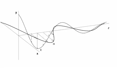
When waves propagate in a charge-free partially conducting medium (σ≠ 0), the wave equations become homogeneous Helmholtz type equations in which a propagation constant (γ) is added (Equation 2.2.9). These materials are called lossy dielectrics due to the loss of

electromagnetic energy into heat. Figure 2.2.1 shows a typical wave penetration in a lossy dielectric. 0 t2 2 2 2 ₌ ∂ ∂ γ −

∇ E E [2.2.9]

where the propagation constant is defined according to the following equation: )

j ( j

2 _{= ωµ σ+ ωε}

Figure 2.2.1. Propagation of electromagnetic waves in a dielectric material

Since γ is a complex quantity it can be written as shown in equation 2.2.10a. Where α is known as the attenuation constant and measures the spatial decay of the wave as it propagates (equation 2.2.10b). And β is a measure of the phase shift per unit length and is called the phase

constant or wave number (equation 2.2.10c). Both α and β are dependent on the frequency of the wave, and the conductivity and permittivity of the material through which the wave propagates.

β + α =

γ j [2.2.10a]

    

  

−    

ωε σ + µε ω =

α 1 1

2

2

        +     ωε σ + µε ω =

β 1 1

2

2

[2.2.10c]

where the propagation velocity and wavelength are dependent on β as follows:

β ω =

u [2.2.11]

β π =

λ 2 [2.2.12]

One of the most interesting observations from the previous analysis is that the electric and magnetic fields E and H are out of phase. Which means that at any time, E leads H by an angle θ/2, known as loss angle. This phase-shift of the fields is a result of the complex intrinsic impedance of the medium, and by analyzing the magnitude of the current density to the

displacement current, the loss angle is defined as follows.

ε ω

σ = θ

tan [2.2.13]

Due to the lossy nature of dielectric materials, the permittivity of such materials can also be written as a complex quantity. The tangent of the loss angle is equivalent to the ratio of the imaginary and the real part of complex permittivity, and is as follows:

" j ' j

1

c =ε− ε

     ε ω σ − ε =

This is called the complex dielectric constant and it is usually reported as a factor of the permittivity of free space. The real part relates to the capacity of the material to store

electromagnetic energy and the imaginary part the losses of electromagnetic energy (Metaxas and Meredith, 1983; Sadiku, 1995; Shadowitz, 1975).

The propagation of electromagnetic waves in a lossless dielectric (σ << ωε) is similar to the propagation of electromagnetic waves in free space. In this case, α = 0 so that there is no attenuation in the field energy and the loss tangent is 0, and H and E are in phase.

In a good conductor (σ << ωε), the loss tangent tends to infinity, and E and H will be out of phase by 45°. The electromagnetic wave loses energy very quickly generating what is called a skin effect. Both E and H will be attenuated by a factor e-αz. Penetration depth is defined as the depth where the wave amplitude becomes 1/e of the original. In the case of good conductors, the penetration depth (δ) is defined as (Sadiku, 1995):

σ µ π = α = δ

f 1 1

[2.2.15]

The penetration depth is an important parameter to analyze and describe the behavior of electromagnetic waves inside a material, but due to the finite dimensions of the material being processed in a microwave system, it becomes necessary to analyze the behavior of the waves when there are changes in the propagation medium.

2.2.1.4 Electromagnetic waves in interfaces

constitutive properties of the two materials (µ, σ, ε) and on the angle of incidence of the waves. The intrinsic impedance (η) of the medium is one of the parameters required to study this phenomena, and it is defined as:

2 / j

j _{= η∠θ}

ωε + σ

ωµ =

η [2.2.16]

For perfect conductors, η = 0 while for perfect dielectrics, η→∞.

The loss tangent is related to the intrinsic impedance (Equation 2.2.16), and it can also be noticed from equation 2.2.16 that for any medium, the electric and magnetic fields are related by the intrinsic impedance such that:

η = E

H [2.2.17]

At the interface of any two materials, the boundary conditions require that both E and H be continuous, so that the component of the fields that are tangential to the interface must follow a continuity equation of the form:

t r

i E E

E + = [2.2.18a]

t r

i H H

H + = [2.2.18b]

From this it can be shown that:

i 2 1 1 2 r E E η + η η − η

= [2.2.19]

and _i

2 1 2 r 2 E H η + η η

Since part of the electromagnetic wave incident at an interface will be transmitted and some reflected, reflection (Γ) and transmission (τ) coefficients are defined. Both coefficients are dependent on the intrinsic impedance of the different mediums, and are dimensionless quantities, but can be complex numbers. The values of Γ range between 0 and 1.

2 1 1 2 η + η η − η =

Γ [2.2.21]

2 1 2 2 1 η + η η = Γ + = τ [2.2.22]

When waves are enclosed within walls made of a conducting material and are allowed to reach steady state, a certain portion of the waves is reflected from the interface and a portion is transmitted. Thus, a standing wave is formed, in which the intensities of the electric and magnetic fields add and form a wave that apparently does not travel. The standing wave is a function of the reflection coefficient of the interface, and of the form of the incident and reflected waves. The ratio of the maximum to the minimum electric or magnetic field is called the

standing wave ratio (s) and is defined as follows:

Γ − Γ + = = = 1 1 s min max min max H H E E [2.2.23]

From this definition, and given that s is easier to measure than E or H, or the reflection coefficient, an alternative method to calculate Γ has been derived as follows:

This is a more useful definition since the standing wave ratio is easier to measure than the reflection coefficient (Sadiku, 1995; Shadowitz, 1975; Rothwell and Cloud, 2001).

The electromagnetic concepts studied in this section, have been developed for

communications and radar but they can be applied to food applications as well. The application and understanding of these concepts in industrial food application is necessary to improve the acceptance and of this technology in the industry.

2.3 Microwave heating of food

The use of microwaves to heat foods has become common in the American household. The microwave oven has become a common appliance in American kitchens, and it is

commercially available in many variations, sizes, and powers. The frequency at which these microwave ovens operate has been regulated by the Federal Communication Commission due to the use of microwaves for communications, and radar. The allocated frequencies for industrial, medical, and household applications are 915 ± 13 MHz, 2450 ± 50 MHz, 5800 ± 75 MHz, and 24125 ± 125 MHz for industrial, scientific and medical applications (47CFR18.301, 2004). A frequency of 2450 MHz is used mostly in household microwave ovens, while 915 MHz is intended for industrial applications.

Conventional heating relies on heat transfer to the product from a hot or to a cold

- Power can be turned on and off instantly - It is very rapid

- It does not rely on contact with hot surfaces or a hot medium

- It is selective, i.e. different materials, or portions of the same food material having different properties will heat at different rates

- It is volumetric, thus theoretically more uniform than conventional heating

With all these considerations, Microwave heating is a promising technology for heating of food materials that are difficult to heat conventionally. However, observations show that microwave heating does not heat food uniformly. This lack of uniformity is due to several factors such as geometry of the microwave oven cavity, thermal and dielectric properties of the food, frequency used, etc. The development of microwave heating of foods has faced several challenges and setbacks over the years, mainly due to the observed lack of uniformity of heating of food materials. Thus, the mechanisms of heating of foods when exposed to a microwave field need to be investigated in more detail (Metaxas and Meredith, 1983; Datta and Anantheswaran, 2001).

2.3.1 Heating mechanisms of foods

accepted that water and ions (polar molecules) are the responsible for the ohmic loss of microwave energy within a food, as stated in equation 2.2.4 (Nelson and others, 1994). This statement maybe related to the mobility of ions, which in the absence of water, is very restricted.

The dielectric properties of the material, introduced in equation 2.2.12 are the properties that relate the ability of the food materials to be heated using microwaves. Food materials comprise a wide variety of dielectric properties, and it can be observed in compilations by Kent (1987), Funebo and Ohlsson (1999), Nelson (1991), and Nelson and others (1994). Due to this wide range of dielectric properties, it becomes very difficult to devise an apparatus or application that would be universal. Thus, many specific applications have been devised in the food

industry.

2.3.2 Applications in the food industry

Applications of microwave heating in the food industry are slowly gaining acceptance. The applications that have initially succeeded in being adopted widely are shown in table 2.3.1.

Table 2.3.1 Current applications of microwave heating in the food industry. (Adapted from Datta and Anantheswaran, 2001)

Product Unit operation

Pasta, onions, herbs Drying

Bacon, meat patties, chicken, fish sticks Cooking

Fruit juices Vacuum drying

Frozen foods Tempering

Surimi Coagulation

2.3.3 Components of a microwave heating system

A microwave heating system, either batch or continuous, is composed of the following elements: Microwave source, directional coupler, waveguide, heating chamber, and control & safety elements. The microwave source can be a magnetron, a klystron type tube, or a solid state microwave generator. The waveguide is a conduit through which the microwaves are conducted to the heating chamber, where the food is placed and heated. The control elements include timers and power controllers, and safety elements are required to avoid the exposure of microwaves to the operators.

2.3.3.1 Magnetrons

back to the development of radar equipment during World War II. A magnetron can be defined as a vacuum diode, made up of circular resonant cavities around a cathode immersed in a perpendicular magnetic field. The perpendicular magnetic field forces the electrons emitted by the cathode into a curved motion, which is very efficient in converting DC energy from the electrons into microwave energy. There are two types of magnetrons, pulsed and continuous wave magnetrons. Pulsed magnetrons are used in radar applications and have a very high peak power output for a very short time. Continuous wave magnetrons are the ones used in most heating application and have a continuous power output at the expense of peak output (Ishii, 1995).

by water cooling in industrial applications. The output of a magnetron is a mean to couple the energy from the magnetron to the waveguide, it consists of a loop in one of the resonant

chambers or a coaxial conductor connected to a vane (Metaxas and Meredith, 1983; Ishii, 1995). The power of a magnetron has to be varied and controlled in order to deliver power precisely and effectively. Several methods are available to control the output of the magnetron, which include:

• Pulsing the output of the magnetron is the method used in most household microwaves, in which the magnetron is turned on and off in intervals to control the average power delivered to the load. The pulse cycles can be in the 2-20 s range. This method is not compatible with continuous heating, as it will not expose the product to the microwaves uniformly but is used in household microwave ovens.

• Changing the Anode Current, it has been proved that the output power of a microwave is directly proportional to the anode current. However, there is a minimum voltage that needs to be applied to the anode, it is called Hartree voltage and is dependent on the magnetic field, anode radius, cathode radius, and the wavelength. Most power supplies are normalized to a certain voltage that will be higher than the Hartree voltage to avoid this pitfall.

The conversion of electric energy into microwaves is very efficient, but some of this energy is spent as heat. The efficiency of a magnetron is thus defined by the amount of heat that must be removed. Current magnetrons operate with efficiencies ranging from 70 to 85% (Ishii, 1995).

The produced microwave energy inside the magnetron has to be conveyed to the product in the heating chamber. A method that delivers power from the microwave source to the heating chamber in a very efficient manner has been found in the use of waveguides.

2.3.3.2 Waveguides

While having electromagnetic waves in open space can be useful for broadcasting media, such as TV or radio, a method for propagating the waves in a more orderly manner is more appropriate for other applications. In order to transmit power or information efficiently, guided structures are used. These structures help to guide the electromagnetic waves from the source to the load in a direct manner; examples of these structures are transmission lines and waveguides (Sadiku, 1995).

While transmission lines can only support transverse electromagnetic waves, waveguides can support many possible field configurations. Moreover, transmission lines can be used from DC to a certain frequency, while waveguides can only be used above a certain frequency acting as a high frequency filter. This characteristic makes them useful for high frequency

electromagnetic waves, such as microwaves and radio frequency (Ishii, 1995; Sadiku, 1995; Cronin, 1995).

Rectangular waveguides are used more often in microwave heating, due to construction and wave transport considerations. In order to analyze what happens in a waveguide the following assumptions are made: the walls are made of perfect conductor (σ ~ ∞), the material in the inside is a perfect lossless dielectric (σ = 0), and no charges are found in the waveguide.

The coordinate system used has z as the direction of propagation of the wave, x and y as the dimensions of the waveguide. The resulting field equations are Helmholtz homogeneous differential equations in Cartesian coordinates, like the ones shown in equation 2.2.9, such that:

0

2 2 _{+γ =}

∇ E E [2.3.1a]

0

2 2 _{+γ =}

∇ H H [2.3.1a]

By using Cartesian coordinates (x, y, z) the system of equations 2.3.1 lead to a system of 6 partial differential equations and 6 unknowns (Ex, Ey , Ez , Hx, Hy, Hz). This system can be

solved by separation of variables. The resulting equation for each field component is in the following form: 0 z y x z 2 2 z 2 2 z 2 2 z 2 = γ + ∂ ∂ + ∂ ∂ + ∂ ∂ E E E E [2.3.2]

Z(z) Y(y) X(x)

E_z = [2.3.3]

After applying a separation constant and remembering that the wave propagates in the z-direction, equation 2.3.1 separates as:

0 γ 0 γ 0 γ 2 2 Y 2 x = + ′′ = + ′′ = + ′′ Z Z Y Y X X [2.3.4]

This results in electric and magnetic fields components in the following form:

z y 4 y 3 x 2 x 1

z (A cosk x A sink x)(A cosk y A sink y)e γ −

+ +

=

E [2.3.5]

z y 4 y 3 x 2 x 1

z =(B cosk x+B sink x)(B cosk y+B sink y)e−γ

H [2.3.6]

The other field components can be deducted by remembering the cross product relationships in Maxwell’s equations and the resulting relationships are

y h j x

h2 2 _∂

∂ ωµ − ∂ ∂ γ −

= z z

x

H E

E [2.3.7a]

x h j y

h2 2 _∂

∂ ωµ − ∂ ∂ γ −

= z z

y

H E

E [2.3.7b]

y h j x

h2 2 _∂

∂ ωµ − ∂ ∂ γ −

= z z

x

E H

H [2.3.7c]

x h j y

h2 2 _∂

∂ ωµ − ∂ ∂ γ −

= z z

y

E H

H [2.3.7d]

where 2

y 2 x 2 2

2 _{k k k}

h =γ + = +

From the equation set 2.3.7 it can be derived that several standing wave and field

called modes. These modes of the electric and magnetic fields have been classified in 4 categories as follows (Sadiku, 1995):

1. Transverse electromagnetic modes (TEM), both E and H fields are transverse to the propagation of the wave [Hz = Ez = 0]. But if this

happens, all other components of the field vanish. Thus, TEM modes are not supported by rectangular waveguides

2. Transverse electric modes (TE). [Ez = 0]. The remaining components of

the electric field are transverse to the propagation of the wave, while the magnetic field is parallel to the propagation.

3. Transverse magnetic modes (TM). [Hz = 0]. The remaining components

of the magnetic field are transverse to the propagation of the wave, while the electric field is parallel to the propagation of the wave

4. Hybrid modes. Ez≠ 0 and Hz≠ 0 Neither the electric or magnetic field are

transverse to the propagation of the wave

The TE and TM modes are the preferred modes of propagation, because it is easier to control the fields into them. The propagation constant and phase velocity depend on the mode, and the definition of the constant h2 _{is very important.}

In the case of TE modes, when the electric field is transverse to the propagation of the waves (Ez = 0), the field equations can be solved taking into account the boundary conditions,

x = 0 Ey = 0

0 x =

∂

∂H_z [2.3.8a]

x = a Ey = 0

0 x =

∂

∂H_z [2.3.8b]

y = 0 Ex = 0

0 y =

∂

∂H_z [2.3.8c]

y = b Ex = 0

0 y =

∂

∂H_z [2.3.8d]

The resulting components of the electromagnetic field are shown in equation set 2.3.9 and to satisfy the boundary conditions cos (kx x) and sin (ky y) have to be zero, thus kx and ky can

be written as periodical functions of π/a, affecting the way both h2 and γ are defined, as shown in the system of equations 2.3.10.

0

E_z = [2.3.9a]

z

o y e

b n sin x a m cos

H  −γ

     π       π = z H [2.3.9b] z o

2 _b y e

n sin x a m cos H b n h

j _ −γ

     π       π       π ωµ = x E [2.3.9c] z o

2 _b y e

n cos x a m sin H a m h

j _ −γ

     π       π       π ωµ − = y E [2.3.9d] z o

2 _b y e

n cos x a m sin H a m h γ −       π       π       π γ = x H [2.3.9e] z o

2 _b y e

,... 2 , 1 , 0 n ,... 2 , 1 , 0

m= =

m and n define the different standing wave patterns in the waveguide, and represent the half cycle variations in the x and y direction respectively. Note that if m = n = 0 all the fields components vanish and no propagation is possible. From equations 2.3.5 and 2.3.6 it can be observed that the definition of γ2 _{depends on how k}

x and ky are defined, for propagation in

waveguides these were defined as periodical functions. The propagation constant is also a

function of h, and remembering that k=ω εµ such that:

b n k and a m

k_x = π _y = π [2.3.10a]

2 2 2 y 2 x 2 b n a m k k h       π +       π = +

= [2.3.10b]

εµ ω +       π +       π = γ 2 2 2 2 b n a m [2.3.10c]

Therefore the value of the propagation constant of the wave defines 3 cases of propagation within a waveguide as follow (Sadiku, 1995; Ishii 1995; Cronin, 1995):

1. γ = 0 In this case there is no propagation, so we have the cutoff frequency, that is defined as:

2 2 c _b n a m 2 1 f       π +       π εµ π

= [2.3.11]

2. γ < 0 when the frequency is less than the cutoff. In this case the wave is evanescent and no propagation can occur

3. γ > 0 when the frequency is greater than the cutoff. In this case the propagation is possible, and the phase constant is defined as

2 2 2 b n a m k       π +       π − =

β [2.3.12]

When the waveguide is filled with a lossless material (µ, ε), the speed of light is defined

as

µε

= 1

u and in the case of air this is equal to c. Therefore, the cutoff frequency can be

written as a function of the speed of propagation:

2 2 c _b n a m 2 u f       +      

= [2.3.13]

The impedance of the waveguide can be defined based on the cutoff frequency of the

waveguide, as well as the intrinsic impedance of the medium

ε µ =

η′ . The effective impedance

of a rectangular waveguide is a function of the frequencies as well, as follows:

2 c TE f f 1       − η′ = η [2.3.14]

Rectangular waveguides, when a > b, operate preferentially in single mode. The modes with the lower cutoff frequency are TE10 and TE20 respectively and the dimensions of the

mode is TE10, in this mode the components of the fields that are not zero are Ey, Hx, and Hz

(Cronin, 1995).

The power that a waveguide can transmit in the z direction is given by a surface

integration of the z-component of the Poynting vector and for the TE10 mode it can be calculated

as follows:

b a 2 H

P a 3

0 x b 0 y 2 2 o z

∫ ∫

= E H [2.3.15]

The material of the walls can cause losses of power in the transmitted microwaves, this occurs when the materials is less than a perfect conductor.

Table 2.3.2 Standardized dimensions for rectangular waveguides for use in microwave heating (Adapted from Ishii, 1995)

Frequency range (GHz)

Cutoff frequency (GHz)

Inside dimensions (*10-3 m)

0.32 – 0.49 0.256 584.2 , 292.1

0.75 – 1.12 0.605 247.65 , 123.83

0.96 – 1.45 0.766 195.58 , 97.79

1.70 – 2.60 1.372 109.22 , 54.61

2.20 – 3.30 1.736 86.36 , 43.18

2.3.3.3 Impedance matching

Impedance is defined as the total passive opposition offered to the flow of electric current. To maximize the transfer of power to the food material, and to keep the standing wave ratio and the reflection at a minimum in microwave heating, the impedance of both the

waveguide and the product has to be matched (Bronwell and Beam, 1947).

Several techniques exist to match impedance, and the literature is abundant. One of such methods, also used in transmission lines, matches a load by using shorted sections of

transmission line, called stubs. By changing the location and length of these stubs, the

impedance of the load is matched. Techniques involving 1, 2, or 4 stubs can match any value of impedance (Ishii, 1995; Reich, 1953).

In the case of waveguides, the matching can be achieved by placing small rods of conductive material at a known distance from the load, these rods act in the same way as the stubs do in transmission lines. The length that these stubs are inserted into the waveguide determines the matching of the load in the cavity (Ishii, 1995).