Regression Function Characterization of Synchronous Machine Magnetization and Its Impact on Machine Stability Analysis

(1)

Scholarship at UWindsor

Electronic Theses and Dissertations Theses, Dissertations, and Major Papers

2012

Regression Function Characterization of Synchronous Machine

Magnetization and Its Impact on Machine Stability Analysis

Saeedeh Hamidifar University of Windsor

Follow this and additional works at: https://scholar.uwindsor.ca/etd

Recommended Citation Recommended Citation

Hamidifar, Saeedeh, "Regression Function Characterization of Synchronous Machine Magnetization and Its Impact on Machine Stability Analysis" (2012). Electronic Theses and Dissertations. 431.

https://scholar.uwindsor.ca/etd/431

(2)

Regression Function Characterization of Synchronous Machine

Magnetization and Its Impact on Machine Stability Analysis

by

Saeedeh Hamidifar

A Dissertation

Submitted to the Faculty of Graduate Studies through the Department of Electrical and Computer Engineering

in Partial Fulfillment of the Requirements for the Degree of Doctor of Philosophy at the

University of Windsor

Windsor, Ontario, Canada

(3)

retained in a retrieval system or transmitted in any form, on any medium by any means

(4)

Regression Function Characterization of Synchronous Machine Magnetization and Its Impact on Machine Stability Analysis

by

Saeedeh Hamidifar

APPROVED BY:

______________________________________________ Tomy Sebastian, External Examiner

Nexteer Automotive

______________________________________________ Arunita Jaekel

Department of Computer Science, University of Windsor

______________________________________________ Jonathan Wu

Department of Electrical and Computer Engineering, University of Windsor

______________________________________________ Govinda Raju

______________________________________________ Narayan C. Kar

______________________________________________ Chair of Defense

(5)

Declaration of Previous Publication

This thesis includes four original papers that have been previously published/

submit-ted for publication in peer reviewed journals/conferences, as follows:

Thesis

Chapter Publication Title Publication Type Publication Status

Chapters 3,6 and its impact on synchronous machine transient stability A novel approach to saturation characteristics modeling

analysis Transaction Published Chapter 3 A trigonometric technique for characterizing magnetic _{saturation in electrical machines} Conference Published

Chapter 4 A novel method to represent the saturation characteristics _{of PMSM using Levenberg-Marquardt algorithm} Conference Published

Chapters 4,5 multifunctional characterization of saturation using A state space synchronous machine model with

levenberg-marquardt optimization algorithm Transaction

Submitted/Under Revision

I certify that I have obtained a written permission from the copyright owner(s) to

in-clude the above published materials in my thesis and have inin-cluded copies of such

copy-right clearances to my appendix. I certify that the above materials describe work

com-pleted during my registration as graduate student at the University of Windsor. I declare

(6)

nor violate any proprietary rights and that any ideas, techniques, quotations, or any other

material from the work of other people included in my thesis, published or otherwise, are

fully acknowledged in accordance with the standard referencing practices. Furthermore,

to the extent that I have included copyrighted material that surpasses the bounds of fair

dealing within the meaning of the Canada Copyright Act, I certify that I have obtained a

(7)

Abstract

Magnetization in the ferromagnetic core significantly affects the performance of

elec-trical machines. In the performance analysis of elecelec-trical machines, an accurate

represen-tation of the magnetization characteristics in the machine model is important. As a part of

this research work, two new mathematical models are proposed to represent the

magneti-zation characteristics of electrical machines based on the measured magnetimagneti-zation

charac-teristics data points. These models can be applied to various kinds and sizes of electrical

machines. The calculated results demonstrate the effectiveness of the proposed models.

The comparison analyses on the proposed models and three different existing models

which have been used in the literature by the researchers validate the fact that these

mod-els can be used as proper alternative for the other modmod-els.

Inasmuch as the omission of magnetization in the machine model has a negative

im-pact on the analysis results, integrating the proposed magnetization models into the

syn-chronous machine mode, can better describe the machine behavior. To aim this goal, as a

(8)

and steady state synchronous machine models. The trigonometric model developed in this

work, has been applied to a conventional synchronous machine model and extensive

sta-bility performance analysis has been carried out. This further reveals the usefulness of the

proposed trigonometric magnetization model and the importance of the inclusion of

mag-netization in stability analysis. The other magmag-netization model developed in this research

is incorporated into a state space synchronous machine model that is used in steady state

(9)

With Love and Gratitude

gÉ `ç _ÉäxÄç `Éà{xÜ tÇw Ytà{xÜ

For Blessing Every Moment of My Life with Their Unconditional Support and Love

and

(10)

Acknowledgements

I would like to express my sincere gratitude to my supervisor, Dr. Narayan Kar; For

his invaluable support, inspiring guidance, and encouragements throughout the course of

this thesis work. I would like to thank him for believing in me and my work and giving

me the opportunity to work as a member of his research team.

I would like to express my gratitude to my committee members, Dr. Arunita Jaekel,

Dr. Govinda Raju, Dr. Jonathan Wu, and Dr. Tomy Sebastian from Nexteer Automotive

for reviewing my thesis and their constructive comments and valuable suggestions to

im-prove this work.

I would also like to thank Ms. Andria Ballo, the Graduate Secretary of Electrical and

Computer Engineering Department at the University of Windsor, for her smiles and love;

and for making my life very easy with her supports during the busiest time of my life.

I am thankful to all my friends and colleagues in the Centre for Hybrid Automotive

Research & Green Energy (CHARGE) for their encouragements and supports. Working

in their friendly company was a wonderful experience.

Deep from my heart, I am grateful to my mother, my father, and my siblings for their

(11)

List of Tables

Table 2.1. Base Quantities Used in the Per-unit System ... 20

Table 2.2. Stator Per-unit Equations ... 20

Table 2.3. Rotor Per-unit Equations ... 21

Table 3.1. Frequencies and Amplitudes of the Calculated Magnetization Characteristics for the Machines under the Investigations ... 60

Table 3.2. Comparison of Chi-Square Error Test for Different Trigonometric Orders and Their

Corresponding DFT Orders for the Machines Used in the Investigations. ... 62

Table 4.1. Ten Sample Magnetization Characteristics Functions and Their Corresponding Coefficients Generatedby the Proposed Method for the Lambton Synchronous Machine ... 79

Table 4.2. Chi-Square Test Results for Different Magnetization Representation Models of the Lambton Synchronous Generator ... 80

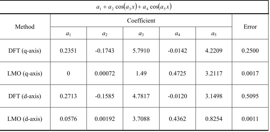
Table 4.3. Coefficients and the Corresponding Errors Calculated for the PMSM Magnetization

Characteristics Using the DFT and LM Optimization Algorithms ... 82

(16)

Table 4.5. Comparison Study on the Magnetization Models Introduced in this Dissertation ... 83

Table 6.1. The First Peak-To-Peak Values of Torque, Load Angle, and Phase Current Calculated by Employing AVR for Model 3. ... 113

Table 6.2. Critical Clearing Time for Different Magnetization Models With and Without AVR. ... 115

Table 6.3. Load Angle and Air-gap Torque Sensitivities with Respect to the Variation in the Machine Parameters. ... 118

Table A.1. The Nanticoke Synchronous Machine Ratings ... 139

Table A.2. The Lambton Synchronous Machine Ratings ... 140

Table A.3. The Lambton Synchronous Machine Parameters ... 140

Table A.4. The DFIG Ratings ... 141

(17)

List of Figures

Fig. 1.1. Typical magnetization characteristics of electrical machines. ... 2

Fig. 2.1. Cross-section view of a two-pole, salient-pole synchronous machine ... 10

Fig. 2.2. Circuit diagram for the rotor and stator of a 2×2 synchronous generator model. ... 11

Fig. 2.3. 22 Synchronous generator model. ... 21

Fig. 2.4. Transient stability concept in power systems. ... 29

Fig. 2.5. A set of flux linkage data points and their corresponding magnetizing currents represented by different degrees of polynomials. ... 30

Fig. 2.6. Mirrored magnetization characteristics calculated by the DFT method. ... 37

Fig. 2.7. Approximated integral calculation in the DFT method ... 37

(18)

Fig. 3.2. The doubly-fed induction generator (DFIG) under the investigations. ... 54

Fig. 3.3. Calculated and measured main flux magnetization characteristics of the DFIG for three orders of trigonometric series and for DFT curve fitting method of order 10. ... 56

Fig. 3.4. Calculated and measured rotor leakage flux magnetization characteristics of the DFIG for three orders of trigonometric series and for DFT curve fitting method of order 10. ... 56

Fig. 3.5. Calculated and measured stator leakage flux magnetization characteristics of the DFIG for three orders of trigonometric series and for DFT curve fitting method of order 10. ... 57

Fig. 3.6. d- and q-axis magnetization characteristics of the Nanticocke synchronous machine presented by the proposed model for two orders of trigonometric series and the 4th_{order of DFT model.}_{... 59}

Fig. 3.7. d- and q-axis magnetization characteristics of the Lambton synchronous machine presented by the proposed model for two orders of trigonometric series and the 4th_{order of DFT model.}_{... 59}

Fig. 4.1. Different configurations to represent magnetization characteristics of a typical electrical

machine. ... 65

Fig. 4.2. Flowchart of the LM optimization algorithm. ... 74

Fig. 4.3. The LM and trigonometric representation of measured data points of the magnetization

characteristics of the Lambton generator. ... 78

Fig. 4.4. The LM and DFT representation of measured data points of the magnetization characteristics of the Lambton generator. ... 78

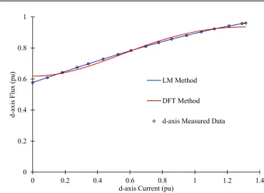
Fig. 4.5. Calculated d- axis magnetization characteristics of the laboratory PMSM employing the LM model and the DFT curve fitting method. ... 81

(19)

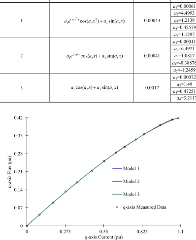
Fig. 4.7. Calculated q-axis magnetization characteristics of the laboratory PMSM employing the LM model

for different functions listed in Table 4.4. ... 83

Fig. 5.1. The dominant eigenvalues for the three magnetization models of the synchronous generator. ... 97

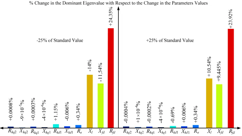
Fig. 5.2. The dominant eigenvalue sensitivity as a function of the variation of the machine parameters calculated by machine model 3. ... 98

Fig. 5.3. The Bode diagram of the speed of the Lambton synchronous machine calculated using magnetization Model 3. ... 100

Fig. 5.4. The Zero-Pole diagram of the speed of the Lambton synchronous machine calculated using magnetization Model 3. ... 100

Fig. 5.5. Frequency response of the synchronous machine speed with respect to the reactive power variations for active power Po=0.9 pu. ... 102

Fig. 6.1. Proposed voltage profile due to a momentary interruption at the machine terminals. ... 107

Fig. 6.2. Air-gap torque calculated by the three synchronous machine models. ... 108

Fig. 6.3. Load angle calculated by the three synchronous machine models. ... 108

Fig 6.4. Load angle response for marginally stable and unstable cases calculated for the three models using proposed trigonometric and DFT method. ... 109

Fig. 6.5. AVR block diagram. ... 110

Fig. 6.6. Machine rotor speed calculated by the three models. ... 111

Fig. 6.7. Synchronous machine air-gap torque calculated by the three models. ... 111

(20)

Fig. 6.9. The synchronous machine phase currents calculated using Model 3. ... 113

Fig. 6.10. Load angle response for marginally stable and unstable cases calculated by the three models. . 114

Fig. 6.11. Peak air-gap torque as a function of fault duration calculated by using Model 3. ... 115

Fig. 6.12. Peak-to-peak load angle sensitivity as functions of different synchronous machine parameters calculated using Model 3. ... 117

Fig. 6.13. Peak-to-peak air-gap torque sensitivity as functions of different synchronous machine parameters calculated using Model 3. ... 117

Fig. 6.14. Harmonic spectrum for the air-gap torque oscillations of the synchronous machine for fault duration of three and half cycles. ... 121

Fig. 6.15. Calculated air-gap torque harmonic spectrum of the synchronous machine by Model 3 for fault duration of four cycles. ... 122

Fig. 6.16. Harmonic spectrum for phase ‘a’ current of the synchronous machine for fault duration of three and half cycles. ... 123

(21)

Nomenclatures

laa, lbb, lcc, : Self-inductance of stator windings

lab, lbc, lca, : Mutual-inductance between stator windings

lafd, lakd, lakq, : Mutual-inductance between stator and rotor windings

Lffd, lkkd, lkkq, : Self-inductance of rotor windings

Ψ : Flux linkage

Im : Magnetizing current

bj, αj, βj : DFT and trigonometric series amplitudes

j,i : DFT and trigonometric series frequencies

k, k’, _{: DFT and trigonometric orders}

aj : LM function coefficients

 : Error criterion

2 _{: Chi-square error} 2 _{: Variance}

λ : Damping factor in LM algorithm

Vt : Steady state terminal voltage

ed, eq : d- and q-axis components of the stator voltage

Xmd, Xmq, : d- and q-axis magnetizing reactances

(22)

 : Saturation coefficient matrix

Ψd, Ψq : d- and q-axis components of the flux linkage

Ψfd,Ψkd,Ψkq : Field and d- and q-axis damper winding flux linkages

Ifd, Ikd, Ikq : Field and d- and q-axis damper winding currents

Rfd, Rkd,Rkq : Field and d- and q-axis damper winding resistances

Xfd, Xkd,Xkq : Field and d- and q-axis damper winding reactances

Ra : Stator resistance

Xl : Stator leakage reactance

B, r : Rated and rotor speeds in electrical radian/second

 : Load angle

KD : Damping torque coefficient

H : Inertia constant

Tm : Mechanical torque input

e,L : Air-gap and load torques

H : Inertia constant

efd : Field voltage referred to the stator

Vt0,Vt1 : Voltage during and after the fault

p-p : Peak-to-peak load angle

p-p : Peak-to-peak air-gap torque

S : Sensitivity with respect to 

N : The number of samples

T : Sampling intervals

W : Window function in STFT

Pm :Mechanical input power

(23)

Chapter 1 Introduction

1.1. Research Background

1.1.1. Magnetization Modeling

Analysis of the non-linear saturation properties of ferromagnetic materials in

electri-cal machines necessitates mathematielectri-cal representation of the flux linkage-current

rela-tionship [1]- [5]. Various mathematical models have been presented by many researchers

that describe the flux linkage and current relationship in electrical machines. The

inclu-sion of magnetization in the electrical machine analysis is important since it affects the

magnetic flux in the direct and quadrature axes. The leakage flux paths are also

(24)

Flux Linkage (pu)

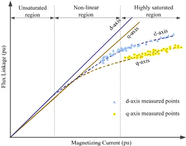
Fig. 1.1. Typical magnetization characteristics of electrical machines.

machines, it is necessary to use a precise and accurate mathematical representation of the

magnetizing saturation. The magnetic flux in the direct and quadrature axes of

synchro-nous machines is influenced by magnetization phenomenon. Thus, it will be useful to

have a synchronous machine model integrated with an accurate magnetization model in

algebraic configuration that makes it valuable in understanding the system behavior [6]-

[24]. Typical magnetization characteristics of an electrical machine is presented in Fig.

1.1. At low magnetizing current values, the flux linkage is proportionately related to the

(25)

current, the flux linkage in the machine reaches its maximum level, which is known as

the highly saturated region. The transition between unsaturated and highly saturated

re-gions takes place in the non-linear region. As illustrated in Fig. 1.1, the flux linkage is not

proportionally related to the magnetizing current in this region [5].

The magnetization model in an electrical machine is a mathematical realization of the

machine magnetization behavior. However, in most of the applications, there is a

collec-tion of experimentally obtained magnetizacollec-tion data points. This informacollec-tion, without

some knowledge of how the current and flux linkage are related, is not useful. Therefore,

employing an algorithm which can create a functional relationship and produce

meaning-ful information will be usemeaning-ful in machine modeling. The various techniques used are

in-tended to address inclusion of magnetization phenomenon into the electrical machine

model [6]- [24].

Researchers have employed numerous methods to incorporate the magnetization

phenomenon into the machine model. A transient saturated model for squirrel cage

induc-tion machines is proposed in [9] based on an assumpinduc-tion that the air-gap flux saturainduc-tion

harmonics are produced by the fundamental component of the air-gap flux. In this model,

the magnetization is included directly by using the fundamental and third harmonic

fac-tors. This model can explicitly be used for induction machines. One particular method

employs variable effective air-gap length [10] to represent magnetization in the machine

model. As a very popular method, the magnetization is expressed by regression of the

(26)

square criterion in [11, 12]. Although this model is very easy to implement, the level of

accuracy is affected by the order of the polynomial. Moreover this method is not

ade-quately accurate when the number of data points is small. To acquire a more accurate

curve in the case of a greater number of data points, a higher degree of the polynomial is

required that results in a more complicated model. On the other hand, increasing the

de-gree of the polynomial will not result in a more accurate regression function and also for

some degrees it might even produce oscillation in the resultant curve. The study

present-ed in [13], [14] includes a set of experimentally measurpresent-ed magnetization characteristics

data points interpolated into rational-fraction functions. This approach to represent

mag-netization is accurate which gives it merit to be considered as a good regression method.

In contrast with the polynomial method, the rational-fraction method generates smoother

and less oscillatory functions. Although the rational method is known as a non-linear

in-terpolation method, it can model a high number of observed magnetization data points

with low degree in both the numerator and denominator. Therefore, in comparison with

the polynomial functions, this method has fewer coefficients. Nevertheless, the main

drawback is that the small number of data points results in some errors in the

magnetiza-tion representamagnetiza-tion.

In [15], a mathematical relationship between magnetism and current is established

using a semi-empirical method. This method can be used for any type of electrical

ma-chine. Nevertheless, since both excessive high and low values of the flux linkage are

(27)

characteris-tic was modeled for induction machines based on the magnetizing current space vector

and generalized flux space vector. A classic hyperbolic function is used in [17] to

inter-polate the -I characteristics of a ferromagnetic core. Although this method can be used

for all kinds of electrical machines, the regression accuracy is not high. Authors in [18],

[19] suggest the magnetic saturation characteristics be divided into three parts in which

the unsaturated and highly saturated regions are expressed as linear functions, while the

saturated part is approximated by an arctangent function. In [5] the same methodology is

employed in spite of the fact that the saturated region is modeled by a hyperbolic

func-tion. Another method proposed by researchers is to express the magnetic flux linkage as a

function of the excitation ampere-turns to represent saturation in the machine model.

However, investigators in these papers made assumptions that may result in substantial

inaccuracies in the determination of the machine performance. Moreover, it is not clear

whether these magnetization models can be applied to all types of electrical machines

[20]. In [21]- [23], the sinusoidal series for modeling data points is presented. In these

papers, the discrete Fourier transform (DFT) approach is used to represent the B-H curve

in transformers based on a discrete set of data points. In the developed model in [24], two

additional sine and cosine terms at half the fundamental frequency are incorporated into

the conventional DFT model to interpolate the data samples to a sinusoidal function.

Alt-hough these models can be used as a general expression of magnetization in any type of

electrical machine, the accuracy of the model is highly affected by the number of the

(28)

By far, the most frequently used methods of regression employed by researchers to

represent magnetization in electrical machine models are polynomial, rational-fraction

and DFT. In the next chapter, the algorithms used to develop the aforementioned methods

are explained in detail. In the subsequent chapters, these models are re-developed and

used to validate the models proposed in this research. It will be shown that these

pro-posed models can be considered as valid alternatives for the existing models to represent

magnetization in electrical machines.

1.1.2. Synchronous Machine Modeling

In performance analysis of electrical machines, it is essential to have a closed-form

mathematical expression that provides a precise description of the system. For a complex

system such as an electrical machine with significant non-linear magnetization properties

of ferromagnetic materials, flux linkage-current relationship must be considered in the

analyses to have more precise and realistic results. Therefore, development of a robust

model based on the available data for magnetization means to increase the accuracy and

reliability of the model [25]. In [18], a synchronous machine model with n number of d-

axis damper circuits and m number of q- axis damper circuits is developed with the

pro-posed magnetization model. In [26], magnetization and hysteresis models are

incorpo-rated into a state space synchronous machine model. A very detailed synchronous

ma-chine model is developed in [27] based on the operating point magnetization specification

(29)

As a part of this research work, based on the proposed magnetization models two

synchronous machine models are developed to be used in steady state and transient

per-formance analysis of synchronous machines.

1.2. Thesis Objectives

The work presented in this thesis conforms to the following objectives:

1. New methods to represent all regions of magnetization characteristics in

syn-chronous machines are developed. These models are capable for application

to all kinds of electrical machines such as synchronous, permanent magnet

synchronous and induction machines. The accuracy of these models is

evalu-ated to ensure the level of reliability.

2. Since having a comprehensive machine model is very crucial to simulating

and analyzing the machine behavior, this research is also focused on

develop-ing transient and steady state synchronous machine models incorporated with

the magnetization models to make the machine model more realistic and

ac-curate. Synchronous machine performance is investigated by conducting

(30)

1.3. Thesis Organization

This thesis consists of six chapters and two appendices

Chapter 2 provides detailed information about the synchronous machine mathemati-cal modeling as well as synchronous machine transient stability performance analysis

theory. Moreover, in this chapter, three models to represent magnetization in electrical

machines that have been used in the literature are introduced and explained in detail.

These models are redeveloped in this research and the results of magnetization

character-istics calculated by these models have been compared with those of the proposed models.

Chapters 3 and 4 present two new magnetization models using trigonometric and Levenberg-Marquardt algorithms, respectively. These chapters consist of the algorithm

development and numerical analyses to validate the accuracy and reliability of the

pro-posed models.

Chapter 5 consists of a comprehensive steady state synchronous machine model in-cluding the magnetization model proposed in Chapter 3.

Chapter 6 studies the magnetization effect on transient performance analysis of syn-chronous machines. The magnetization model developed in chapter 3 is used as the

mag-netization model in the investigations.

Chapter 7 includes the conclusion of this thesis and provides recommendations for future work.

(31)

Chapter 2 Literature Review on the Steady-State and

Transient Analysis of Synchronous

Machines

In this chapter synchronous machine modeling and transient stability analysis are

presented. Additionally, three regression methods used to represent magnetization in

electric machines in the literature are explained in detail.

2.1. Dynamic Synchronous Machine Model

The objective of this section is to introduce the detailed synchronous generator model

which has been used in this research work. In this model for simplicity purposes, it is

as-sumed that magnetization and hysteresis effects are negligible. A cross-section view of a

(32)

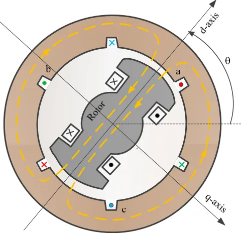
Fig. 2.1. Cross-section view of a two-pole, salient pole synchronous machine

of synchronous machine in this research work is illustrated in Fig. 2.1. As shown in this

diagram, a three phase synchronous machine model consists of three phase stator

wind-ings symmetrically distributed around the air-gap.

The rotor field in synchronous machines is produced by applying a DC current to the

rotor field windings. This results in a sinusoidal distribution of flux in the air-gap of the

synchronous machine. If the rotor is rotated by a prime mover such as a DC motor, a

ro-tating field is produced in the air-gap which is also known as the excitation field. The

in-duced voltages in the armature windings have the same magnitudes but they are 120

elec-trical degrees apart.

To obtain the synchronous generator mathematical model, the rotor reference frame

(33)

respect to the orthogonal axes. By definition, the direct axis is centered magnetically in

the center of the north pole and the quadrature axis lags it by 90 degrees.

The synchronous machine model order is defined by the total number of rotor

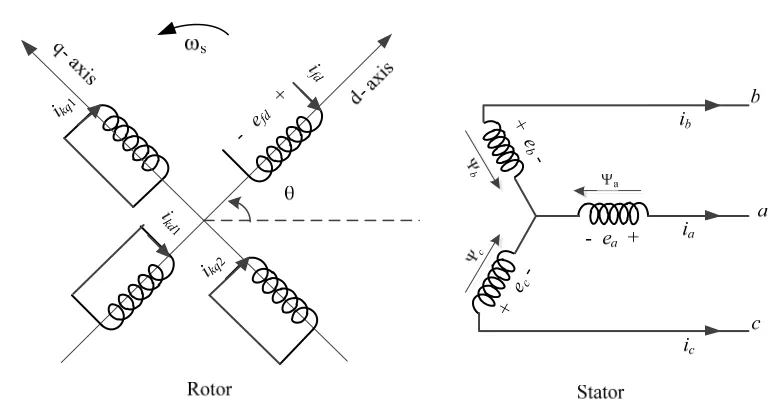
wind-ings on its two orthogonal axes. Fig. 2.2 shows the stator and rotor circuits of a 2×2

syn-chronous machine model used in this research. As shown in this figure, a 2×2

synchro-nous machine model consists of one damper circuit and the field winding along the direct

axis, and two damper circuits along the quadrature axis. Field and damper windings are

also placed along the rotor. As illustrated in this figure, the damper circuits can be

mod-eled by short-circuited windings along the direct and quadrature axes. The angle  is the

rotor position with respect to the stator.

To have a steady torque, the rotating fields of the stator and rotor must have equal

speed which is called synchronous speed. This speed for a p-pole machine is calculated

as

c

b

+

e_b

-+ e c

-fd

fd

kq1

kd₁

kq2

(34)

p p f n s s _  

120 60 (2.1)

where f is the frequency in Hz, s=2f is the angular frequency in rad/s, and ns is the

synchronous speed in rpm.

2.1.1. Stator and Rotor Mathematical Modeling

Assuming that the stator windings are distributed sinusoidally, the mmf wave of each

phase is sinusoidal with 120 electrical degrees apart in space with respect to each

adja-cent phase. Therefore, we have

                  __        __     3 2 cos 3 2 cos cos c c b b a a ki mmf ki mmf ki mmf (2.2)

in which  is the angle along the periphery of the stator and the center of phase a. The

phase current can be defined by

(35)

The total amount of mmf is calculated by



t



kI mmf mmf

mmf

mmf_total _a  _b _c 3 _mcos_s (2.4)

Therefore, the total mmf is a sinusoidal waveform. (2.4) indicates that mmf in

synchro-nous machines rotates at the constant angular velocity of s. Therefore, for a balanced

operating condition in synchronous machine, stator field and rotor must rotate at the same

speed.

Considering Fig. 2.2, the voltage equations for the three phases can be written as

.                      c a c c b a b b a a a a i R dt d e i R dt d e i R dt d e (2.5)

The flux linkages in the three phases are expressed by

. 2 1 1 2 1 1 2 1 1 2 1 1                                                                     kq kq kd fd c b a ckq ckq ckd cfd cc bc ac bkq bkq bkd bfd bc bb ab akq akq akd afd ac ab aa c b a i i i i i i i l l l l l l l l l l l l l l l l l l l l l (2.6)

(36)

. 0 0 0 2 2 2 1 1 1 1 1 1                              kq kq kq kq kq kq kd kd kd fd fd fd fd i R dt d i R dt d i R dt d i R dt d e (2.7)

Since the rotor has a cylindrical structure, the self-inductance of the rotor circuits as

well as their mutual inductances does not depend on the rotor position . Only the mutual

inductances between the rotor and the stator are affected by the rotor position. Therefore,

we have, . 0 0 0 0 0 0 0 0 2 1 1 2 1 2 2 2 2 2 1 1 1 1 1 1 1 1 1 1 1 2 1 1                                                                                     kq kq fkd fd c b a kq kq kq ckq bkq akq kq kq kq ckq bkq akq kd fdkd ckd bkd akd fdkd fd cfd bfd afd kq kq kd fd i i i i i i i l l l l l l l l l l l l l l l l l l l l (2.8)

The stator mutual and self-inductances in (2.8) can be defined by (2.9) and (2.10),

(37)

. 3 2 2 cos 3 2 2 cos 2 cos 2 0 2 0 2 0                   __         __       aa aa aa aa aa aa L L l L L l L L l cc bb aa (2.9) and





                 __                  __     3 2 cos 2 cos 3 2 cos 2 0 2 0 2 0 ab ab ab ab ab ab L L l l L L l l L L l l ac ca cb bc ba ab (2.10) where . 4 2 2 2 0 2 2 2 2 0                                         q d a abl ab ab q d a q d a al P P N L L L P P N L P P N L L aa aa (2.11)

Pd and Pq are the permeance coefficients of the d- and q-axis, respectively and Na is the

(38)

that are not crossing the air-gap. Similarly, the stator-rotor mutual inductances can be

de-fined by (2.12):

. sin sin cos cos 2 1 1 2 1 1                       akq akq akd afd L l L l L l L l akq akq akd afd (2.12)

Equation (2.8) completely describes the mathematical equation of a synchronous

ma-chine. However, it contains the stator currents and the d- and q-axes currents which result

in a very complex calculation.

2.1.2. Park’s Transformation Model

One of the most widely used methods to convert the stator quantity values such as

voltage, current, or flux into their corresponding rotor quantity values is Park’s

transfor-mation [28], This transfortransfor-mation can be defined by the following matrix equation

(39)

in which  can be replaced by voltage, current, or flux. It should be noted that under the

balanced condition we have

0     

_a _b _c (2.14)

Therefore, 0=0. The inverse transformation can be defined as:

                                                                __        __                         0 1 3 2 sin 3 2 cos 1 3 2 sin 3 2 cos 1 sin cos q d c b a (2.15)

2.1.3. Rotor Reference Frame Equations

Using the transformation equation in (2.13) to convert the flux linkages and currents

in (2.6) and (2.8), one can obtain

                                                              0 2 1 1 0 2 1 1

0 0 0 0 0 0 0

0 0 0 0 0 0 0 0 i i i i i i i L L L L L L L kq kq q kd fd d akq akq q akd afd d q d (2.16)

(40)

                    0 0 2 0 0 2 0 0 2 2 3 2 3

0 aa ab

aa ab aa aa ab aa L L L L L L L L L L L q d (2.17) and . 2 3 0 0 0 2 3 0 0 0 0 0 0 2 3 0 0 0 2 3 2 1 1 2 2 1 2 2 1 1 1 1 1 1 1 2 1 1                                                                                 kq kq q kd fd d kq kq kq akq kq kq kq akq kd fd kd akd fd kd fd afd kq kq kd fd i i i i i i L L L L L L L L L L L L (2.18)

Therefore, stator voltage equations in (2.5) can be converted to d-q components as

fol-lows [1]                            0 0 0 R i

(41)

where r is the angular velocity of the rotor. For the steady state operating situation we have rad/s 377 60 2 Hz 60

@f  _r _s   (2.20)

2.1.4. Power and Torque Equations:

The three-phase output power can be calculated in the rotor reference frame as





. 2 3 q q d d

o e i e i

P   (2.21)

Substituting the voltage component from (2.19) in (2.21), (2.22) can be written as







2



.

2 2 3 loss resistance armature 2 0 2 2 power gap -air energy magnetic armature in change of rate 0 0                            _  _ 

 q _r _d _q _q _d _d _q _a

q d d

o i i i i i R

dt d i dt d i dt d i P                            (2.22)

Consequently, the air-gap torque can be expressed by





. 2 3 power gap -air mech d q q d mech r

e i i

T  

   

 (2.23)

2.1.5. Per-unit Calculations

In lights of the fact that using per-unit system results in simplified computational

analyses, all the performance analyses are conducted in per-unit system in this research.

(42)

. value Base

value Actual unit value

Per  (2.24)

In this work, the machine ratings are chosen as the base quantities in the per unit

cal-culations. Tables 2.1- 2.3 summarize the per-unit equations used in this research. It

should be noted that hereafter all the quantities used in this thesis are in per unit unless

the unit is specified.

2.1.6. The Synchronous Machine d- and q-axis Equivalent Circuits

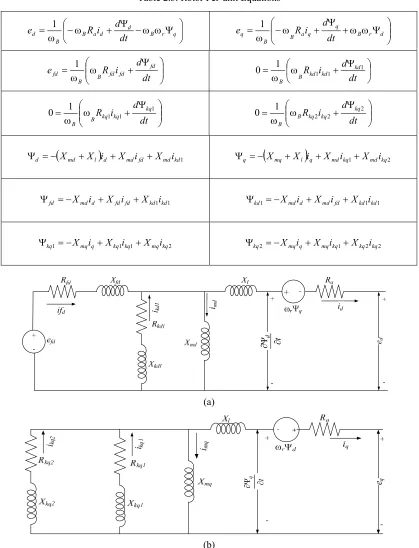
Based on the equations developed in the previous section, Figs. 2.3-a and -b provide

the synchronous machine direct and quadrature axes equivalent circuits, respectively.

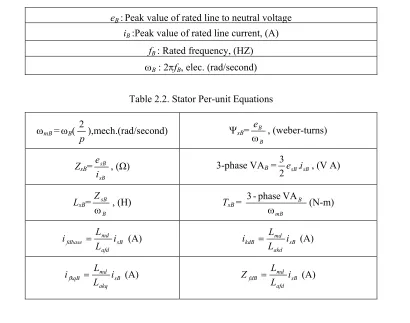
Table 2.1. Base Quantities Used in the Per-unit System

eB: Peak value of rated line to neutral voltage

iB:Peak value of rated line current, (A)

fB: Rated frequency, (HZ)

B : 2fB, elec. (rad/second)

Table 2.2. Stator Per-unit Equations

mB= B(

p

2

),mech.(rad/second) sB=

B B e

 , (weber-turns)

ZsB=

sB sB i e

, (Ω) 3-phase VAB =₂esB.isB

3

, (V A)

LsB=

B sB Z

 , (H) TsB= _mB B 

VA phase -3

(N-m)

(A)

sB afd md fdbase i

L L

i  sB (A)

akd md

kdB i

L L i 

(A)

sB akq md

fkqB i

L L

i  sB (A)

afd md

fdB i

L L

(43)

Table 2.3. Rotor Per-unit Equations        __ __    

 d _B _r _q

d a B B d _dt d i R

e 1 _

             

 q _B _r _d

q a B B q _dt d i R e 1            dt d i R e fd fd fd B B fd 1 _           dt d i R kd kd kd B B 1 1 1 1 0            dt d i R kq kq kq B B 1 1 1 1 0 _           dt d i R kq kq kq B B 2 2 2 1 0



md l



d md fd md kd1

d  X X i X i X i

 q 



XmqXl



iqXmdikq1Xmdikq2

1 1kd kd fd fd d md

fd X i X i X i

 kd1 Xmdid XmdifdXkd1ikd1

2 1

1

1 mqq kq kq mqkq kq X i X i X i

 _kq₂ X_mqi_q X_mqi_kq₁X_kq₂i_kq₂

t d   (a) t q   (b)

(44)

2.2. The State Space Synchronous Machine Model

In this section, a comprehensive saturated model for synchronous machines is

pre-sented. To describe the dynamic behavior of synchronous machines in time domain, the

analysis of this section employs the state space modeling concept. Therefore, based on

the dynamic equations of synchronous machines and their particular state variables, the

state space model can be utilized to determine the future state of the machine provided

that the present state and the excitation signals are known [29]. Firstly, consider a general

non-linear system with multiple states and inputs as



x x xn u u um



f

x_ ₁, ₂,... , ₁, ₂..., (2.25)

where xi is the ith vector of the state variables, uj is the jth system driving variable, and f is

a set of non-linear functions. Suppose the equilibrium points of x0i and u0j are defined

such that f(x01, …, x0n, …, u01, …, u0m)=0. If xiand uj are considered to be a perturbed

state of the above system, (28) can be written as

     

 



  

 



m m m

n n n

u u u u

u u u u u

x x x x

x x x x x

~ ~

~

~ ~

~

0 2

02 2 1 01 1

0 2

02 2 1 01 1



 _{. (2.26)}

Note that at the equilibrium points, the function f is zero. The linearization of the system

about the equilibrium point can be obtained using Taylor series expansion and by

(45)



,... , ,...,



~ ~. 1 ` 1 ` 1 1 0 0 0 0 i n i u ux x i i

n i

u ux x i m n u u f x x f u u x x f x i i i i i i i i                           

 _(2.27)

Therefore, for small perturbation of a non-linear system around the equilibrium point the

linear state space model of the system can be written

       U D X C Y U B X A X (2.28)

in which A,B, C, and D are called the system, input, output, and feed-forward coefficient matrices, respectively. Considering X0 as the initial condition of the system, applying the Laplace transformation to the state space equations in (2.28), we have

 

s ₀

 

s

 

s.

sX X AX BU (2.29)

Therefore,



sIA

  

X s X0 BU

 

s. (2.30)

It yields,

  

s sI A



1X₀



sI A



1BU

 

s.

X       (2.31)

It can be proven that



sIA



1L

 

eAt . (2.32)

(46)

 

   

_{ }

 

_

  

 

  



 

t t

t

d e

e

t t

t t-t-t

U D X C Y

U B X

X A A

0 0

0

(2.33)

2.3. Fault Analysis

In a power system, an abrupt disturbance that causes a deviation from normal

opera-tion condiopera-tions of the power equipment is generally called a fault. Based on the nature of

the fault, they are classified into two groups. The first type of failures is short-circuiting

faults. They may occur as a result of an insulation default in the apparatus due to

degra-dation of electrical components over time or as a consequence of a sudden overvoltage

situation. The other type of faults is categorized under open circuit faults as a result of an

interruption in current flow [30].

In case of short-circuit fault occurrence in the transmission system, the fault must be

cleared in the least amount of time possible to prevent the system from losing the

syn-chronism and becoming unstable [31]. Therefore, part of this research is focused on

per-formance analysis of a synchronous generator when it is subjected to a short-circuit

inter-ruption.

2.3.1. Classification of Short-circuit Faults

Weather conditions are one of the common factors causing short-circuit faults in

(47)

equipment are some of the weather-related conditions that can cause a short-circuit

fail-ure.

Equipment failure due to aging, degradation, or poor installation of the machines,

ca-bles, transformers, etc. can be another cause of short-circuit failure. Short-circuit faults

can also happen as a result of human error. For instance, this fault may happen during the

re-energizing process of the system to be in service after maintenance due to some

inad-vertent mistakes[30], [31].

2.3.2. Effects of Short-circuit Faults on Power System Equipment

The short-circuit effects on the power system equipment can be classified as either

electrical or mechanical effects. Depending on duration of the short-circuit fault, the

cur-rent passing through the conductors of the power system equipment may cause some

thermal effects such as heating dissipations. On the other hand, electromagnetic forces

and mechanical stresses caused by short-circuit interruption are considered to be

mechan-ical effects. Mechanmechan-ical effects of short-circuit failures may result in serious problems.

Therefore, it is essential that the transformers windings are designed to tolerate

electro-magnetic forces. Also, if the cores in a three-phase unarmored cable are not bounded

properly, the electromagnetic force due to the short-circuit fault, can cause the cores to

(48)

2.4. Transient Stability Analysis

In the previous section, short-circuit faults as a common source of failures in power

systems was presented. In this section, transient stability analysis is briefly introduced.

More information for further reading is available in [1], [29].

By definition, transient stability is the ability of a system to sustain synchronism after

it is subjected to sever transient disturbances. Through a part of this research, the

magnet-ization effect on the synchronous generator transient stability in the case of a short-circuit

fault is investigated.

It should be noted that after the fault occurs, the circuit breakers at both ends of the

faulted circuit will be activated to isolate the circuit and clear the fault. The fault clearing

time depends on the speed of time at which the circuit breakers can perform.

Firstly, let us consider fault location F1 to be at the high voltage transmission (HT)

bus as indicated in Fig. 2.4-a. For simplicity it is assumed that the stator and transformer

resistors are small and can be neglected. Therefore, in this situation, no active power is

transmitted to the infinite bus during the fault and the short-circuit current flows through

the pure reactance.

If the fault occurs at location F2 as shown in Fig. 2.4-b, some active power will be

transmitted to the infinite bus during the fault. Figs 2.4-d and 2.4-e demonstrate the active

power P graph with respect to the load angle  for stable and unstable situations,

(49)

Suppose that the system is subjected to the fault at t=t0 and the fault is cleared at t=t1.

First, let us examine the stable situation shown in Fig. 2.4-d. As can be seen in this figure,

before the fault the system operates at the pre-fault state of operation. At t=t0, one of the

circuits is subjected to the fault. Therefore, the operating point suddenly drops from point

a to b. As a result of inertia, load angle cannot suddenly change. Since Pe<Pm, the rotor

starts accelerating until point c, at which the fault is cleared by activation of the circuit

breakers and isolating the faulted circuit from the network. Therefore, the operating point

abruptly changes to point d. At this time, since Pm<Pe, the rotor starts decelerating.

How-ever, the load angle continues increasing because during the fault the rotor speed is

in-creased to more than synchronous speed (0, 0). Therefore, the load angle increases until

the kinetic energy gained by the machine during the acceleration (area A1) is expended.

When the operating point reaches to d (t=t2)at which we have A1=A2 the rotor speed is the

synchronous speed and load angle is maximum. Since Pm<Pe remains true the rotor speed

and the load angle decrease. If there is no source of damping in the network, the

operat-ing point oscillates between points e and d.

With the longer fault duration illustrated in Fig. 2.4-e, the area A1 representing to the

energy gained during the fault is greater than area A2. Therefore, after the fault is cleared

at point e, the kinetic energy is not completely expended in the system. As a result, the

speed and the load angle both increase. The speed never reaches the synchronous speed,

(50)

Based on the above discussion, one can conclude that the transient stability in

syn-chronous generators in short-circuit interruptions is affected by the following factors:

- Load of the generator

- Location of the fault

- Fault clearing time

- Post-fault transmission circuit resistance

- Generator reactance: The greater this reactance is, the greater the peak power; this

results in having less initial load angle.

- Generator inertia: For the generators with greater amount of inertia, the kinetic

energy gained during the fault is smaller

(51)

(a)

G

F2

HT _E_B

F2

E

EB

(b) (c)

(d) (e)

(52)

2.5. The Previous Models Used to Represent

Magneti-zation

In this section, three methods to represent magnetization in electrical machines used

by the researchers are explained. These models are developed in this research work to be

used in comparison investigations to validate the proposed models.

2.5.1. Polynomial Regression Algorithm

Polynomial regression is one of the most commonly used methods in representation

of magnetization characteristics in electrical machines. Fig. 2.5 illustrates a representation

 Im c0c1Im



  3

3 2 2 1

0 m m m

m c cI cI cI

I    



  n

m n m m

m c cI cI cI

I     

 2 _

2 1 0

1,Im1 ,2,Im2 ,,n,Imn

  2

2 1

0 m m

m c cI cI

I   



Fl

ux lin

kage

(pu)

Magnetizing current (A)

(53)

of a set of flux linkage data points and their corresponding magnetizing currents by

dif-ferent degrees of polynomials. In general, n number of data points can be interpolated by

a set of polynomials from a straight line (k=2) to a polynomial of degree k=n-1.

Suppose that for the available set of magnetization data points the function is

ex-pressed in the form of a polynomial of degree k as

 

 ₀  ₁  ₂ 2    ₀   .





k 1 i

i m i k

m k m

m

m c c I c I c I c c I

I _ (2.34)

To assure that the curve is the best-fit curve of the data points, the least square method is

employed. In this technique, the error function is defined as sum of the squared

devia-tions from the data points.

 





.

1

2    





n

j mj j

I (2.35)

Substituting the calculated flux linkage from (2.34), (2.36) can be written as

.

1

2 0

_    _ 



 

n

j j

k 1 i

i mj iI

c

c (2.36)

According to the least square error method [32], [33], the regression algorithm will be

successful if the error is minimized by

. 0

2 1 0

 

    

   

 

k

c c

c

c  (2.37)

(54)

. 0 2 0 2 0 2 0 2 1 0 2 1 0 2 1 0 1 1 0 0                    _   _       _   _       _   _      _   _             k m n j j k 1 i i mj i k m n j j k 1 i i mj i m n j j k 1 i i mj i n j j k 1 i i mj i I I c c c I I c c c I I c c c I c c c  (2.38) Consequently,













. 1 1 1 2 2 1 1 1 1 0 1 1 2 2 1 4 2 1 3 1 1 2 0 1 1 1 1 3 2 1 2 1 1 0 1 1 1 2 2 1 1 0                                                                                     n j n j k m j k k m k n j k m n j k m n j k m n j n

j j m k m k n j m n j m n j m n j n

j j m k m k n j m n j m n j m n j n j j k m k n j m n j m I I c I c I c I c I I c I c I c I c I I c I c I c I c I c I c I c nc     (2.39)

Regression Function Characterization of Synchronous Machine Magnetization and Its Impact on Machine Stability Analysis

Scholarship at UWindsor

Scholarship at UWindsor

Regression Function Characterization of Synchronous Machine

Regression Function Characterization of Synchronous Machine

Magnetization and Its Impact on Machine Stability Analysis

Magnetization and Its Impact on Machine Stability Analysis

Regression Function Characterization of Synchronous Machine

Magnetization and Its Impact on Machine Stability Analysis

Declaration of Previous Publication

Abstract

gÉ `ç _ÉäxÄç `Éà{xÜ tÇw Ytà{xÜ

Acknowledgements

Table of Contents

List of Tables

List of Figures

Nomenclatures

Chapter 1

Introduction

1.1.

Research Background

1.1.1.

Magnetization Modeling

1.1.2.

Synchronous Machine Modeling

1.2.

Thesis Objectives

1.3.

Thesis Organization

Chapter 2

Literature Review on the Steady-State and

Transient Analysis of Synchronous

Machines

2.1.

Dynamic Synchronous Machine Model

2.1.1.

Stator and Rotor Mathematical Modeling









2.1.2.

Park’s Transformation Model

2.1.3.

Rotor Reference Frame Equations

2.1.4.

Power and Torque Equations:

















2.1.5.

Per-unit Calculations

2.1.6.

The Synchronous Machine d- and q-axis Equivalent Circuits









2.2.

The State Space Synchronous Machine Model









 

 

 



  

 

  







 

_{ }