Identification and selection of best fitting candidate distribution for rainfall frequency analysis in Cameron Highlands

1-.-,

,

I

I

i

I

r

i

J. Kej. Awam Ji!. 8 Bi!. 2 1995

IDENTIFICA TION AND SELECTION

OF BEST.FlTTING CANDIDATE DISTRIBUTION

FOR RAINFALL FREQUENCY ANALYSIS

IN CAMERON HIGHLANDS

by

Amir Hashim b. Mohd. Kassim -I

Choi Lim Fatt

-2 Dept. of Hydraulics and Hydrology

Faculty of Civil Engineering

ABSTRACT

In frequency analysis based on analytical method, there are quite a number of probability distributions to be used for quantile estimation. The selection of inappropriate one will lead to either overestimation or underestimation of the quantiles. Thus the identification and selection of the best fitting probability distribution should be given emphasis. The L-moment method offers advantages over the conventional method of moment and thus is more reliable in the distribution identification. The focus of this study is on the identification and selection of best fitting probability distribution, based on L-moment ratio parameters and L-moment ratio diagram. The results show that the GEV (Generalized Extreme Value) distribution fits quite well to data series at most of the homogeneous regions and rainfall intervals.

*1 Head of Hydraulics and Hydrology Department, Faculty of Civil Engineering, Universiti Teknologi Malaysia.

INTRODUCTION

Practitioners usually need to estimate the recurrence of rainfall extreme event at particular magnitudes in certain periods of time. through frequency analysis. This is important as design variable for structures such as reservoirs. spillways. irrigation networks and drainage systems. The estimation involves interpolation and extrapolation of the rainfall records available. In the current practice, the graphical methods based on probability papers are very common among practitioners since several decades ago due to their simplicity. However, the reliability of these methods is in question because the solution has been oversimplified. This could lead to overestimation (which is a waste of money due to overdesign) or underestimation (which could be a threat to human lives as strue;:tures may damage due to underdesign) of the quantiles estimated.

Thus, in order to minimize the extent of these problems, the analytical methods should be used instead of graphical methods. For analytical frequency analysis, the best fitting probability distribution needs to be identified or selected. This part of study will look into this crucial aspect in frequency analysis, which will critically affect the results of quantile estimation later.

OBJECTIVES

This part of study is carried out with the objective of:

a) identifying and selecting the best fitting probability distribution for rainfall frequency analysis in Cameron Highlands.

SCOPE OF WORK

In this part of study, the annual maximum data series (based on water year) of I-day, 2-day, 3-day, 5-day and 7-day intervals from 14 rainfall stations (with 531 station.years of data) in Hulu Telom Catchment and Bertam Catchment, are used. APPENDIX A gives the details of the rainfall stations while APPENDIX C shows the locations. The homogeneous regions with the respective rainfall stations are stated in APPENDIX B, which has been determined in another part of study.

In this part of srudy, the differences of regional L-skewness and L-kurtosis between samples of rainfall data series and the five candidate probability distributions are computed. This will provide a measure about the degree of fitness of those candidate distributions to the sample of data. The distribution with the lowest difference will be selected as the best-fitting one. Meanwhile, the L-moments ratio diagrams are constructed and the regional sample L-skewness and L-kurtosis are plotted into the diagrams for identifying the best fitting distribution. Nevertheless it should be emphasized here that this is only a complementary measure as visual inspection is morc subjective.

Data Screening

Regionalization

Quantile Estimation

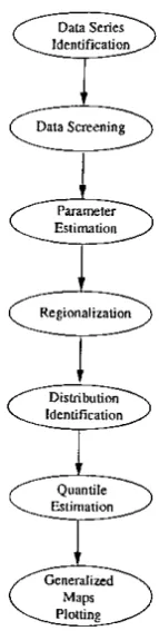
Fig. 1 : Overall Frequency Analysis Procedure in This Study

SOURCES OF DATA

LITERATURE REVIEW

Some studies have been done over the last few years on the application of L-moment method in hydrology, especially in frequency analysis. Vogel and Fennessey (1993) have compared the conventional product moment ratio and L-moment ratio diagram and concluded that product moment estimates of coefficient of variation and of skewness should be replaced by L-moment estimators for most goodness-of-fit applications in hydrology. Pilon et al (1991) concluded from their study and analysis of annual maximum precipitation in Ontario, Canada, for durations ranging from 5 minutes to 24 hours, that the variability in the L-skewness and L-coefficient of variation was primarily due to sampling variability. Pilon and Adamowski (1992) also came to similar conclusion for the study in the province of Nova Scotia, Canada, that by using the L-statistics and simulation, the variability of L-skewness is due in large part to sampling errOL From the studies, it is found that the L-moment method offers some advantages over the product moment method. For instance, it is less sensitive to the effects of sampling variability and outliers, especially in small samples.

Loke (1994)clustered the Klang River Basin (with 20 rainfall stations and 624

station-year of data) into homogeneous regions and computed the L-moment ratio estimators for every region at rainfall with durations of I-day, 2-day, 3-day, 5-day and 7-day. He suggested that the GEV distribution can best fit the regions of different rainfall durations through the usc of L-moment ratio diagram. However, the approach was too subjective because only the visual inspection on the diagrams was done. Instead, the goodness-of-f1t should be judged based on some numerical values that can be computed.

METHODOLOGY

The identification of best fitting distribution is done by comparing the regional L-kurtosis (14), between the sample of rainfall data and the candidate distributions, with L-skewness (t) based on the sample L-skewness. The difference between them is computed and the distribution contributes the least difference in regional L-kurtosis will be selected. Another complementary approach is by plotting the regional sample moment ratio parameters into L-moment ratio diagrams. The identification is done by selecting the candidate distribution with the curve nearest to the sample point.

Under this method, the best fitting frequency distribution is selected from among the following candidate frequency distributions:

a) Generalized Extreme Value (GEV) distribution b) Log-Nonnal (LN) distribution

c) Pearson Type 3 (P3) or Gamma (GAM) distribution d) Generalized Logistic (GLO) distribution

Hosking and Wallis (1993) defined group average L-rnoment. ratios, with N sites weighted proportionally to their record lengths and t/l) as sample L-moment ratios, as

wherer

=

3.4, ..

r

r

N (i)

2:

n.r

I r

i==1

N

2:

n.

I

i=1

(I)

For each of the candidate distributions, the L-kurtosis given

by

Hosking (1990) and Maidment (1993) are as in the equations below.

I

2

where

k ~

7.859d(

1

L

3+r3

CEV

'4

(1_6'2-k

+10'3-k

_5'4-k)

(i_2-k)

:::~ }2955{(3+

2

'3l

log 2]2

log 3

(2)

LN 2 4 6 8

'4

~0.12282+0.77518'3 +0.12279'3 -0.13638'3

+0.11368'3

(3)

P3

2

4

6

8

'4

=0.1224+0.30115'3 +0.95812'3 -0.57488'3

+0.19383'3

(4)

CW

'4

'4 CPA

1- 3'3

where k

=---1+r3

(l-k)(2-k)

(3+k)(4+k)

(5)

(6)

RESULTS AND DISCUSSION

From the previous CFA analysis, the values of sample L-skewness (t3) and L-kurtosis (t4) for all rainfall intervals at each station are obtained. The weighted

APPENDIX D shows the sample calculation for

I-day

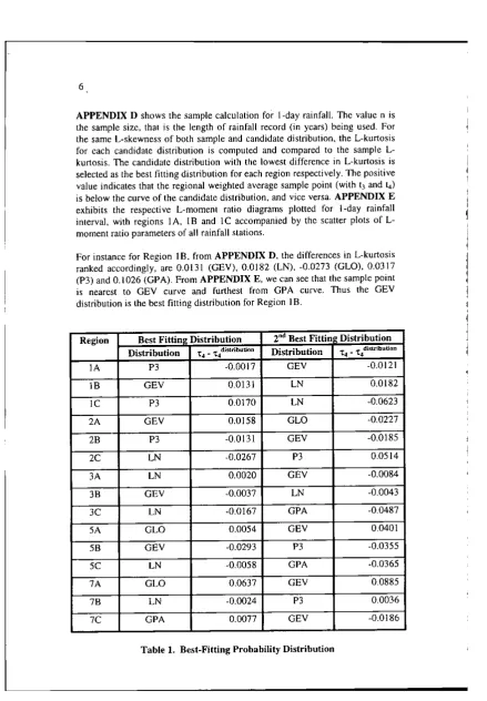
rainfall. The value n is the sample size, that is the length of rainfall record (in years) being used. For the same L.skewness of both sample and candidate distribution, the L-kurtosis for each candidate distribution is computed and compared to the sample L-kurtosis. The candidate distribution with the lowest difference in L-kurtosis is selected as the best fitting distribution for each region respectively. The positive value indicates that the regional weighted average sample point (with 13and 4) is below the curve of the candidate distribution. and vice versa. APPENDIX E exhibits the respective L-moment ratio diagrams plotted for I-day rainfall interval, with regions IA, IBand Ie accompanied by the scatter plots of L-moment ratio parameters of all rainfall stations.

For instance for Region IB. from APPENDIX D, the differences inL~kurtosis ranked accordingly, are 0.0131 (GEV), 0.0182 (LN). -0.0273 (GLO). 0.0317 (P3) and 0.1026 (GPA). From APPENDIX E, we can see that the sample point

is nearest to GEV curve and furthest from GPA curve. Thus the GEV distribution is the best fitting distribution for Region IB.

Region Best Fittine Distribution 2nd_{Best FiUin Distribution}

Distribution t4 - 't4 distribution _Distribution t4 _ t/iSlribution

IA P3 -0.0017 GEV -0.0121

lB GEV 0.0131 LN 0.0182

IC P3 0.0170 LN -0.0623

2A GEV 0.0158 GLO -0.0227

2B P3 -0.0131 GEV -0.0185

2C LN -0.0267 P3 0.0514

3A LN 0.0020 GEV -0.0084

3B GEV -0.0037 LN -0.0043

3C LN -0.0167 GPA -0.0487

5A GLO 0.0054 GEV 0.0401

5B GEV -0.0293 P3 -0.0355

5C LN -0.0058 GPA -0.0365

7A GLO 0.0637 GEV 0.0885

78 LN -0.0024 P3 0.0036

7C GPA 0.0077 GEV -0.0186

As a whole, from Table 1. it is shown that LN distribution is the best fitting distribution for 5 regions while GEV, P3, GLO and GPA are best for 4,3, 2 and 1 regions respectively. The LN distribution should be ranked as the overall best fitting distribution. However, when the differences in L-kurtosis are evaluated carefully, 3 of the 5 regions with the LN distribution as the best are regions C which have only J rainfall station. Thus it is misleading to select the LN distribution as the overall best. Although the GEV distribution dominates only 4 regions, but the regions have more stations. Besides, from Table 1

it

is found that the GEV distribution is the second best fitting for 6 regions. compared to the LN distribution with only 3 regions. Furthermore, for some regions. the difference of GEV distribution is very close to the best fitting distribution. For example, for Region 2B and 3A. the best fitting distributions are P3 (-0.0131) and LN (0.0020) but the second best distribution is GEV (with 0.0185 and -0.0084) respectively. The GEV distribution is selected for regions of most rainfall intervals.

Thus it is more reasonable to say that the overall best fining probability distribution for rainfall frequency analysis in Cameron Highlands is the GEV distribution. In another study, Loke (1994) clustered the rainfall frequencies in Klang River Basin based on 20 rainfall stations (with 624 station-year data) and cop-eluded that the GEV distribution could fit quite well to all the regions of 1-day, 2~1-day, 3-1-day, 5-day and 7-day rainfall. Thus, from the results of both the studies, the GEV distribution has the potential of being adopted as the standard probability distribution for rainfall frequency analysis in Malaysia. Other countries such as United Kingdom. United States of America, Canada and China has adopted Generalized Extreme Value, Log Pearson Type III. 2-Parameter Log-Normal and Pearson Type III distributions respectively. However, the adoption of certain probability distribution for frequency analysis in Malaysia can only be further verified after more studies covering the whole Malaysia being conducted.

CONCLUSION

From the analysis, the best-fitting probability distribution for each region has been identified. Among them the GEV distribution is selected as the overall best fitting probability distribution for rainfall frequency analysis in Cameron Highlands. The quantile estimation will be based on the GEV distribution for all the regions.

ACKNOWLEDGEMENT

REFERENCES

Greenwood, lA. Landwehr, 1.M., Matalas, N.C. and Wallis, J.R. (1979). "Probability Weighted Moments Definition and Relation to Parameters of Several Distributions Expressablc in Inverse Form", Water Resources Research, 15(5): 1049-1054.

Haan,

c.T.

(1977). Statistical Methods in Hvdrolog)', Iowa State University Press, Ames, IA.

Hosking, J.R.M. (1986). "The Theory of Probability Weighted Moments", Res. Rep. ReJ22JO, IBM Research, Yorktown Heights, N.Y. (As cited byHosking and Wallis, 1993)

Hosking, lR.M. (1989). "Some Theoretical Results Concerning L-Moments",

Res. Rep. RC14492, IBM Research, Yorktown Heights, N.Y.

Hosking. J.R.M. (1990). "L.Moments : Analysis and Estimation of Distributions Using Linear Combinations of Order Statistics", 1.R. Statist. Soc.,

52(1): 105-124.

Hosking, J.R.M. and Wallis, J.R. (1993). "Some Statistics Useful in Regional Frequency Analysis", Water Resour. Res., 29(2): 271-281.

Hosking, J.R.M., Wallis, lR. and Wood, E.F. (1985). "Estimation of the Generalized Extreme-Value Distribution by the Method of Probability~ Weighted Moments", Technometrics, 27(3) : 251-261.

Lake, K.W. (1994). Clustering Rainfall Frequencies for Klang River Basin,

Master Thesis, Universiti Teknologi Malaysia.

Maidment, D.R. (Ed.) (1993). Handbook of Hvdrology, McGraw-Hill Inc.,

New York.

Pilon, P.l. and Adomowski, K. (1992). "The Value of Regional Information to Flood Frequency Analysis Using the Method of L-Moments", Can.J.Civ. Eng.,

19: 137-147.

Pilon, PJ.,Adomowski, K. and AIila, Y. (1991). "Regional Analysis of Annual Maxima Precipitation Using L-Moments",Atm. Res., 27: 81-92.

Viessman, W., Lewis, G.L. and Knapp, lW. (1989). Introduction to Hvdrologv, 3rd. Edition, Harper &Row, Singapore.

Vogel, R.M. and Fennessey, M. (1993). "L Moment Diagrams Should Replace Product Moment Diagrams", Water Resour. Res., 29(6) : 1745-1752.

0> ~--::

-;-=

>

~

-2

~2

o

;;.

~>

~

"

'%

"

AI~I'ENIHX E

L_MOMENT RATIO DIAGRAMS

L-MOMENT RATIO DIAGRAM (i-DAY

0.80

0.60

.~ 0.40

~

~ 0.20

0.00

_

.

- - -d:- - - -..-

.-.-.:.D,.; .

...-:~-...~- (i'-" E

N

.•..

U

•

G (Gumbel]

0 E (Exponential)

"

N (Nonnal)

•

U (Uniform)

0 L (Logistic)

--GEV

-.P3@GAM

---LN

GPA

- - - GLO

X Region IA

•• Region lB

• RegionIe

-0.20

-0.20 0.00 0.20 0.40 0.60 o.so

L-SkewIIl.'1is

L~MOMENT RATIO DIAGRAM (l-DA Y)

0.80

0.60

.~OA(}

~

..J_{O_20}

0.00

.~ .

• G (Gumbel) a E (Exponential)

tJ. N (Normal) II U (Uniform)

{} L (Logistic)

--GEV

- _. P3@GAM

- - LN

.CPA

- - - GLO

• Cameron Highl~nds

-0.10

~0.20 0.00 0.:0 0.40

L_Skewne:l5

L-MOMENT RA.TIO DIAGn:;\j\.1 (2-DAY

0.60 0.30

x Region 2A

..

Region 213

•

Region 2C • G (Gumbel)

o E(Exponcnli.iI)

l!. N (Nonn:!!)

t:l U (Unif01m)

o L(Logistic) --GEV _. - - P3@GAM

- .. -IN

.... - -OPA

- - - GLa

.0' E ____ -<>L --:

: '--- •• G

N

0.00 .. _ .•....

U

0..10

.~

~

~ 0.20

-0.20

-0.:::0 0.00 0.20 0.40 0.60 0.80

L-MOMENT RAnD DIAGRAM (2-DA Y)

0.30

0.60

0.00

•

•

_ l

.,--- .,--- .,---<>.,--- .,--- ~ •...

-''-'-

,;c...

Ne ~' •

• 1m" • - •••

u

-' /,"

..

/"

-

...•.

:0-"'

E

• G (Gumbel)

D E (E."ponemi'll) 6. N (Narrnnl)

!lII U (Uniform)

<> l. (Logistic) --GEV

-'P3@GAM - LN

GrA

--- GLD

• Cameron Highlands

-0.20

-0.20 0.00 0.20 0..10 0.60

o,so

(J.110

0.60

DAD

.~

~

~

0.20

0.00

L.MOMENT RATIO DtAGRAM (3-DA Y

,

.,

~

_~

.'

----

."

....

"."

____ -<;>L_ _ __ _.;.:-- •

..-,:...- -'-G--' E

N

.-.•....

u

• G (Gumbel) o E(Exponenlial)

I:. N (Nanna!) • U (Uniform)

() L (Logistic)

--GEV

. - - P3@GAM

--- LN

. _ .. -.CPA

- - - GLC

x RcgiOll 3A

..

Region 38

•

Region 3C

-0.20

-0.20 0.00 0.20 0.40 0.60 OJto

L-S"cwn~ss

L-MOMENT RATIO DIAGRAM (3-DA Y)

0.80

0.60

_~ 0.40

•

~

~0.20

0.00

~-~::-:!:.~~-'~~~

..•....

. m- ..

U

• G (Gwnbcl)

o E(Exponenliill)

I:. N{Nomlal)

II U(tJnironn)

0' L (Logislic)

--GEV --.P3@GAM

.. - LN . ... CPA

- - - GLa

• Cameron Highlands

-ll~O

-0.20 0.00 0.20 O..lO

L-Sl,cwncss

0.60 G.SO

..;{

,'/

.,

./"" 0.80

0.60

~

0.40

~

~

0.10

0.00

/. "'/. "",'

..-;:' '"

y.-- ..

-.:-.-- -<;,L - - _' - ..cr'

:'--- G '-. E N ::

...•...

U

o E(E.~poncllli3J)

0. N (Nonnal)

II U (Unironn)

<> L (Lol,\istie)

--GEV ~-'P3@GAM .. - LN

•... GPA

- - - GLO

x Region 5A

..

Region 58

•

Region 5C

.0.20

.0.20 0.00 0.20 0..10 0.60 0.80

L-SluWDCSS

L-MOMENT RATIO DIAGRAM (5-DA Y)

o,so

0.60

.~O.'lO

~

...l0.20

0.00

• G(Gumbel)

a E (Exponential)

II N (Nonnal)

III U (Uniform)

<> L (I.ogi~lie) --GEV

. _. P3@GAi'v1 .. - LN ... GPA

- - - GLO

• Cameron Highlands

I

j

-0.20

.0.20 0.00 0.<10

L-Skewness

0.80

0.60

.g

0.'10

"

~

...l 0.20

L-MOMENT RATIO DIAGRAM (7-0,\ Y

x

_.

./.

l

:-- - - -0- - -: - . '':_'~DEC

: '--- _.(f

N

• G (Gumbel)

a E (Exponcmial)

A N (Nonnal)

• U (Uniform)

o L(Lo!!,iSLi~)

--GEV

. _. P3@GAM

.. - LN

... CPA

- - - GlO

x Region 7A

..

Region 7n

•

Region 7C

0.00 _1:1' - •••••

u

-0.:!0

.0.20 O.()(J 0.20 0.40 0.60 o.so

L_Skewness

L-MOMENT RATIO DIAGRAM (7-0A Y)

0.30

• Cam~ron Highlands

• G (Gumbel)

o E(E.'l:pon~l1lial)

tJ. N (Nonnal) • U (Unitbml)

o L(logislic)

--GEV '-'P3@GAM _._- LN

... GPA

- - - GlO

•

••

•

.

/

~:.__

-~--e~:i-:'--

~:--N ••

• Ill ••••••••

U

O.()(J

0.60

...,0040

~

:2

_,

-o.:!o

0.00 0.20 0.'10

L-Skewness