Big Data Mining to Construct Truck Tours

(1)

University of Windsor University of Windsor

Scholarship at UWindsor

Electronic Theses and Dissertations Theses, Dissertations, and Major Papers

12-12-2018

Big Data Mining to Construct Truck Tours

Vidhi Kantibhai Patel

University of Windsor

Follow this and additional works at: https://scholar.uwindsor.ca/etd

Recommended Citation Recommended Citation

Patel, Vidhi Kantibhai, "Big Data Mining to Construct Truck Tours" (2018). Electronic Theses and Dissertations. 7620.

https://scholar.uwindsor.ca/etd/7620

This online database contains the full-text of PhD dissertations and Masters’ theses of University of Windsor students from 1954 forward. These documents are made available for personal study and research purposes only, in accordance with the Canadian Copyright Act and the Creative Commons license—CC BY-NC-ND (Attribution, Non-Commercial, No Derivative Works). Under this license, works must always be attributed to the copyright holder (original author), cannot be used for any commercial purposes, and may not be altered. Any other use would require the permission of the copyright holder. Students may inquire about withdrawing their dissertation and/or thesis from this database. For additional inquiries, please contact the repository administrator via email

(2)

Big Data Mining to Construct Truck Tours

By

Vidhi Patel

A Thesis

Submitted to the Faculty of Graduate Studies

through the School of Computer Science

in Partial Fulfillment of the Requirements for the

Degree of Master of Science

at the University of Windsor

Windsor, Ontario, Canada

2018

c

(3)

Big Data Mining to construct Truck Tours

By

Vidhi Patel

APPROVED BY:

H. Maoh

Department of Civil and Environmental Engineering

P. Zadeh

School of Computer Science

M. Kargar, Co-Advisor

J. Chen, Advisor

(4)

DECLARATION OF ORIGINALITY

I hereby certify that I am the sole author of this thesis and the intellectual content of this

thesis is the product of my own work and that no part of this thesis has been published or

submitted for publication.

I certify that, to the best of my knowledge, my thesis does not infringe upon anyones

copyright nor violate any proprietary rights and any ideas or techniques and all the

as-sistance received in preparing this thesis and sources have been fully acknowledged in

accordance with the standard referencing practices. Furthermore, to the extent that I have

included copyrighted material that surpasses the bounds of fair dealing within the meaning

of the Canada Copyright Act, I certify that I have obtained a written permission from the

copyright owner(s) to include such material(s) in my thesis and have included copies of

such copyright clearances to my appendix.

I declare that this is a true copy of my thesis, including any final revisions, as approved

by my thesis committee and the Graduate Studies office, and that this thesis has not been

(5)

ABSTRACT

Cross-Border shipping of goods among different distributors is an essential part of

trans-portation across Canada and U.S. These two countries are heavily dependent on border

crossing locations to facilitate international trade between each other. This research

con-siders the identification of the international tours accomplishing the shipping of goods. A

truck tour is a round trip where a truck starts its journey from its firm or an industry,

per-forming stops for different purposes that include taking a rest, fuel refilling, and transferring

goods to multiple locations, and returns back to its initial firm location. In this thesis, we

present a three step method on mining GPS truck data to identify all possible truck tours

belonging to different carriers. In the first step, a clustering technique is applied on the stop

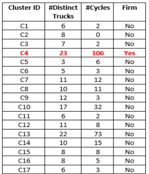
locations to discover the firm for each carrier. A modified DBSCAN algorithm is proposed

to achieve this task by automatically determining the two input parameters based on the

data points provided. Various statistical measures like count of unique trucks and count

of truck visits are applied on the resulting clusters to identify the firms of the respective

carriers. In the second step, we tackle the problem of classifying the stop locations into

two types: primary stops, where goods are transferred, and secondary stops like rest

sta-tions, where vehicle and driver needs are met. This problem is solved using one of the

trade indicator called Specialization Index. Moreover, several set of features are explored

to build the classification model to classify the type of stop locations. In the third step,

having identified the firm, primary and secondary locations, an automated path finder is

developed to identify the truck tours starting from each firm. The results of the

specializa-tion index and the feature-based classificaspecializa-tion in identifying stop events are compared with

the entropy index from previous work. Experimental results show that the proposed set of

cluster features significantly add classification power to our model giving 98.79% accuracy

(6)

DEDICATION

(7)

ACKNOWLEDGMENT

First and foremost, praises and thanks to the God, the Almighty, for His showers of

bless-ings throughout my research work to complete the research successfully.

I would like to reflect on the people who have supported me and helped me throughout

this period of my research. I would like to express my deep and sincere gratitude to my

re-search advisors Dr. Jessica Chen and Dr. Mehdi Kargar for providing invaluable guidance,

continuous support and motivation.

I would also like to thank my thesis committee members Dr. Hanna Maoh and Dr. Pooya

Moradian Zadeh for their valuable guidance, comments and suggestions that added more

value to my thesis work.

I would especially like to deeply thank Dr. Mina Maleki. As my teacher and mentor,

she has taught me more than I could ever give her credit for here. I would like to thank my

mentors Dr. Hanna Maoh and Dr. Mina Maleki from my research at Cross-Border Institute

(CBI) for giving me the opportunity to be a part of this institute for my thesis work.

Also I would like to thank all the staff of Graduate Society of Computer Science for their

kindness. I am extending my thanks to all my friends and colleagues who supported and

helped me during this period.

On a personal note, I would like to express my deepest gratitude to my parents for their

(8)

LIST OF TABLES

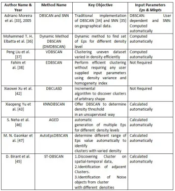
3.1 Summary on DBSCAN Enhancements . . . 41

4.1 An example of information from raw GPS data . . . 50

4.2 An example of processed GPS data . . . 52

5.1 Sample training data for point-based classification . . . 64

5.2 Sample training data for cluster-based classification . . . 65

5.3 Firm information for sample carrier 1 . . . 65

5.4 Firm information for sample carrier 2 . . . 66

5.5 Firm information for 14 sample carriers . . . 66

5.6 Table showing accuracy and error values for SI between 0.09 and 0.20 . . . 69

5.7 Effect on the stop classification with varied cluster radius . . . 71

5.8 Accuracy results for varied cluster radius . . . 72

5.9 Performance of the model over the specialization index and its combination with the cluster features . . . 74

5.10 Performance of the model over the entropy index and its combination with the cluster features . . . 75

5.11 Performance of the model over the combination of SI, EI, and CF . . . 75

5.12 Performance of the model over the formulated index and its combination with the cluster features . . . 76

5.13 Performance of the model over the formulated index and its combination with the cluster features . . . 77

5.14 Feature ranking based on the correlation values of the Features . . . 78

5.15 Sample 1 - Effect of varied cluster radius on the stop classification . . . 82

5.16 Sample 2 - Effect of varied cluster radius on the stop classification . . . 83

5.17 Combined Samples - Effect of varied cluster radius on the stop classification 84 5.18 Sample 1 - Effect of varying Minpts on the stop classification . . . 85

5.19 Sample 2 - Effect of varying Minpts on the stop classification . . . 86

5.20 Combined Sample - Effect of varying Minpts on the stop classification . . . 87

5.21 Performance of the model over the specialization index and its combination with the cluster and temporal features . . . 88

5.22 Performance of the model over the entropy index and its combination with the cluster and temporal features . . . 89

5.23 Performance of the model over the formulated index and its combination with the cluster and temporal features . . . 89

5.24 Performance of the model over the cluster features . . . 90

(11)

LIST OF FIGURES

1.1 Tour . . . 5

2.1 GPS [1] . . . 9

2.2 DBSCAN [2] . . . 16

2.3 Traditional DBSCAN algorithm . . . 17

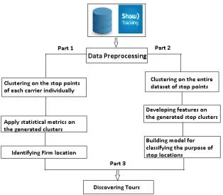
4.1 Overview of Proposed Method . . . 49

4.2 Distance based dwell time calculation [3] . . . 52

4.3 Pseudocode of proposed DBSCAN algorithm to identify firm cluster . . . . 54

4.4 Pseudocode of Modified DBSCAN for finding stop clusters . . . 60

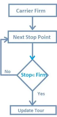
4.5 Workflow of SQL script for finding Tour . . . 62

5.1 Sample stop points . . . 64

5.2 Sample Regions . . . 64

5.3 Specialization Index threshold for classifying Stop locations . . . 67

5.4 Count of Actual Primary and Secondary stops for all SI values . . . 68

5.5 Table and Chart showing Specialization threshold with least error value . . 70

5.6 Charts showing percentage of error for defined SI threshold . . . 71

5.7 Error rate for varied cluster radius . . . 72

5.8 Correlation graph of the features . . . 79

5.9 Relationship between Specialization Index and Unique carrier count . . . . 80

5.10 Relationship between Total Trucks, Unique carrier count and Stop Type . . 80

5.11 Relationship between Specialization Index, cluster features and Stop Type . 81 5.12 Correlation graph of Temporal Features . . . 82

5.13 Sample 1 - Accuracy graph with varied cluster radius . . . 83

5.14 Sample 2 - Accuracy graph with varied cluster radius . . . 84

5.15 Combined Samples - Accuracy graph with varied cluster radius . . . 85

5.16 Sample 1 - Accuracy graph with varied Minpts . . . 86

5.17 Sample 2 - Accuracy graph with varied Minpts . . . 87

5.18 Combined Sample - Accuracy graph with varied Minpts . . . 88

5.19 GPS pings of three trucks for a sample carrier showing Firm . . . 93

5.20 Three Sample Tours of a truck . . . 94

5.21 Sample Tour 1 . . . 95

5.22 Sample Tour2 . . . 96

(12)

LIST OF SYMBOLS

Symbol Definition

GDP Gross Domestic Product

GPS Global Positioning system

DBSCAN Density Based Spatial Clustering Of Applications With Noise

STING Statistical Information Grid

CLIQUE Clustering in QUest

SVM Support Vector Machine

UTC Universal Transverse Mercator

TOA Time Of Arrival

CDMA Code Division Multiple Access

SQL Structured Query Language

SNN Shared Nearest Neighbor

OPTICS Ordering points to identify the clustering structure

CLARANS Clustering Large Applications Based On Randomized Search

SI Specialization Index

EI Entropy Index

FI Formulated Index

CF Cluster Features

(13)

Chapter 1 INTRODUCTION

1.1 Motivation

Major roads and highways constitute the primary transportation infrastructure for the transit

movement of goods. The historical trend of highway investment has taken into account the

role of trucking as the predominant mode of transport. Trucking accounts for 31% of

rev-enue in Canada’s commercial transportation sector by gross domestic product (GDP). The

remaining modes including air-based, rail-based, and marine based travel represent 12%,

11%, and 2% of Canada’s commercial transportation GDP, respectively [4]. By volume,

72% of domestic goods are transported by trucks, while rail and marine modes only haul

21% and 7%, respectively [5]. Major link between Canada and U.S. for freight

transporta-tion on highways are the three border crossing locatransporta-tions i.e. Ambassador Bridge, Peace

Bridge, and Blue Water Bridge. Moreover, trade between Canada and the U.S. relies

heav-ily on trucks as the dominant method of transport. Therefore, domestic and Canada-U.S.

trade are both highly dependent on trucks as a major source of commercial transportation

to ship goods.

One of the technology used in transportation to gain useful information about the

nav-igation and truck tracking is Global Positioning System (GPS). GPS is one such satellite

based technology that helps in tracking of vehicles in real-time. Sensors in trucks and other

freight vehicles also give real-time information about how the vehicle is performing, how

fast it is going, how long it is on the go, how long it is standing still etc. This real-time

data obtained from GPS sensors could be processed and mined to get meaningful

(14)

transportation data from GPS sources usually involves the handling of Big Data. Big Data

in transportation research plays an important role in the information retrieval within freight

transportation. Mining freight information from GPS data using concepts and techniques

in computer science and spatial science highly motivated the present research work.

The continuous growth of the usage of GPS (Global Positioning System) devices in

transportation management systems has evolved into generation of huge amounts of GPS

pings. The enormous spatio-temporal data produced by such devices has greatly increased

the interest in the application of big data mining algorithms. Extracting meaningful

infor-mation from raw GPS data is a crucial task in most location-aware applications. Hence, this

task is becoming more and more interesting. A lot of recent research has focused on

mo-bile phones data, while the commercial vehicles sector is almost unexplored. The problems

typically involve detection of interesting places and classification of the detected locations.

This thesis focuses on one of the major tasks of mining the GPS data coming from the

commercial fleet transportation systems to identify firms for each carrier that are

associ-ated with truck stop locations and then discover the tours starting from each firm. Also,

this thesis includes major contribution in proposing a different approach of categorizing

stop locations using an economic geography index known as the specialization index [6]

and the feature-based classification technique. The proposed approach presented in this

research deals with a combined approach of using clustering and classification techniques.

Clustering technique is basically used for solving two tasks in this research. The first task

involves finding firm location by clustering the stop points of each carrier or fleet

individ-ually. A firm is an establishment of an industry hub that produces the goods that needs

to be transported. Hence, a firm location is unique to each carrier and so we process the

stop points of each carrier individually for finding firm location. Information on the

lo-cations of individual firms can be obtained from commercial organizations like Google or

(15)

freight transportation research. The second task involves the use of clustering technique to

cluster all the stop points and then applying statistical metric to classify the purpose of each

stop location. The data used in this thesis are collected by Shaw Tracking and provided to

us by the Cross-Border Institute at the University of Windsor. The obtained dataset

con-tains individual GPS pings for a large group of Canadian-owned freight carriers with truck

movements across Canada and the U.S. This thesis uses the observed GPS records for the

month of March, 2016. Here, a total of 569 carriers with 40,650 individual trucks with

approximately 75 million GPS pings (i.e. data points) are analyzed. Each GPS ping results

in a data record containing the carrier ID (CID), truck ID (PID), latitude, longitude, and

time. The elapsed time between GPS pings and a dwell time that accumulates if the truck

is stopped can be derived from the input GPS data. Pings associated with meaningful dwell

times represent stop events that can be classified as (1) primary, which occurs when goods

are transferred between the truck and location (or another truck), or (2) secondary, which

occurs when a truck is stationary for other purposes like driver breaks or fuel refills [3].

Identification of the purpose of truck stops is important in mining meaningful information

out of the truck GPS data. Primary stops are particularly important for models since they

denote trip ends for a given truck. The firm is important to be discovered accurately as it

denotes tour ends for a given truck. Likewise, secondary stops are useful since they

com-plement primary stops by providing a complete picture on the nature of truck movements

over space. Hence, it is really important to make accurate distinction between the types of

stops since they correspond to different activities.

The truck tours discovered from GPS trajectory in this research help in building activity

based freight models that represent the microscopic movement of commercial trucks [8].

These micro-simulation models helps traffic engineers and planners simulate freight

activi-ties as part of long-range urban and regional planning exercises. However, the development

(16)

infor-mation needed includes the length of the tours (i.e. duration), the frequency of the stops

made by each truck, as well as the type of the stops (i.e. primary stop for picking or

deliv-ering goods, or secondary stops for resting and/or refueling).

1.2 Research Objective & Solution Outline

This research outlines the identification of the tours accomplishing the shipping of goods

across Canada and US. This broader problem is solved by dividing it into three task: finding

a firm location for each carrier, classifying the stop locations into primary and secondary

stops, and forming the tours that typically starts from a firm location making multiple stops

and return to the same firm location.

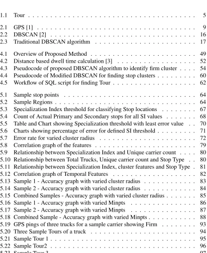
A truck tour is ideally defined as a round trip where a truck starts from the depot or

establishment to perform one or more stops including primary stops for transferring goods

and secondary stops for taking rest or fuel refilling and return to the same initial depot. It

is also called trip chaining in terms of transportation as shown in Fig 1.1.

The objective of this thesis is to mine a large set of truck GPS data using the techniques

of clustering and classification mainly to solve two major tasks. The first task involves

applying clustering technique to the stop points of each carrier individually and identify

the firm location specific to each carrier. The second major task involves categorizing the

stop locations into primary and secondary stops using statistical metric called specialization

index and feature-based classification technique. The classification results obtained from

the proposed method in this thesis are compared with the one using the entropy index [3]

from previous work. The Entropy Index is a measure of the level of order or disorder a

system has. Typically, a system with a high level of order is said to have a low entropy. On

the other hand, higher levels of disorder will be associated with higher entropy. The work

(17)

Figure 1.1: Tour

heterogeneity (i.e. disorder) at a given location. The general idea in [3] is to be able to

determine if a location has a homogeneous cluster in which trucks pertaining to only one

carrier are found at the location. On the contrary, if a location has a heterogeneous cluster

then it will be associated with trucks from a variety of carriers, which makes it more likely

to be a secondary stop. Experimental results show that the feature-based classification

significantly outperforms the latter. The accuracy results showing the comparison with the

entropy index are reported in chapter 5.

1.3 Structure of thesis

The remainder of this thesis is organized as follows.

Chapter 2 presents a brief introduction to GPS Architecture and its basics, together with

an overview of clustering techniques and several clustering models. One of the famous

clustering technique named DBSCAN and its algorithm is also introduced in this chapter.

(18)

Chapter 3 briefly describes previous studies in the field of mining GPS transportation

data to find out meaningful information such as deriving stop locations from the raw GPS

pings, and categorizing of the stop locations. Also, DBSCAN and its variations for finding

clusters with varied shape, size and density, and other similar approaches are summarized.

Several works including the variety of classification features for stop categorization are also

included in this chapter.

Chapter 4 presents the primary contribution of this thesis and describes the

implementa-tion details of our approach. The major contribuimplementa-tion of this research are the following:

• Implementing DBSCAN with automatic calculation of Eps (cluster radius)

parameter.

• Implementing Specialization Index for classifying the purpose of stop

loca-tions.

• Implementing novel stop cluster features and building classification model.

Finally, Chapter 5 reports and discusses the experimental results.

Chapter 6 provides the summary to conclude the thesis along with the directions of

(19)

Chapter 2 BACKGROUND STUDY

2.1 Global Positioning System

The Global Positioning System (GPS) is a satellite-based navigation system that consists of

24-orbiting satellites, each of which makes two circuits around the earth at every 24 hours

[9]. GPS project was developed in 1973 to overcome the limitations of previous navigation

system. GPS was developed and introduced by U.S DEPARTMENT OF DEFENSE and

made freely accessible to everyone [9]. It is also known as NAVSTAR GPS (Navigation

Satellite Timing and Ranging Global Positioning System).

2.1.1 GPS Overview & Architecture

The GPS system provides accurate, continuous, worldwide, three-dimensional position

and velocity information to users with the appropriate receiving equipment. It also

dis-seminates a form of Coordinated Universal Time (UTC) [9]. The satellite constellation

nominally consists of 24 satellites arranged in 6 orbital planes with 4 satellites per plane. A

worldwide ground control/monitoring network monitors the health and status of the

satel-lites. This network also uploads navigation and other data to the satelsatel-lites. The system

utilizes the concept of one-way time of arrival (TOA) ranging. Satellite transmissions are

referenced to highly accurate atomic frequency standards on-board the satellites, which

are in synchronism with a GPS time base. The satellites broadcast ranging codes and

navigation data on two frequencies using a technique called code division multiple access

(20)

MHz) and L2 (1,227.6 MHz) [9]. Each satellite transmits on these frequencies, but with

different ranging codes than those employed by other satellites. These codes were selected

because they have low cross-correlation properties with respect to one another. Each

satel-lite generates a short code referred to as the course/acquisition or C/A code and a long

code denoted as the precision or P(Y) code. The navigation data provides the means for

the receiver to determine the location of the satellite at the time of signal transmission,

whereas the ranging code enables the user’s receiver to determine the transit (i.e.,

propa-gation) time of the signal and thereby determine the satellite-to-user range. This technique

requires that the user receiver also contain a clock. Utilizing this technique to measure the

receiver’s three-dimensional location requires that TOA ranging measurements be made

by satellites. If the receiver clock were synchronized with the satellite clocks, only three

range measurements would be required. However, a crystal clock is usually employed in

navigation receivers to minimize the cost, complexity, and size of the receiver. Thus, four

measurements are required to determine user latitude, longitude, height, and receiver clock

offset from internal system time.

GPS architecture is comprised of three segments:

• Space segment - The space segment consists of a nominal constellation of 24

operating satellites that transmits one-way signals that gives the current GPS

satellite position and time.

• Control segment - The control segment is composed of a master control station,

a network of monitor stations which upload the clock and orbit errors, as well

as the navigation data message to the GPS satellites.

• User segment - User segment consists of the GPS receiver equipment, which

receives the signals from GPS satellites and uses the three dimensional position

(21)

2.1.2 Working of GPS

Figure 2.1: GPS [1]

GPS satellites are orbiting above the earth at an altitude of 11,000 miles. The orbits and

position of satellites are known in advance. These satellites transmit 3-bits of information

to the GPS receiver which includes Satellite number, Satellite position in space and Time at

which the information is sent. Mostly, four nearest GPS satellites send information to the

GPS receiver. GPS satellites uses the method of Trilateration [10] to find out the receivers

position. Data from a single satellite narrows position down to a large area of the earth’s

(22)

spheres overlap. Adding data from third satellite provides relatively accurate position. Data

from fourth satellite enhances precision and also the ability to determine accurate elevation.

A GPS receiver is composed of an Antenna, a Receiver processor, a highly stable clock

and a display for showing location and speed information. GPS Receiver performs the

following tasks.

• Selecting one or more satellites

• Acquiring GPS signals

• Measuring and tracking

• Recovering navigation data

2.1.3 GPS Services & Applications

GPS provides two types of service:

• Civilian Service

• Military Service

The civilian service is freely available to all users on a continuous worldwide basis. The

military service is available to U.S and allied armed forces as well as approved government

agencies.

GPS comes with a vast range of applications:

• Safety cameras

• Scientific experiments

(23)

• Entertainment

• Outdoor activities

The most important applications of GPS are positioning and navigation. GPS tracking

takes the normal functions of a GPS device a step further, by capturing and storing position

data in the internal memory for later retrieval or by transmitting the location data in real

time via the cellular data networks used by mobile phones. A vehicle can be tracked if it

has a GPS device in it. The location information is sent by the GPS device via cell tower

to mobile phone. GPS data is displayed in different message formats over a serial

inter-face. All GPS receivers generally output NMEA data. The NMEA standard is formatted in

lines of data called sentences [11]. Each sentence contains various bits of data organized in

comma delimited format. The GPS data contains information showing the time stamp,

lati-tude, longilati-tude, number of satellite seen and the altitude for each ping in comma delimited

format. The outstanding performance of GPS over many years has earned the confidence

of millions of users worldwide. It has proven its dependability in the past and promises to

be beneficial to users throughout the world in future.

2.2 Clustering

Clustering is the task of grouping a set of objects in such a way that objects in the same

group are more similar to each other than those in other groups [12] . These groups of

similar objects formed are known as clusters. Clustering is a main task of exploratory

data mining, and a common technique for statistical data analysis, used in many fields,

including machine learning, pattern recognition, image analysis, information retrieval,

bio-informatics, data compression, and computer graphics. Popular notions of clusters include

(24)

inter-vals or particular statistical distributions. The appropriate clustering algorithm and

param-eter settings (including paramparam-eters such as the distance function to use, a density threshold

or the number of expected clusters) depend on the individual data set and intended use of

the results. Cluster analysis is not an automatic task, but an iterative process of knowledge

discovery or interactive multi-objective optimization that involves trial and error. It is

of-ten necessary to perform data preprocessing and modify model parameters until the result

achieves the desired properties.

Different cluster models have been developed and for each of these cluster models,

dif-ferent algorithms can be given. The notion of a cluster, as found by difdif-ferent algorithms,

varies significantly in its properties. Understanding these cluster models is key to

under-stand the differences between the various algorithms. Here we explain some major cluster

models.

2.2.1 Grid-based Algorithms

The grid-based clustering approach differs from the conventional clustering algorithms

in a way that it is concerned not with the data points but with the value space that surrounds

the data points. This is the approach in which we quantize space into a finite number of cells

that form a grid structure on which all of the operations for clustering is performed. So,

having a set of records and we want to cluster the data with respect to some attributes, we

divide the related space (plane) into a grid structure and find the clusters [13]. In general, a

typical grid-based clustering algorithm consists of the following five basic steps [14] :

• Creating the grid structure, i.e., partitioning the data space into a finite number

of cells

• Calculating the cell density for each cell

(25)

• Identifying cluster centers

• Traversal of neighbor cells

The following are some techniques that are used to perform Grid-Based Clustering:

• CLIQUE (CLustering In QUest)

• STING (STatistical Information Grid)

• WaveCluster

STING is used for performing clustering on spatial data. Spatial data may be thought

of as features located on or referenced to the Earth’s surface. Its main benefit is that it

processes many common region oriented queries on a set of points efficiently [15]. It

clusters the records that are in a spatial table in terms of location. Placement of a record in

a grid cell is completely determined by its physical location. The spatial area is divided into

rectangular cells (Using latitude and longitude). Each cell forms a hierarchical structure.

This means that each cell at a higher level is further partitioned into smaller cells in the

lower level. The computational complexity is O(k) where k is the number of grid cells at

the lowest level. Usually k<< N, where N is the number of records. STING is a query

independent approach, since statistical information exists independently of queries.

CLIQUE is a density and grid based subspace clustering algorithm that discovers the

clusters by taking density threshold and number of grids as input parameters. CLIQUE

operates on multidimensional data not by operating all the dimensions at once but by

pro-cessing a single dimension at first step and then grows upward to the higher one [16]. It

could generate overlapping clusters within a subspace with one data point belonging to

more than one cluster.

WaveCluster is a novel clustering approach based on wavelet transforms which uses

mul-tiresolution property of wavelet transforms to effectively identify arbitrary shape clusters

(26)

2.2.2 Centroid-based Algorithms

In centroid-based clustering [12] , clusters are represented by a central vector, which

may not necessarily be a member of the data set. Basically, the similarity of two clusters

is defined as the similarity of their centroids. One of the famous centroid based clustering

algorithm is K-means algorithm.

K-means clustering aims at partitioning n observations into k clusters in which each

observation belongs to the cluster with the nearest mean, serving as a prototype of the

cluster. The inputs to the algorithm are the number of clusters and the data set. The data

set is a collection of features for each data point. The number of clusters K can either

be randomly generated or randomly selected from the data set. The algorithm works as a

two-step approach and it iterates between these two steps.

• Data assignment step: Firstly, based on the user input of the number of clusters

K, the algorithm will place K centroids c1, ..,ckat random locations. Each data

point is then assigned to its nearest centroid, based on the squared Euclidean

distance.

• Centroid update step: In this step, the centroids are recomputed. This is done

by taking the mean of all data points assigned to that centroid’s cluster and

this mean point in the cluster will become a new centroid. Based on the new

centroid recomputed, again check all points to see which cluster they are near

to based on Euclidean distance and assign the points to the nearest cluster.

The algorithm iterates between steps one and two until a stopping criteria is met i.e. no

data points change clusters, the sum of the distances is minimized, or some maximum

num-ber of iterations is reached. The k-means algorithm is known to have a time complexity of

(27)

of clusters k to be specified in advance, which is considered to be one of the biggest

draw-backs of these algorithms. Also it does not work well with clusters of different size and

different density, and it fails to detect outliers since it considers all the data points to form

a cluster.

2.2.3 Density-based Algorithms

In density-based clustering, clusters are defined as areas of higher density than the

re-mainder of the data set. Objects in the sparse areas that require separate clusters are usually

considered to be noise and border points.

The most popular density based clustering method is DBSCAN. Density-based spatial

clustering of applications with noise (DBSCAN) [18] is a data clustering algorithm

pro-posed by Martin Ester, Hans-Peter Kriegel, Jrg Sander and Xiaowei Xu in 1996. Given a

set of points in some space, it groups together points that are closely packed together (points

with many nearby neighbors), marking as outliers those points in low-density regions.

The DBSCAN algorithm basically requires 2 parameters:

• Eps: the minimum distance between two points. It means that if the distance

between two points is lower than or equal to this value (eps), these points are

considered neighbors. In other words, it defines the radius n of neighborhood

around a point p.

• MinPoints: the minimum number of neighbors with eps radius to form a dense

region. For example, if we set the minPoints parameter to be 5, we need at least

5 points to form a cluster.

Consider a set of points in some space to be clustered. For the purpose of DBSCAN

clustering, the points are classified as core points, density reachable points and outliers, as

(28)

Figure 2.2: DBSCAN [2]

• A point p is a core point if at least minPts points are within eps distance (eps

is the maximum radius of the neighborhood from p) of it (including p). Those

points are said to be directly reachable from p.

• A point q is directly reachable from p if point q is within distance from point

p and p must be a core point.

• A point q is reachable from p if there is a path p1, .., pnwith p1 = p and pn= q,

where each pi+1 is directly reachable from pi(all the points on the path must

be core points, with the possible exception of q).

• All points not reachable from any other point are outliers.

Pseudo-code of DBSCAN Algorithm

Abstract DBSCAN Algorithm is described below:

• Find the (eps) neighbors of every point, and identify the core points with more

(29)

Figure 2.3: Traditional DBSCAN algorithm

• Find the connected components of core points on the neighbor graph, ignoring

all non-core points

• Assign each non-core point to a nearby cluster if the cluster is an (eps)

neigh-bor, otherwise assign it to noise

DBSCAN visits each point of the database, possibly multiple times (e.g., as candidates

to different clusters). For practical considerations, however, the time complexity is mostly

governed by the number of invocations to the distance calculation function. DBSCAN

executes exactly one such query for each point, and if an indexing structure is used that

(30)

log n) is obtained.

Advantages of DBSCAN

• Does not require a-priori specification of the number of clusters

• Able to identify noise data while clustering

• Able to find clusters of arbitrarily sizes and arbitrarily shapes

Disadvantages of DBSCAN

• DBSCAN algorithm fails in case of varying density clusters

• If the data and the scale are not well understood, choosing a meaningful

dis-tance threshold eps and minpts can be difficult

Applications of Clustering

• Medicine, Computational biology and bio-informatics: Medical imaging,

Hu-man genetic clustering, Sequence analysis

• Business and marketing: Market research that includes market segmentation,

Product positioning and customer surveys

• World wide web: Social network analysis and Search result grouping

• Computer science: Image segmentation, Recommendation systems, Anomaly

detection, Natural language processing

(31)

2.3 Classification

Classification is a process of categorizing where objects are recognized and differentiated

into the set of categories. In machine learning and statistics, supervised classification is a

learning problem of identifying to which of a set of categories a new observation belongs,

on the basis of a training set of data containing observations whose category membership

is known. Some of the well-known examples of classification algorithms include:

• Logistic Regression: It measures the relationship between a dependent

vari-able and one or more independent varivari-ables by estimating probabilities using

a logistic function. The model itself simply models probability of output in

terms of input and it can be used to make a classifier, for instance by choosing

a cut-off value and classifying inputs with probability greater than the cut-off

as one class, below the cutoff as the other [20]. Logistic regression is used in

various fields, including machine learning, most medical fields, and social

sci-ences. Logistic regression may be used to predict the risk of developing a given

disease (e.g. diabetes; coronary heart disease), based on observed

characteris-tics of the patient. The technique can also be used in engineering, especially

for predicting the probability of failure of a given process, system or product.

It is also used in marketing applications such as prediction of a customer’s

propensity to purchase a product.

• Naive Bayes classifier: Naive Bayes is a classification technique based on

Bayes Theorem with an assumption of independence among predictors [21].

In probability theory and statistics, Bayes theorem describes the probability of

an event, based on prior knowledge of conditions that might be related to the

event. In simple terms, a Naive Bayes classifier assumes that the presence of

a particular feature in a class is unrelated to the presence of any other feature.

(32)

features, all of these properties independently contribute to the probability [21].

It works well in many real-world situations such as document classification and

spam filtering. It is easy to build and particularly useful for very large data sets.

• Support vector machines: Support vector machine is a representation of the

training data as points in space separated into categories by a clear gap that

is as wide as possible. New examples are then mapped into that same space

and predicted to belong to a category based on which side of the gap they fall.

It is effective in high dimensional spaces. It uses a subset of training points

in the decision function so it is also memory efficient. In the case of support

vector machines, a data point is viewed as a p-dimensional vector (a list of

numbers), and we want to know whether we can separate such points with a

(p-1) dimensional hyperplane. This is called a linear classifier. There are many

hyperplanes that might classify the data. One reasonable choice as the best

hyperplane is the one that represents the largest separation, or margin, between

the two classes. So we choose the hyperplane so that the distance from it to the

nearest data point on each side is maximized. Intuitively, a good separation is

achieved by the hyperplane that has the largest distance to the nearest

training-data point of any class (so-called functional margin), since in general the larger

the margin, the lower the generalization error of the classifier.

• Random forest: Random forest classifier is a meta-estimator that fits a

num-ber of decision trees on various sub-samples of datasets and uses average to

improve the predictive accuracy of the model and controls over-fitting. The

sub-sample size is always the same as the original input sample size but the

samples are drawn with replacement. This classifier works better in reducing

over-fitting and it is more accurate than decision trees in most cases.

(33)

classi-fication algorithm. It takes a bunch of labeled points and uses them to learn

how to label other points. To label a new point, it looks at the labeled closest

points or the nearest k neighbors to that new point and has those neighbors

vote, so whichever label the most of the neighbors have is the label for the new

point [21]. This algorithm is simple to implement, robust to noisy training data,

(34)

Chapter 3 LITERATURE REVIEW

This chapter gives a brief overview of the research work carried out for processing GPS

data and mining useful information from it. GPS technology is widely used in trucking

companies for the purpose of fleet tracking. GPS data obtained from these trucking

com-panies are in form of raw pings which basically includes details like Carrier ID, Truck ID,

Latitude and Longitude Points and Time of each ping. To mine useful information out of

these raw GPS pings, involves the usage of Big Data in freight transportation. A lot of

research has been done in this area to process this GPS data and other useful information

involved in freight transportation.

In this section, we briefly introduce different clustering techniques used to extract

activ-ity stops. Various types of clustering methods have been developed and different techniques

are used as per different application needs. Moreover, which clustering techniques to select

highly depends on the nature of the dataset. DBSCAN is the most popular among all

den-sity based clustering algorithms for geographical spatial data. Different versions and

mod-ifications to DBSCAN have been implemented to find activity stop locations. Moreover,

graph based clustering is also widely used to discover trajectory clusters. In the following,

we discuss related work used to find activity locations with different approaches.

3.1 Related works on the identification of stop locations

Extraction of stop locations in GPS trajectory is one of the most popular problem in mining

geographical data. Previous studies covers variety of methods to deal with the stop

identi-fication task. To accomplish this task, two general approaches were used: static approach

(35)

lo-cations that could possibly be the stop lolo-cations are predefined. So when extracting stops

from trajectories, if a vehicle enters into a predefined location and the stay duration exceeds

the duration threshold, this previously defined region is regarded as a stop location in the

trajectory. The main drawback of static algorithms is that users need to specify their

respec-tive places of interest. As a result, this approach will fail to discover some of the additional

and unknown interesting locations if they are not provided by users beforehand. Also this

approach is quite difficult to apply on big datasets including millions of GPS records as it

is not practical to define and cover all the important locations for the complete dataset.

In the dynamic approach, the user does not need to have a prior knowledge regarding

the stop locations. Several classical clustering algorithms are introduced to extract stops

from a trajectory under this approach. Considering only the spatial characteristics of the

trajectory data, previous work has included the implementation of clustering techniques

such as variation of traditional K-Means method [24] in order to detect stop locations. The

selection of the value of parameter K and the initial clustering center is the main drawback

because it heavily affects the results. Modified DBSCAN algorithm named DJ-Cluster

(density and join-based clustering algorithm) [25], is proposed to detect personal

mean-ingful places. These density-based clustering algorithms only take spatial dimensions into

consideration and the temporal sequential features are ignored. Several studies have also

considered temporal information along with the spatial one. Different DBSCAN

enhance-ments with temporal sequential characteristic have been considered, and adopted by many

researchers in order to extract stop positions [25–29]. An improved DBSCAN algorithm

with gap treatment was proposed in [26] to detect stop episodes in a trajectory. The

CB-SMoT (clustering-based stops and moves of trajectories) [27] algorithm was proposed to

extract known and unknown stops where clusters are generated by evaluating trajectory

sample points at a slower speed than the velocity threshold. In addition to the velocity

(36)

pro-posed in [28] improves the CB-SMoT algorithm by proposing an alternative for calculating

the Eps parameter, but it is still difficult to calculate as it depends on users to distinguish the

low speed part and high speed part. Additionally, by assigning different thresholds to

dif-ferent characteristics, some clustering approaches have been proposed [1821]. A two-step

clustering technique to discover most frequently visited locations from the GPS trajectory

data is introduced in the TDBC (a spatio-temporal clustering method used to extract stop

points from individual trajectory) algorithm [21]. Additionally, a time-based clustering

al-gorithm [30] was proposed considering both the clustering distance threshold and the time

threshold.

Lei Gong et al. [31] used a two-step method for identifying activity stop locations. In the

first step, modified version of DBSCAN algorithm is used to identify stop points and move

points. In the second step, one of the machine learning algorithm called support vector

ma-chines (SVMs) method is used to distinguish between activity stops and non-activity stops

from the identified stop points. Improved DBSCAN algorithm, named C-DBSCAN, is

in-troduced in this paper. This improved algorithm works with two constraints that basically

takes into account the time sequence constraint and a direction change constraint. These

constraints are used to avoid errors due to moving points or points representing movement

along a straight road at low speed. The first constraint says that all points in a cluster

should be temporally sequential. So if the points are separated in a sudden, the cluster will

be divided into two clusters at the point of sudden increase of distance and each one will

be tested to see if it satisfies the condition of minimum number of points in one cluster.

The second constraint says that the percentage of abnormal points in a cluster should not

exceed a given threshold value. Pseudocode for C-DBSCAN algorithm is explained in

de-tail. It requires five input parameters i.e. Trajectory data (T), neighborhood of core points

(eps), minimum number of points in a cluster (Minpts), threshold percentage of abnormal

(37)

moving points. In the second step, once the stop points and moving points are discovered,

SVM is used to classify between activity and non-activity stops considering features like

stop duration, mean distance to the centroid of a cluster of points at a stop location. This

proposed algorithm was applied on GPS data collected using mobile phones in the Nagoya

area of Japan in 2008. Experimental results were carried out to compare the results of the

proposed algorithm with the traditional one with respect to four different indexes as

de-scribed in the paper. Improved DBSCAN algorithm (C-DBSCAN) achieves an accuracy

of 90% in identifying stop locations and the SVMs method is almost 96% accurate in

dis-tinguishing activity stops from non-activity stops. One of the drawback of this approach

is that the dataset used in this paper does not include traffic congestion, hence it may be

considered as an activity stop and current methods and attributes used in SVMs may not

handle it well.

Zhongliang Fu et al. [30] proposed a two-step clustering technique to discover most

frequently visited locations from the GPS trajectory data. In the first step, they extract

stop points using spatio-temporal clustering algorithm based on time and distance. The

second step involves applying improved clustering algorithm based on a fast search and

identification of density peaks to discover the trajectory locations. Pseudocode of the novel

spatio-temporal clustering technique based on time and distance, which is abbreviated to

TDBC, is presented in this paper. The algorithm takes single trajectory T, time threshold dt

and distance threshold dd as input conditions. It finds clusters which represent stop points.

Furthermore, it also uses a function that checks the relationship between the current cluster

and the previous cluster and process the cluster either by merging them or considering a

new stop point based on this function check. In the second step, improved Clustering by

Fast Search is applied to the discovered stop points to extract trajectory locations based

on density peak. Steps has been explained in the paper to find the density peaks for

(38)

data collection application installed in the smart phones by 30 volunteers. Three different

datasets were tested for the number of stop points found for different distance and time

thresholds and presented as graph representation in this paper. The proposed TDBC was

compared with the other four algorithms, K-Medoids, DJ-Cluster [25], CB-SMoT [27] and

Time-Based Clustering [32]. Summary table of the results obtained from these algorithms

is represented with respect to time complexity, precision and recall. Results from the table

shows that k-medoids, DJ-Cluster and CB-SMoT are more time-consuming than the other

two algorithms due to their complex computation. The efficiency of the TDBC is similar to

the Time-Based and both have high clustering efficiency. In terms of precision, the TDBC

and DJ-Cluster are over 0.8, which is significantly larger than the other three algorithms.

In terms of recall, compared with the others, the TDBC is slightly improved. However, the

proposed approach requires some prior parameters, and manual intervention is necessary

when the cluster centers are selected.

W. Chen et al. [33] proposed a modified density-based clustering algorithm, named

T-DBSCAN, by considering the time sequential characteristics of the GPS points along a

trajectory. Three formal terms called Trajectory, Stop, and Move used in T-DBSCAN are

defined below:

A trajectory is the user-defined record of the evolution of the position of an object that is

moving in space during a given time interval in order to reach a given destination.

trajectory: [tbegin, tend]−>space

A stop is a part of a trajectory, such that (1) The user has explicitly defined this part

to represent a stop, (2) The temporal extent [tbeginstopx, tendstopx] of this part is a

non-empty time interval, and (3) The traveling object does not move, i.e. the spatial range of the

trajectory for the interval is a single point. (4) All stops are temporally disjoint, i.e. their

temporal extents are always disjoint.

(39)

represent either two consecutive stops, or tbegin and the first stop, or the last stop and tend,

or tbegin and tend. (2) The temporal extent [tbeginmovex, tendmovex] is a non-empty time

interval, and (3) The spatial range of the trajectory for interval [tbeginmovex, tendmovex]

is a spatiotemporal polyline defined by the trajectory function.

Four input parameters are required for T-DBSCAN: D is the set of points comprising the

trajectory; Eps is an inner radius for identifying density-based neighborhood; CE ps is an

outer radius for limiting the density searching range; Eps is the search radius; and MinPts

is the minimum number of neighboring points to identify a core point. Pseudocode of

T-DBSCAN algorithm has been defined in this paper. Two tests were performed to provide

a comparative analysis between DBSCAN and T-DBSCAN in terms of segmentation

ac-curacy and computation efficiency. First test indicated that T-DBSCAN was significantly

faster than DBSCAN in segmenting the trajectories at all data levels. Specifically,

TDB-SCAN took only 6.25% of DBTDB-SCAN’s time to process up to 8000 points, and this ratio

decreased to 5.72% and further 4.34% when 8000˜20000 points and 20000˜30000 points

were processed, respectively. The second test involved comparison of accuracy between

the two methods. Compared to the real stops from field verification, all T-DBSCAN

de-duced clusters had correct match except those clusters that resulted from a traffic jam. In

comparison, serious overlapping occurred between many pairs of clusters identified with

DBSCAN.

Benoit Thierry et al. [34] proposed a novel kernel-based activity location detection

al-gorithm in comparison with the classical detection method based on distance and time

thresholds [35], [36], [37]. This novel algorithm detects (i) known activity locations and

(ii) time spent at a given location, depending on algorithm bandwidth value, GPS noise

level and actual stop duration. Kernel density estimation is a non-parametric method where

a symmetrical kernel function is first superimposed over each event. The set of

(40)

frequently used for point pattern analysis and hotspot exploration. The proposed algorithm

runs globally by calculating a kernel density surface [38] instead of grouping spatially

nearby points. This creates a smoothed surface corresponding to the probability density

function of 2D points. This smoothed surface is controlled by the bandwidth. The peaks of

this surface determines the candidates for actual stops. Explanation of this kernel-density

algorithm (Akd) and of the classical fixed threshold algorithm (Aft) are presented in this

paper. Experiments were conducted on randomly generated GPS tracks and results show

that the proposed algorithm outperforms the fixed threshold algorithm for almost all

indi-cators, correctly identifying the three artificially generated stops with varying duration and

noise levels. Similarly, although Aft had the best spatial accuracy with smaller bandwidths

and for the lowest noise levels, Akd succeeded in maintaining a better overall accuracy

across all bandwidths and noise categories.

All the techniques seen so far in the related work, need to consider reasonable threshold

values for both the distance and time parameter. Also, while calculating the density of GPS

points, most clustering-based algorithms take the number of GPS points within a given

distance into account, without considering their sequential characteristics. The concept of

move ability [39] is introduced where the density of GPS points will be calculated using

the adjacent points over the trajectory, not the overall spatial points. In [39], Kun Fu et al.

introduced a novel approach of move-ability and hybrid feature based density clustering

which considers temporal and spatial properties to find stop points in GPS trajectory data.

Various definitions are described in this paper for defining the concept of move-ability and

a formula for calculating it. In the first step, move-ability is calculated for each points in

the trajectory. Basically, stop points in a trajectory should have lower move-ability and

higher density of GPS points. Hence in the second step, an improved DBSCAN is applied

which calculates density to define a core point. Experiments were conducted on Geolife

(41)

a sequence of temporal, ordered, time-stamped points; each point contains geographical

coordinate information, such as longitude, latitude and altitude. To validate the proposed

technique, results were compared to four other stop-detection algorithms: the CB-SMoT

algorithm [27], DBSCAN algorithm, DJ-Cluster algorithm [25], and time-based clustering

[32]. Results show that this novel approach is more robust to fake stops which occurs due

to congestion owing the concept of move-ability.

Kevin Gingerich et al. [3] applied an alternative approach where both the distance and

time measures were used, also considering the sequential characteristics of GPS pings for

identifying stop locations. So, in order to find the truck stop locations, the GPS pings for

a given truck is sorted sequentially according to the registered time stamp and the location

of a first ping is compared to the location of the next ping. If the distance between two

consecutive pings is less than a certain distance threshold, the dwell time is set equal to the

elapsed time between the two pings. If the distance of the third ping from the first ping is

also less than the threshold value, the dwell time continues to accumulate. The elapsed time

of all these pings will keep on adding up to dwell time until there is a ping located outside

the buffer threshold distance at which point the dwell time is reset. A reasonable distance

threshold with radius of 250 m was selected in a way to avoid cutting a stop short if a vehicle

moved a limited range within a given property and also to avoid the spatial errors that might

arise due to bad GPS readings. To investigate the potential of false positives in the data,

an area containing Highway 401 road links between Highway 407 and Highway 403/410

in Ontario, Canada (latitude between 43.588 and 43.638; longitude between -79.819 and

-79.661) was considered. This area was selected since it has the largest concentration of

GPS pings in the dataset and occurs along a heavily congested highway corridor in the

Toronto metropolitan area in Ontario. Only 48 out of 32,174 stop events in the examined

area are false positive stop events suggesting that the potential for obtaining erroneous

(42)

All the previous study considered most of the characteristics of geographical data such

as distance threshold, time threshold, direction change, adjacent sequential data, and group

of whole data for clustering to extract stop points from the GPS data points. Also, the novel

approach of move ability applied in [39] shows good results in finding out stop locations.

Other works considering distance and time measures in [3] along with the entropy concept

to process real-time individual truck pings in sequential manner with the distance and time

threshold parameter also generated quite good results and were validated manually to check

its correctness. This approach is proved feasible for large volume of data by evaluating the

pattern that emerges from analyzing stop events over space. Hence, we apply the same

technique to process the GPS data points carrying the same nature of the dataset.

3.2 Related works on the variations and enhancements of the clustering

techniques

Clustering techniques considering varied shape, size and density of the clusters

Adriano Moreira et al. [40] described implementation of two density based clustering

algorithms: DBSCAN [41] and SNN [42] to identify clusters from geographical data based

on their spatial density to characterize geographic regions. This paper mainly introduces

working of DBSCAN and SNN algorithm which also includes discussion on how the

val-ues for the input parameters to be selected for these algorithms. These algorithms were

implemented in Visual Basic 6.0. It also compares the cluster results obtained from both

algorithms. Although DBSCAN can find clusters with different shape and size, it fails to

find clusters with different density. On the other hand, SNN algorithm can find clusters of

different densities. Two different approaches of the SNN algorithms were implemented.

The first approach is a Core Approach. It creates the clusters around the core points. The

second approach is a Graph Approach in which clusters are identified by the points that

(43)

similar-ity is higher than the Eps value. The results obtained through the use of these algorithms

show that SNN performs better than DBSCAN since it can detect clusters with different

densities while DBSCAN cannot. The only drawback here is that both the density based

algorithms require two parameters Eps and MinPts to be inputted manually and the cluster

results changes greatly with the change in the parameter values inputted to the algorithm.

Mohammed T. H. Elbatta et al. [43] proposed an enhancement of DBSCAN algorithm

called Dynamic Method DBSCAN (DMDBSCAN) that has the ability to detect the clusters

of different shapes, sizes that differ in local density. DMDBSCAN uses dynamic method

to find suitable value of Eps for different density level in the data set instead of using global

Eps value. Distance from point is calculated to its kth nearest neighbor, which is defined as

k-dist. These k-dists are computed for all data points for some k value inputted by user, and

a graph is plotted for this value of k-dists sorted in ascending order. The sharp curve in the

graph corresponds to suitable value of Eps for each density level of data set. Lastly,

DB-SCAN is applied for each Eps value to find the clusters with different density. Experiments

were conducted on three artificial two-dimensional data sets as well as three real dataset

and results obtained using proposed approach were compared with traditional DBSCAN

and DVBSCAN with different parameter values. Also, a table showing the results across

average error index and the number of generated clusters for each algorithm is presented in

this paper. Results show that the proposed algorithm DMDBSCAN gives more stable

esti-mates of the number of clusters than existing DBSCAN or DVBSCAN over many different

types of data of different shapes and sizes.

Peng Liu et al. [44] implemented new variation of DBSCAN algorithm called

VDB-SCAN to get clusters from varied-density data. The basic idea of this algorithm is to

de-termine different values of eps parameter for different density of the data points instead of

single global eps value as used in traditional DBSCAN for the purpose of generating varied

(44)

to look at the behavior of the distance from a point to its kth nearest neighbor, which is

called k-dist. The k-dists are computed for all the data points for some k, sorted in

ascend-ing order, and then plotted usascend-ing the sorted values. As a result, a sharp change is expected

to see. The sharp change at the value of k-dist corresponds to a suitable value of Eps. This

value of Eps that is determined in this way depends on k, but does not change

dramati-cally as k changes. VDBSCAN is implemented with 2 steps. In the first step, VDBSCAN

calculates and stores k-dist for each point and partition k-dist plots. The number of

den-sities is determined by k-dist plot so it selects Epsi parameter value for each density. In

the second step, DBSCAN algorithm runs for each Epsi(i=1,2,3,...,n. n is the number of

density levels). Epsihave been ordered as k-dist line curves, that is Epsi<Epsi+1 (i<n).

Before performing DBSCAN for Epsi+1, it marks the points in clusters corresponding with

Epsi as Ci - t (t is a natural number), which indicates that the points belong to the cluster

t in density level i. Marked points will not be processed by DBSCAN again. Non-marked

points after all the Epsi process are recognized as outliers. The experimental results show

that VDBSCAN generates different clusters with different density, while it takes the same

time complexity as DBSCAN.

EDBSCAN (An Enhanced Density Based Spatial Clustering of Application with Noise)

algorithm [45] is another extension of DBSCAN which clusters the data points with varying

densities effectively. It keeps tracks of density variation which exists within the cluster. It

calculates the density variance of a core object with respect to its -neighborhood. If the

density variance of a core object is less than or equal to a threshold value and also satisfying

the homogeneity index with respect to its neighborhood, then it will allow the core object

for expansion. It calculates the density variance and homogeneity index locally in the Eps

neighborhood of a core object. Steps for the proposed algorithm are described in detail.

The idea is to use varied values for Eps according to the local density of the starting point

Big Data Mining to Construct Truck Tours

Scholarship at UWindsor

Scholarship at UWindsor

Big Data Mining to Construct Truck Tours

Big Data Mining to Construct Truck Tours

Big Data Mining to Construct Truck Tours

DECLARATION OF ORIGINALITY

ABSTRACT

DEDICATION

ACKNOWLEDGMENT

TABLE OF CONTENTS

LIST OF TABLES

LIST OF FIGURES

LIST OF SYMBOLS

Chapter 1

INTRODUCTION

1.1

Motivation

1.2

Research Objective & Solution Outline

1.3

Structure of thesis

Chapter 2

BACKGROUND STUDY

2.1

Global Positioning System

2.2

Clustering

2.3

Classification

Chapter 3

LITERATURE REVIEW

3.1

Related works on the identification of stop locations

3.2

Related works on the variations and enhancements of the clustering

techniques