LI, WEIFU. Design of Hardware Accelerators for Hierarchical Temporal Memory and Convolutional Neural Network (Under the direction of Dr. Paul D Franzon).
In recent years, the artificial neural network (ANN) achieved incredible successes in
numerous application areas. Among these ANNs, hierarchical temporal memory (HTM) and
convolutional neural network (CNN) has been considered as one of most representative networks
in the cortical learning algorithm and machine learning algorithm respectively. In this paper, we
propose a multi-level hierarchical ASIC implementation to support full-scale HTM and an ASIP
implementation of CNN to leverage the zero input features and weights in convolutional layers.
To improve the unbalanced workload in HTM, the propose design provides different mapping
methods for the spatial and temporal pooling respectively. Also, we implement a distributed
memory system to improve the efficiency of memory bandwidth. Finally, the hot-spot operations
are optimized using a series of customized units. Regarding to scalability, we propose a ring-based
network consisting of multiple processor cores to support a larger HTM network. To evaluate the
performance of our proposed design, we map an HTM network that includes 2048 columns and
65536 cells on both the proposed design and NVIDIA Tesla K40c GPU using the KTH database
as input. The latency and power of the proposed design is 6.04ms and 4.1W using GF 65nm
technology. Compared to equivalent GPU implementation, the latency and power is improved
12.4x and 70.2x respectively. For CNN, the proposed ASIP can support a novel dataflow for the
1-D primitive that allows us to skip the computations with zero input features and weights by
processing the data encoded in run-length compression (RLC) format directly. For computations
beyond 1-D primitives, the proposed ASIP can perform multiple 1-D primitives in parallel, all of
which share the input feature row but with various weight rows. By dividing an array of 96 PEs
proposed design can achieve a frame rate of 56.6f/s for the AlexNet at 1.65W, and a frame rate of
2.6f/s for the VGG16 at 1.58W. Compared to Eyeriss, the proposed design provides a 2.0x and
4.65x processing latency improvement for AlexNet and VGG16 respectively with the similar
© Copyright 2019 by Weifu Li
Network
by Weifu Li
A dissertation or submitted to the Graduate Faculty of North Carolina State University
in partial fulfillment of the requirements for the degree of
Doctor of Philosophy
Electrical Engineering
Raleigh, North Carolina 2019
APPROVED BY:
_______________________________ _______________________________ Paul D. Franzon James Tuck
Committee Chair
ii
DEDICATION
iii
BIOGRAPHY
Weifu Li was born in June 1987, Harbin, China. He received his bachelor’s degree from
Harbin Institute of Technology in July 2010, and his master’s degree from Northeastern University
in Dec 2012. In January 2013, he started his graduate research work with Dr. Paul D. Franzon in
the area of digital hardware design in North Carolina State University. His major research interests
include the custom accelerator design for machine learning algorithms.
iv
ACKNOWLEDGMENTS
Most of all, I would like to thank my wife, Zijian Chen, for her unconditional support, love
and understanding all these years. I will never be able to achieve this without her encouragement.
I also want to thank my parents for their endless love during my entire life.
I want to express my sincere gratitude to my research advisor, Dr. Paul Franzon, for his
guideline, understanding and support. I also want to thank him for introducing me to the machine
learning related research topic and providing me the opportunity to join the research areas that are
changing the our world. In addition, I want to thank my committee member, Dr. James Tuck, Dr.
David Ricketts and Dr. Xipeng Shen for insightful advice and understanding during the research
work.
I would like to thank my colleagues in NCSU, Steve Lipa, Lee Baker, Josh Schabel, Sumon
Dey, Josh Stevens, Zachary Johnston and Tse-Han Pan for their help, advice and support on the
physical design follows.
Finally, I would like to express my endless love to my kids Kyrie and Kyle, you are the
v
TABLE OF CONTENTS
LIST OF TABLES ... vi
LIST OF FIGURES ... vii
Chapter 1: Introduction ... 1
1.1. Motivation ... 1
1.2. Contribution ... 3
1.3. Organization ... 5
1.4. Abbreviations ... 6
Chapter 2: Background ... 8
2.1. Fundamental of HTM ... 8
2.1.1. Spatial Pooling ... 10
2.1.2. Temporal Pooling... 12
2.2. Fundamental of CNN ... 14
Chapter 3: State-of-the-art... 18
3.1. HTM Implementation ... 18
3.2. CNN Implementation ... 20
Chapter 4: Design of HTM Accelerator... 24
4.1. Overview of Hardware Accelerator ... 24
4.2. Network Mapping&Implementation ... 29
4.2.1. Spatial Pooling ... 29
4.2.2. Temporal Pooling... 32
4.2.3. Inter-Core Communication ... 36
4.3. Functionality Validation and Performance Evaluation ... 38
4.3.1. Network Configuration ... 38
4.3.2. Verification Dataset ... 39
4.3.3. Functionality Validation ... 40
4.3.4. Performance Evaluation ... 44
4.4. Conclusion ... 48
Chapter 5: Design of CNN Accelerator ... 49
5.1. Zero-Skipping Technology ... 49
5.1.1. Existing Challenges ... 49
5.1.2. Proposed Solutions... 52
5.2. Proposed Dataflow ... 57
5.3. Design of Proposed Hardware ... 65
5.3.1. Central Processor ... 66
5.3.2. Processing Element ... 68
5.3.3. Network-on-Chip ... 70
5.3.4. Customized Instruction ... 73
5.4. Performance Evaluation ... 76
5.4.1. Sensitivity to Network Density ... 76
5.4.2. Design Specification ... 81
5.4.3. Benchmark Performance ... 83
Chapter 6: Conclusion and Future Work ... 88
6.1. Conclusion ... 88
vi
LIST OF TABLES
Table 2.1 Information in PE Controller Memory ... 26
Table 2.2 Information Stored For Each Column ... 27
Table 2.3 Information Stored For Each Distal Synapse ... 27
Table 2.4 Configuration of Target Network ... 39
Table 2.5 Test One of First Order Network ... 40
Table 2.6 Test Two of First Order Network ... 41
Table 2.7 Test One of High Order Network ... 43
Table 2.8 Noise Test of High Order Network ... 44
Table 2.9 Performance Comparison with GPU Baseline ... 45
Table 2.10 Post-Route Power and Area of the Proposed Design ... 46
Table 2.11 Performance Comparison with State-of-the-arts ... 48
Table 5.1 PE Utilization Rate of AlexNet ... 61
Table 5.2 Configuration Instructions in Proposed Design ... 73
Table 5.3 Details of Port Configuration Instructions ... 74
Table 5.4 Processing Instructions in Proposed Design ... 74
Table 5.5 DRAM Access Instructions ... 75
Table 5.6 Performance Summary of Cooperation and Parallel Mode ... 80
Table 5.7 Specification of the Proposed Design ... 81
Table 5.8 Performance Summary of Convolutional Layers in AlexNet ... 84
vii
LIST OF FIGURES
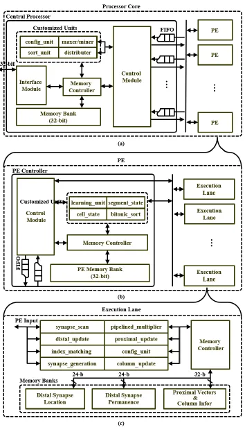
Figure 4.1 (a) Schematic of Processor Core (b) Schematic of PE (c) Schematic of
Execution Lane. ... 25
Figure 4.2 Mapping Example of Spatial Pooling... 30
Figure 4.3 Implementation of Global Inhibition In Proposed Design ... 31
Figure 4.4 Mapping Example of Temporal Pooling. ... 33
Figure 4.5 Example of Index Matching for One Segment. ... 35
Figure 4.6 Example of Proposed Ring Network. ... 37
Figure 4.7 Examples of Images from KTH Database ... 39
Figure 4.8 Processing Latency vs Percentage of Existing Segments... 47
Figure 5.1 Example of 1-D Primitive with a Stride of One ... 50
Figure 5.2 (a) 1-D Primitive without Any Zero-Skip Technology. (b) 1-D Primitive with Skipping Zero Input Features. (c) 1-D Primitive with Skipping Zero Input Features and Weights ... 51
Figure 5.3 Example of Input Row in RLC format ... 52
Figure 5.4 Bits per Word vs Data Sparsity. ... 53
Figure 5.5 Example of Vertical Processing Sequence. ... 55
Figure 5.6 Example of Weight Row in RLC Format. ... 56
Figure 5.7 Example of Input Feature Row Reuse Using 3 x 3 Filter... 59
Figure 5.8 Example of Processing Within One PE Group... 60
Figure 5.9 Example of Processing with Weight Exchange... 60
Figure 5.10 (a) Schedule of Processing Passes for “conv2-1” in VGG16 without Weight Exchange. (b) Schedule of Processing Passes for “conv2-1” in VGG16 with Weight Exchange. ... 64
Figure 5.11 Schematic of Proposed Processor Core. ... 65
Figure 5.12 Schematic of Modulo/Divider Unit. ... 67
Figure 5.13 Schematic of Proposed Processing Element... 68
Figure 5.14 Example of PE Grouping and Port Configuration. ... 72
Figure 5.15 Normalized Cycler Per vs. Network Density of 7x7 Filter ... 77
Figure 5.16 Normalized Cycler Per vs. Network Density of 5x5 Filter ... 78
viii
1
CHAPTER 1
INTRODUCTION
Artificial neural networks (ANNs) are biologically inspired system designed to emulate the
way in which the human brain processes information by detecting the patterns and relationships in
data and learn through experience [1]. From the aspect of modeling neocortex, we can divide most
of these ANN-based algorithms into two categories, the machine-learning algorithm (MLA) and
the cortical learning algorithm (CLA). Most MLAs nowadays model each synapse as a continuous
weight value and learn the knowledge through repeatedly updating these weight value during the
training. On the other hand, the CLAs model each synapse as one or multiple binary bits and use
the summation of all bits belonged to one neuron to indicate corresponding status. The CLAs learn
knowledge by generating new synapses or updating the existing ones to emulate the way a human
brain learns. In this work, we focus on one of the most representative algorithms in each category,
the Convolutional Neural Network (CNN) in MLA and Hierarchical Temporal Memory (HTM) in
CLA. Then, we implement an specific integrated circuit (ASIC) and an
application-specific instruction set processor (ASIP) for HTM and CNN respectively to explore the potential
performance improvement from the custom hardware designs.
1.1. Motivation
In the past few years, HTM has been demonstrated as successful in anomaly detection for
identifying unusual changes in network servers [2], and to detecting anomalous data sequences in
the network bus of vehicles [3]. In addition, several applications of HTM, such as geospatial
tracking, nature language predictions and stock volume anomalies is under commercial test [4]. In
2
In the area of pattern recognition, the HTM network in [6] can achieve an accuracy of 95.65% on
traffic sign recognition and HTM network in [7] outperforms several other neural network on
automatic license plate recognition. The integration of HTM on top of a Support Vector Machine
(SVM) achieved a 96% classification rate in an object recognition task [8].
Unlike most neural networks in MLAs, HTM is not a matrix-based network and the data
dataflow within each neural column and cell is un-deterministic. Therefore, though there are large
amount of parallelisms existing at each step of the entire algorithm, the steps in each column and
cell can be various depending on the local input data, column state and cell state, which results in
an unbalanced workload among the processing engines (PEs). Meanwhile, each column and cell
in HTM requires intensive memory accesses, which are narrow, discrete and asynchronous due to
the sparse distributed representation (SDR) of active columns and the workload difference among
columns/cells. Consequently, mapping HTM network onto a conventional hardware platform like
GPU and CPU fails to achieve a satisfactory performance. Fortunately, we efficiently handle these
issues by providing proper design of ASIC-based hardware accelerator. Furthermore, the custom
hardware design allows us to further improve the performance of HTM by optimizing these critical
steps.
Regarding to MLA, CNNs have achieved an unprecedented success across a board range
of applications including the face detection [9], image classification [10], speech recognition [11],
advertisement recommendation [12], and even the game playing [13]. Particularly, CNN achieve
a near-human performance in video [14] and audio recognition [15]. However, given the increasing
complexity of potential applications, the size of state-of-arts CNNs is also dramatically increased.
For instance, AlexNet [16], a state-of-art CNN proposed in 2012, has about 2.3M parameters in
3
15.3M to beat the accuracy of AlexNet with same testbench. For most of these state-of-arts CNNs,
the convolution operation in each layer dominates the total execution time [18] and requires up to
hundreds of megabytes (MB) of parameters for a single pass in inference. Therefore, optimizing
the latency and power of convolutional layers can significantly improve those of entire CNN-based
system.
Though there are many research focusing on optimizing the performance of convolutional
layers by allocating more arithmetic units, increasing the size of on-chip SRAMs and developing
better dataflow, the performance improvement from these methods highly depends on the available
hardware resource and the total number of required computations stays constant. This work tries
to improve the performance of convolutional layers from a different angle and is motivated by the
observation that the immediate convolutional layers can have up to 79% and 89% of zero input
features in AlexNet and VGG16 due to the rectified linear unit layers (ReLUs). Meanwhile, using
the pruning technology proposed in [19] can reduce the average percentage of none-zero weight
down to 36.7% and 32.6% in these CNNs. As a result, skipping operations with zero input features
or zero weights could significantly reduce the total number of computations in the convolutional
layers, which allows us to improve the latency and power of CNNs with same hardware resource
and memory bandwidth.
1.2. Contribution
In this work, we implement a custom ASIC for HTM to explore the performance benefits
from the proposed optimization methods. The details of our contributions for HTM is:
• Design and implement a hierarchical architecture and control flow to improve the unbalanced
workload and synchronization issues among the columns and cells while maintaining the
4
• Design and implement a distributed memory organization, which assigns a dedicated memory
bank to each level of the proposed hierarchy, to improve the utilization efficiency of memory
bandwidth. The simulation results have demonstrated that the proposed design can outperform
the GPU implementation with 8.04x smaller memory bandwidth.
• Design and implement a series of custom hardware modules to improvement the performance
of critical operations in HTM, such as the global inhibition, selecting learning/active cells and
counting distal segment activity.
• Design and implement an ASIC-based accelerator to perform an HTM network including 2048
columns and 65536 cells. Compared to the equivalent implementation on NVIDIA Tesla 40Kc,
the proposed design achieves a 12.45x speedup, 2.15x silicon area deduction and 137x power
efficiency.
For CNN, we implement a custom ASIP that can support various network sizes and the
concrete contributions on this work include,
• Design and implement a novel dataflow for 1-D convolution primitive that allows us to directly
process the data encoded in run-length compression (RLC) format. As a result, the proposed
design can skip the operations with zero input features and weights to improve the processing
latency.
• Design and implement a dataflow beyond 1-D convolution primitive that makes all the PEs in
proposed design share the same input features in parallel and minimize the data movement
between on-chip and off-chi memory.
• Design and implement an ASIP-based hardware accelerator to support the proposed dataflow
and outperform state-of-arts designs with similar hardware resource while benchmarking
5
• Investigate the influence of input feature and weight sparsity, weight filter size and operation
mode on the processing latency in proposed design to achieve the most optimized
performance for various CNNs.
1.3. Organization
We organize the rest of this dissertation as follow. Chapter 2 introduces the fundamentals
of HTM and CNN including the network architecture and operations in both algorithms. In chapter
3, we survey the related state-of-arts design of CNN and HTM on various hardware platforms and
briefly compare them with the proposed design.
Chapter 4 presents the custom ASIC design of HTM. This chapter starts from the overview
of the proposed processor core. Then, we introduce the network mapping method, optimization for
critical operations and design scalability applied to overcome the performance bottleneck in the
existing implementations. In the result section, we describe the functionality validation for both
software and hardware implementations, then discuss the result of their performance comparison
from the aspects of processing latency, silicon area and power consumption.
Chapter 5 presents the proposed zero-skipping technology and corresponding ASIP design
of CNN. We start from the technology introduction applied within each 1-D convolution primitive
that allows us to skip the computations with zero input features and weights. Then, we discuss the
dataflow among multiple 1-D primitives. In subsequence section, we elaborate the design of
ASIP-based processor core. In the result section, we investigate the influence of sparsity and weight filter
size on processing latency and compare the performance of proposed design against the
start-of-art custom hardware implementation.
In Chapter 6, we summarize the design methodology and achieved improvement for both
6
1.4. Abbreviations
ANN Artificial Neural Network
MLA Machine Learning Algorithm
CLA Cortical Learning Algorithm
CNN Convolutional Neural Network
HTM Hierarchical Temporal Memory
DCNN Deep Convolutional Neural Network
DNN Deep Neural Network
ASIC Application-Specific Integrated Circuit
ASIP Application-Specific Instruction Set Processor
SDR Sparse Distributed Representation
CPU Central Processing Unit
GPU Graphics Processing Unit
FPGA Field-Programmable Gate Array
PE Processing Element
DSP Digital Signal Processing
NoC Network-on-Chip
RLC Run Length Compression
MB Mega Bytes
KB Kilo Bytes
eDRAM Enhanced Dynamic Random-Access Memory
SRAM Static Random-Access Memory
7 1/2-D One/Two Dimension
Psum Partial Summation
MAC Multiply and Accumulation Computation
8
CHAPTER 2
BACKGROUND
In this chapter, we describe the fundamental properties of both HTM and CNN including
the network structure, the operations in neurons and the data storage format. Considering the nature
of online learning algorithm, we introduce both learning and inference mode of HTM in the section
2.1. For CNN, we focus on the inference mode since most of applications nowadays can directly
utilize the pre-trained weight filters.
2.1. Fundamental of HTM
HTM is an on-line machine learning algorithm inspired by the structural and algorithmic
properties of neocortex in the human brains [20]. By combining and extending approaches in the
spatial and temporal clustering algorithms and the sparse distributed representation (SDR), HTM
has the capacity to learn and recognize streaming data, and then makes a prediction for the next
possible input data based on the learned knowledge. Meanwhile, we can consider HTM as an
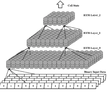
unsupervised learning algorithm since it can learn the unlabeled data. Normally, a typical HTM
network consists of multiple layers organized as a hierarchy, each layer of which shares the same
operations but has different network sizes. In general, HTM network use the binary data received
from the practical world as input data at bottom level, and then recombines the output data from
lower levels at higher layer to memorize a complicated pattern as shown in Figure 2.1. In addition,
HTM has the potential to combine multiple networks together, each of which works on the data
from different resources as shown in Figure 2.2. Jeff Hawkins firstly proposed the HTM algorithm
in his book [21] in 2004. In 2011, Jeff Hawkins and his colleagues published the 2nd generation
9
Figure 2.1A Three-layer HTM Network
10
In general, we can model each layer of HTM network as a 2-D matrix of columns, each of
which contains multiple identical cells. For each input data, HTM network extracts both spatial
and temporal information in the format of column and cell state respectively. During processing,
we can perform HTM algorithm in two operation modes: learning and inference. The inference in
HTM is a process of matching current input pattern with the ones learned. Each input data uses a
list of active columns to represent its spatial pattern, and then turns corresponding cells into active
or predict state to represent the temporal pattern.
In learning mode, HTM performs all operations in inference mode. In addition, operations
used to update parameters related to column activity, such as column boost value and permanence
of proximal synapses, are performed in spatial pooling to create a unique SDR for each input. In
temporal pooling, each learning cell in active columns either generates a series of connections or
updates the strength of existing connections to memorize the temporal pattern of input data.
2.1.1. Spatial Pooling
Motived by how our human brain always represents the outside world information in only
a small percentage of active neurons, the major purpose of spatial pooling is to generate the SDR
for each input pattern in the format of active columns. By using the SDR, we integrate several
desirable properties into HTM network.
1) In HTM, we can represent the complicated input patterns, in which most input bits are
active, by only a small percentage of columns without losing any information. Since
many operations in HTM are only performed in active columns, the memory space,
processing time, and power consumption for single input pattern can be improved over
11
2) Generally, input data received from the practical world is always accompanied with
various noise. Since flipping just a few bits in the input data might not affect the SDR
generated by the spatial pooling at all, HTM is more robust to deal with input data
containing spatial noise or missing parts.
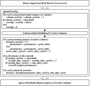
Spatial Pooling
Binary Input from Real Word or Lower Level
Sparse Distributed Representation of Activity Columns For each connected proximal synapses in columns:
column_activity = column_activity + 1 If column_activity >= threshold: overlap = Activity × Boost else,
overlap = 0
Column Global Inhibition2% Active Columns
For each proximal synapses in active columns: If input_vector[i] == 1:
permanence = permanence + perm_delta else:
permanence = permanence - perm_delta active_duty_cycle(i) = active_duty_cycle(i) + 1
For all columns in the network: If column_activity >= threshold:
overlap_duty_cycle(i) = overlap_duty_cycle(i) + 1 If overlap_duty_cycle(i) >= min_duty_cycle: reset all synapse permanence
For each column in network:
boost[i] = boostfunction(active_duty_cycle(i), min_duty_cycle)
Figure 2.3Operation Details of Spatial Pooling
In spatial pooling, each proximal synapse in all the columns randomly connect to 1 bit of
corresponding binary input vector. In cast that a proximal synapse is connected to an input bit of “1” and has a permanence value above the threshold, we consider it as a “connected synapse” and
we use the summation of connected synapses in a column as column activity as shown in
Figire.2.3. The operations in dot block only perform under learning mode. During global
inhibition, we sort all columns within the same region in descending order of overlap value. Then
12
combination of active columns as output of spatial pooling. In learning mode, it increases the boost
value of columns that are less active to increase its possibility of being active for next input data.
Meanwhile, the synapse permanence value increases if it connects to a “1”. Otherwise, the value
decreases.
2.1.2. Temporal Pooling
In temporal pooling, HTM combines the output from the spatial pooling, stored as an SDR,
and the previous cell state at t-1 to generate the temporal representation of each input, which is the
combination of active cells at t. The details of temporal pooling are described in Figure 2.4 The
definition of several of the terms used in describing HTM are as follow,
1) Distal synapse: the connection between any two cells from different columns refers to
the distal synapse and a synapse is considered as “connected” if its permanence value
is above threshold.
2) Distal segment: a group of distal synapses within the same cell connected to cells from
same or similar combinations of active columns is distal segments.
3) Segment activity: the total number of connected synapses to active/learning cells at t
refers as the segment activity of active/learning cells at t.
4) Best matching cell: a cell has largest number of synapses to active cells at t -1 or fewest
number of existing segments in a column is the best matching cell.
In inference mode, cells in each active column are turned into active state if they were at
predict state at t-1. In case that there is not any predict cells at t-1, all cells in that active column
are turned into active state to indicate an unexpected input data. To make a prediction for the next
input, we turn a cell into predict state if its maximum segment activity of active cells at t is above
13
In learning mode, for each active column, we turn a cell into learning state if it was at
predict state at t-1 and has a segment activity of learning cells at t-1 above threshold. Otherwise, we select the “best matching cell” as learning cell. In each learning cell, we generate a new segment
if the largest segment activity of active cells at t-1 is below threshold. Otherwise, we increase the
permanence value of synapse connected to active cell at t-1 and decrease that of all the other
synapses in the segment with largest activity. In addition, if a cell was in predict state for the past
two input data but never turns into learning state, the permanence value of all connected synapses marked in prediction phase is decreased to reduce “incorrect” predictions.
Temporal Pooling
Column State
Active and Predict State of Cells For each cell in one active column:
If cell[i]. predict[t-1] == true and segment_activity(active, t-1) >= Threshold: active_cell_find = true
cell[i].active[t] = true If active_cell_find == false: cell[i:0]. active[t] = true
For each cell in one active column:
If active_cell_find == true and segment_activity(learn, t-1) >= Threshold: learn_cell_find = true
cell[i].learn[t] = true If learn_cell_find == false:
cell[best_matching_cell]. learn[t] = true
generate new segment or mark connected synapses in active segment
For each cell in one column:
If cell[i].segment_activity(active, t) >= Threshold: cell[i].predict[t] = true
mark all connected synapse in active segment
For each cell in one column: If cell[i].learn[t] == true:
increase permanence of all marked connected synapses
decrease permanence of all marked unconnected synapses else if cell[i].predict[t : t-1] == false:
decrease permanence of all marked connected synapses
14
Though spatial pooling can generate different SDR for each input, temporal pooling allows
HTM network to memorize the input data as an ordered sequence rather than a sequence of
non-related data. In addition, temporal information is necessary for distinguishing identical input data at different locations in the same sequence. Taking the input sequences “a, b, d, b, e” as an example,
both letter “b” in spatial pooling should have the same combination of active columns due to the
identical input vectors as shown in Figure 2.5 (a). During the temporal pooling, since HTM use
both column state and cell state at t-1 as input data, the combination of active cells at t can be various following different precedents. Since the precedents of two “b” are different in this
sequence, the combinations of active cells at t is also different as shown in Figure 2.5 (b), where
the blue indicates the active cells for the first “b” and the red ones are for the second one.
(a)
(b)
Figure 2.5(a) Combination of active columns for letter "b". (b) Combination of active cells for letter “b”
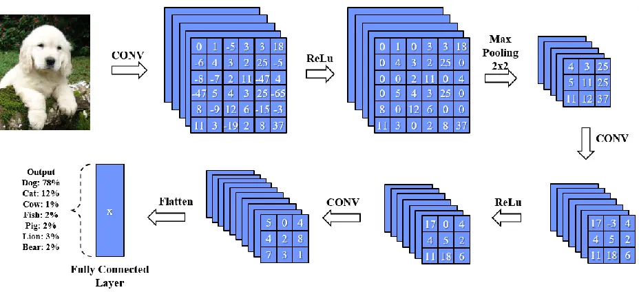
2.2. Fundamental of CNN
CNN is a class of supervised matrix-based machine learning algorithm and usually consists
of multiple computation layers including convolutional layer, max-pooling layer, non-linear layer
and the fully connected layer as shown in Figure 2.6. The state-of-art CNNs nowadays can have a
total layer number up to 192. By sweeping multiple weight filters across the entire input data, the
15
the format of feature maps, referred as output features. Then, we can downsize the output features
of by performing max pooling, which only leaves the maximum value within a pooling window.
The non-linear layers in CNNs are used to increase the network non-linearity, so that adding more
layers can provide a better approximation power. The most successful non-linear function for CNN
is the Rectified Non-Linear unit (ReLU), which force all the negative values in the output features
to zero. Compared the other non-linear functions, the ReLU can speed up the training progress and
increase the overall sparsity. The same group of convolutional layers, max-pooling layers and the
ReLU can be repeated multiple times to extract the high-level feature for each input data. Finally,
we flat the output features and use them as the input of the fully connected layers for classification.
Though there can be several fully connected layers, the neuron number of the final fully connected
layer should equal to the category number of target dataset. Meanwhile, the output value from each
neuron indicates the possibility of corresponding category.
16
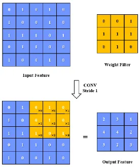
The computation in CNNs mainly come from the high-dimensional convolution operations
between the input features and the corresponding weight filters, each of which can produce one
element of the output feature map. More specifically, it includes the element-wise multiplications
between one filter and corresponding receptive field in the input feature, and the summation of all
these products as shown in Figure 2.7.
Figure 2.7Example of Convolution Operation
Usually, each convolutional layer in CNN consists of multiple weight filters, each of which
includes various channels. During inference, we sweep each channel of a weight filter across the
corresponding channel of target input feature with a given interval, referred as stride, to generate
17
resulted from all channels of a filter to generate one complete output feature. We repeat the same
iteration with all input features and weight filters of a given convolutional layer. Since each output
feature from the previous layer is used as one input channel of the next layer, the filter channel
number of a convolutional layer is usually related to the total filter number of its previous layer. A
processing example between one input feature and one weight filter is shown in Figure 2.8, where the “C” stands for the channel number of target filter.
18
CHAPTER 3
STATE-OF-THE-ART
During the past few years, there has been numerous works about HTM and CNN published
due to their successes in various application areas. In this chapter, we present the state-of-the-art
hardware implementations of both networks including the key features, performance and potential
improvement achieved in our design.
3.1. HTM Implementation
To improve the performance of HTM on the traditional hardware platforms, HTM has been
implemented using multi-core CPU and GPU. However, due to the nature of parallel computation,
intensive memory access and dynamic workload distribution, mapping HTM onto these platforms
fails to achieve a satisfactory performance. In [22], two latency hotpot operations in the sequential
CPU implementation were identified and re-implemented using OpenMP library in parallel. Then,
the author mapped the parallelized code onto the multiple-core processor and evaluated the latency
vs number of cores occupied. Though adding more cores can improve the processing latency, the
parallel efficiency decreases from 100% down to about 48% while the number of cores increases
from 1 to 6. In addition, they predicted the efficiency can deteriorate if using more cores. For the
GPU implementation, we proposed an optimized CUDA-based implementation of HTM on GPU
as our performance baseline. Though the GPU implementation allows us to explore the parallelism
existing at each operation of HTM, it could not improve the unbalanced workload distribution and
memory bandwidth utilization efficiency, which limits the performance improvement from GPU
implementation for large network. This is also demonstrated by the simulation results discussed in
19
Regarding the customized hardware design, Lennard and his team implemented a scalable
hardware accelerator optimizes the memory organization, power and area by leveraging the
large-scale solid-state flash memory in 2016[23]. The proposed design is validated by the MNIST dataset
and achieved a classification accuracy of 91.98%. The power and area of proposed spatial pooler
is 30.538mm2 and 64.394mW respectively under TSMC180nm Technology. In the same year, Abdullah’s group proposed a reconfigurable and scalable architecture of HTM in [24]. They ported
the design for a 100-column matrix onto a Xilinx Virtex-IV FPGA fabric, and then verified it with
both MNIST and EU number plate dataset, which achieved a 91% and 90% accuracy respectively.
In addition, the proposed hardware offers a speedup of 4817x over the software implementation.
Both works, however, only implemented spatial pooling in HTM and cannot explore the temporal
patterns of input data, which is one of most important features of HTM compared to other neural
algorithms.
In [25], we proposed a fully flattened hardware design for the complete HTM algorithm,
in which we mapped each column and its corresponding cells onto one processing element (PE),
and connected all PEs through the mesh network. To verify the proposed design, we implemented
a 400-column PE matrix, each of which can include up to 2 neural cells, to perform a series of test
cases using MNIST dataset. Compared to the software implementation in [22], the proposed design can achieve a speedup of 329.6 with a power and area of 1.29mW and 17511μm2 for single PE. In
[26], Abdullah’s group again presented a FPGA-based design for both spatial pooler and temporal
memory. They developed a synthetic synapse concept to address the dynamic interconnections of
synapses during learning. For a 100-column matrix with 3 cells per column, the proposed design
provides a processing latency of 5.75us for one image in MNIST dataset with a power of 1.39mW
20
network size in their testbench is relatively small compared to the typical one of 2048 columns
[27] and did not discuss about the potential challenges and solution to handle the scalability, which
is extremely important for real-world applications.
In [28] and [29], they proposed two analog implementations of HTM using the memristor
circuits. The [28] implemented the 2-D column array using parallel memristor crossbar arrays and
validated the design on both face recognition and speech recognition dataset. In [29], the authors
implemented a modified version of spatial and temporal pooling using the memristor logic circuits
and demonstrated the propose design with multiple face recognition dataset. Though the analog
implementations allow us to remove the analog-to-digital converter between the input sensor and
processing engineer, these implementations are not configurable and are power and area hungry.
For instance, each image pixel requires a memory cell in [29], which has an area of 23.85um2 and
a power of 0.44mW using the TSMC 0.18um Technology. Therefore, the total power and area of
memory cell only can be huge even processing a small input image. To the best of our knowledge,
the work presented in this paper is the first hardware implementation that can support the both
spatial and temporal pooling with a large network size.
3.2. CNN Implementation
In recent years, there has been numerous papers about custom hardware accelerators aimed
at skipping the computations with zero weights or input features published. For skipping zero input
features, the author of [18] encoded each row of the input features into the run length compression
(RLC) format, which can efficiently reduce the total DRAM accesses for sparsity input features.
It also proposed a dataflow named row stationary to improve the energy efficiency. The proposed
design can achieve a frame rate of 34.7fps with a power of 278mW for AlexNet and a frame rate
21
stored in the on-chip memory in the dense format, it cannot fully eliminate the energy resulted
from moving zero value among on-chip memory banks. In addition, though gating the multiplier
when the zero input features are being processed can save computation energy, it cannot really
improve execution time due to idle cycles in the pipeline arithmetic units. Meanwhile, Eyeriss in
[18] did not skip the operations with zero weights. In [30], the author proposed the DaDianNao[31]
based custom hardware accelerator to skip the computations with zero input features. The proposed
design decoupled the groups of execution lanes in original architecture, which allows each
execution lane to access memory independently to asynchronization among execution lanes. They
encoded the input features stored in eDRAM into the zero-free neuron array format (ZFNAf),
which provides an offset for each none-zero value, to skip the computations with zero input
features. The proposed claimed a latency improvement of 1.38x and 1.39x compared to the original
design. However, the ZFNAf format cannot efficiently skip the zero-related computations while
the whole data bricks are zero and is not capable to handle the zero weights either. In addition, the
proposed data format can result in a significant increase in memory space and memory access
energy regardless the density of input feature.
Regarding skipping zero weights, the proposed design in [32] only stored and none-zero
weights of each neuron, so that the inefficiency computations can be skipped. It also allowed each
PE to access the memory asynchronously to improve the utilization efficiency of PEs. They also
implemented an index module using step indexing method to calculate the index of corresponding
input features for each none-zero weight. The proposed design provided a 7.23x speedup compared
against the DadianNao. However, this work cannot skip the computations with input features and
is less efficiency while processing the convolutional layers compared to that of fully connected
22
[33] proposed an energy efficiency neural processing unit that supports both convolutional layer
and fully connected layer. They integrated 1024 MAC units, which are connected using a bufferfly
structure and divided into two cores. By applying the feature-map selection circuitry, the proposed
design can skip the computations with zero weights. The NPU achieved a 6.9TOPs and 3.5TOPs
for the 5x5 and 3x3 weight filters while there are 75% zero values. The power of proposed design
is 39mW and 1553mW under 0.5V and 0.8V respectively. Though this work can skip zero-weight,
it cannot skip those computations with zero input features. In addition, they did not benchmark the
proposed design with any state-of-the-arts CNNs to evaluate the actual performance.
In [34], the author compressed both input features and weights using a variant of the sparse
matrix representation to reduce memory accesses. They also proposed a novel dataflow named as
PlanarTiled-InputStationary-CartesianProduct (PT-IS-CP), in which each PE reads multiple
none-zero weights and input features within a given region, and then delivers them into a multiplier
array along with their coordinates. Then, it passes all these products into a series of accumulation
buffer to calculate the partial sums. Compared to a dense CNN accelerator, the proposed design
can provide an average latency improvement of 2.37x and 3.52x for the AlexNet and VGGNet
respectively. However, the proposed dataflow assumes a filter stride value equal to 1. Otherwise,
there are many unnecessary none-zero multiplications, since each input feature is only covered by
a part of the filter when the stride is larger than 1. As a result, the efficiency of proposed accelerator
will be decreased while supporting the convolutional layers with a stride value larger than one,
such as AlexNet. In addition, it requires a large SRAM to store the input/output features on-chip
and a high DRAM bandwidth to maintain the performance compared to other designs. In [35], they
23
controller, the proposed design can identify the none-zero operand pairs, so that the inefficient
computations can be skipped. They also proposed zero-aware kernel allocation method to improve
the unbalanced workload resulted from filter sparsity. Overall, the proposed design achieved a
4.4x/5.6x speedup using the pruned AlexNet/VGG16 as input data compared to that of their own
implementation of Eyeriss. However, since the fetch controller still need to scan through the result of all “AND” operations to find the none-zero pairs, it is difficult to keep the pipelined arithmetic
units busy, which can result in a decrease in the computation efficiency. In addition, this proposed
design dose not employ any data compression technology for input features or weights to improve
the memory access energy.
It is also worth to mention that none of these state-of-the-arts provide an absolute latency
per frame as performance metrics except [18], which makes it difficult for us to perform
apple-to-apple comparison.
In addition to paper focusing on sparse convolution layer, there are also some
state-of-the-arts focus on improving performance of hardware accelerator without any zero-aware technology,
such as [36] and [37]. In [36], the author proposed a DCNN processor consisting of multiple DSP
clusters, a co-processor and around 5.6MB on-chip SRAM. The proposed accelerator is fabricated
using 28nm FD-SOI technology and can provide a frame rate of 58frame/s for AlexNet. In [37],
the author presented an energy-scalable processor, which supported the dynamic voltage accuracy
frequency scaling technology to improve the energy efficiency. After quantizing the input features
and weights down to 4-bit, the proposed design can achieve a frame rate of 47frame/s and a power
24
CHAPTER 4
DESIGN OF HTM ACCELERATOR
In this chapter, we present the design details of proposed HTM hardware accelerator, which
includes the architecture overview, network mapping method, operation implementation and the
design scalability. We perform a series of test cases to validate the functionality our hardware and
software implementation and robustness against noise data. In the result section, we compare the
performance of our proposed accelerator with that of equivalent software implementation.
4.1. Overview of Hardware Accelerator
In the proposed design, a processor core is organized as a 2-level hierarchical architecture
as shown in Figure 4.1. The first level of the hierarchy consists of 1 central processor and 8 PEs,
each of which connects to the central processor through two 32-bit data ports and two 2-bit control
ports. The second level of hierarchy exists in each PE and consists of 1 PE controller and 8 identical
execution lanes.
The central processor consists of four parts, a control module, a series of customized units,
an interface module and an on-chip memory bank as shown in Figure 4.1 (a). The control module
is responsible for system configuration, synchronizing the PEs and collecting data from all PEs.
Coordinated by the control module, the customized design units can perform operations requiring
data from all PEs, such as the global inhibition, without any inter-PE communication. The interface
module is designed to implement the inter-core data communication described in the later section.
The memory bank in central processor stores packages received from other processor cores or local
25
26
Similar to the central processor, there is a control module in each PE controller designed
to implement the inter-lane data communication and synchronize all execution lanes as shown in
Figure 4.1 (b). Each PE controller includes a series of customized units used to perform the
operations requiring data from all execution lanes, such as counting distal segment activity. The
memory bank in PE controller is used to store information for local cells, such as existing segment
number per cell, cell states, and the list of active/learning cells. We summarize the information
stored in PE memory bank in Table 2.1. The lists of active/learning cells at t and t-1 in each
processor core can have up to 40 elements, since each processor core can support up to 2048
columns and only 2% of the total column should become active for each input data.
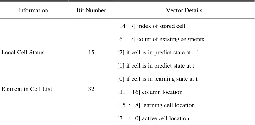
Table 2.1Information in PE Controller Memory
Information Bit Number Vector Details
Local Cell Status 15
[14 : 7] index of stored cell [6 : 3] count of existing segments [2] if cell is in predict state at t-1 [1] if cell is in predict state at t [0] if cell is in learning state at t Element in Cell List 32 [31 : 16] column location
[15 : 8] learning cell location [7 : 0] active cell location
The primitive module in our proposed design, referred as the execution lane, implements
27
Each execution lane includes multiple individual custom units as shown in Figure 4.1 (c), each of
which implements one specific operation in the spatial and temporal pooling. Each execution lane
has a dedicated memory bank used to store the information of proximal and distal synapses mapped
on local PE. In case that all memory space for the distal synapses is occupied, the newly generated
synapses will overwrite the existing ones. The details of stored information for one column and
one distal synapse is summarized in Table 2.2 and 2.3 respectively.
Table 2.2Information Stored For Each Column
Information Bit Number Per Vector Vector Number Per Column
Synapse Mapping Vector 32 2
Synapse Status Vector 32 2
Synapse Permanence 32 40
Column Value Vector 48 1
Each word for the columns is 32-bit.
Table 2.3Information Stored For Each Distal Synapse
Information Bit Number Per Vector Vector Details
Synapse Index Vector 24
[23 : 8] location of connected column [7 : 0] location of connected cell Synapse Permanence 16 [15 : 0] permanence value of distal
synapse
Synapse Status Vector 8
28
Each bit in synapse mapping vector indicates the connection status between one synapse
and 1-bit data in input vector, while the corresponding bit in synapse status vector indicates if that
synapse is active based on the current permanence value. The column value vector records column
boost value and times of being active for each column. HTM network only requires and updates
the column information during spatial pooling and update them after the processing of each input
in learning mode.
The data format for each distal synapse includes two kinds of vector, location of connected
cells (X and Y index) and corresponding connection strength referred as permanence value. The
lower 4-bit of each synapse status vector records information such as, if it is a valid synapse, and
if the synapse is just generated during the learning of current input.
Instead of putting one large and wide memory in the central processor, we distribute the
memory across each level of the proposed hierarchical design. Compared to a centralized memory
system, the distributed one can improve the memory access overhead and power efficiency with a
given bandwidth due to the following reasons,
1) Unlike the matrix-based algorithms, such as convolutional neural network and long
short-term memory, the memory access in HTM is not always continuous, since some
of the operations are only performed in the active columns/cells, which are usually
discretely stored in memory. In addition, the data size of a single column/cell is usually
small (16-32 bits). As a result, the total number of memory access using one 256-bit
memory will be similar as that using eight 32-bit memories while reading this kind of
data. However, due to the higher power and sequential access of that 256-bit memory,
it is more efficient from the aspect of power to use 8 distributed memory banks in HTM
29
2) For operations on the continuously stored data, each access to the centralized memory
can get data for multiple PEs or execution lanes. However, the processing latency of
each PE or execution lane can vary depending on the states of target columns or cells.
For instance, the execution lane for active column requires more cycles to update
proximal synapses than others. As a result, using centralized memory can resulted in
duplicated accesses to same location from different lanes. In the proposed distributed
memory, since each execution lane has a dedicated memory, we can fully eliminate this
situation.
4.2. Network Mapping & Implementation
In the proposed design, the network mapping onto hardware is different in spatial pooling
and temporal pooling. In this section, we will discuss the details of hardware implementation and
network mapping
4.2.1. Spatial Pooling
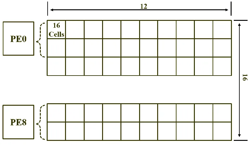
During spatial pooling, the proposed design divides the entire network into multiple
sub-regions of columns, each of which is mapped onto one PE. In Figure 4.2, we present a network
example of spatial pooling, in which a 16x12-column matrix is mapped onto 8 PEs and each PE is
responsible for the computation of a sub-region with 8 x 2 columns. In the practical world, it is
impossible to process all these columns within the same sub-region simultaneously due to the
limitation of hardware resource and memory bandwidth for input data. Therefore, we further divide
the columns mapped on one PE into multiple batches, each of which consists of 8 columns equaling
to the number of execution lanes in each PE. During one iteration, we map each column from the
30
time. The PEs in the proposed design repeat the same iteration until all columns in network are
processed.
In the proposed design, we implement spatial pooling as two individual operations, (1)
computation of the overlap values (2) sorting of the overlap values from all PEs to find the active
columns in inference mode. To compute the overlap value, each execution lane in all PEs reads
both mapping and status vector of the proximal synapses, which are randomly generated and
downloaded into each memory bank during the initial phase. Meanwhile, execution lanes start to accumulate the bitwise “and” operation result of these two vectors and the input vector to calculate
the activity of one column in the “synapse_scan” unit. After processing all vectors connected to
one column, each execution lane multiplies the local column activity by a corresponding boost
value to obtain the overlap value of current column in case that its column activity is larger than
the threshold.
31
For each iteration, there are a total of 64 overlap values from all the PEs. Along with the
value from previous batch, we need to sort 104 overlap value to find the top 40 active columns. In
this work, we divide the entire sorting process in two phases as shown in Figure 4.3. In phase one,
the overlap value in each PE is re-ordered by an 8 element bitonic sorter in the PE controller. Then,
the sorted arrays from all PEs are sent to the central processor at the same time, in which there is
a 4-level pipeline comparator used to find the top 40 columns from all PEs by always moving the
columns with larger overlap values to the next level. Compared to the implementation in [25], the
proposed design only requires 39 comparators, which is 52x fewer. In addition, the max number
of active columns in the proposed design is configurable up to the network size in this work, but
is limited by the number of comparators and buffers in [26].
32
The hierarchical architecture in the proposed design allows us to implement the two-phase
sorting as a pipeline, in which we sort the overlap of the n and n+1 column batches in the PEs and
the central processor simultaneously. Since the sorting performed in PEs is faster than that in the
central processor, we combine the sorting in PEs with the operations used to calculate the overlap
value for one batch. As a result, we re-organize the operations of spatial pooling in inference mode
as a two-state pipeline, which allows us to bury the latency of the faster stages (overlap calculation
+ PE sorting) into the slower one (sorting in central processor) to improve the overall performance
of spatial pooling. In the learning mode, we still perform the operations used to find these active
columns in pipeline, and perform the learning operations after all the columns processed.
In the learning mode, we perform three more operations in the “column_update” unit and
the “proximal_update” unit in all execution lanes and the “column_state” unit in PE controllers to
update the local boost value, times of being active column, and the permanence value of proximal
synapses. Then, each bit in the synapse status vector is re-evaluated based on the latest permanence value, “1” indicates proximal synapse with value above threshold.
4.2.2. Temporal Pooling
Parallelism in temporal pooling exists at both column level and cell level. However, due to
the mechanism of finding active columns in spatial pooling, using the same mapping method in
Figure 4.2 can result in a dynamic distribution of active columns among all the PEs. Since some
operations in temporal pooling are only performed in active columns, the PEs with more active
columns have to suffer a much longer processing latency, while the rest PEs stay idle, which can
eventually result in a significant increase of the total processing latency. In addition, this situation
33
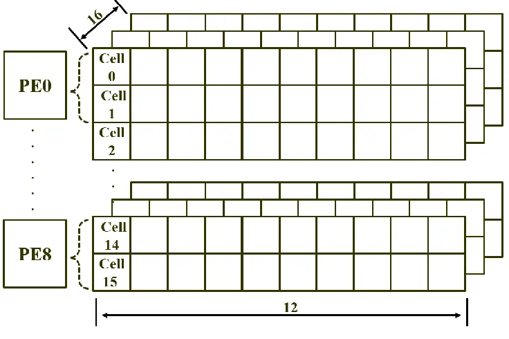
To optimize the unbalanced workload, the proposed design divides cells in the network
into 8 layers, each of which is mapped onto one PE. In Figure 4.4, we present a mapping example
of temporal pooling, where we reuse the same network dimension in spatial pooling. Since there
are 16 cells in each column, each PE in the proposed design is responsible for the computation of
384 cells now. Consequently, the number of active columns mapped onto each PE is always same
regardless of their locations, which can result in a more balanced workload at PE level. In temporal
pooling, most operations target on the distal synapses within certain cells, which can be performed
on all synapses from the same segment in parallel. To exploit this parallelism, the proposed design
evenly distributes all the distal synapses from one segment among all execution lanes within each
PE during temporal pooling. Compared to mapping cells onto the execution lanes, the proposed
synapse-level mapping can significantly improve the unbalanced workload resulted from the
various existing segment number and cell state at execution lane level.
34
The temporal pooling majorly consists of two operations in inference mode, deciding active
cells and deciding predict cells. The state of each cell in both operations depends on the activity of
distal segments and its previous state at t-1. Generally, we obtain the segment activity by checking
the state of cells connected by the target distal synapses and counting those at learning/active state.
However, due to the sparse distribution of connected cells, obtaining segment activity of multiple
cells in parallel requires intensive cross-PE memory accesses, which can result in significant
inter-PE communication overhead.
In the proposed design, we count the target segment activity by counting the number of
matching pairs between the cells in current active list and those stored in target segment. More
specifically, the processing starts from each execution lane reading out one synapse index vector
belonging to the target segment. Then the PE controller begins to broadcast all elements in current
active list to all local execution lanes one by one, while execution lanes are matching the index of
local synapse with the received ones. Since the cell index in both active list and distal synapses is
stored in the descending order of column index, we only need to broadcast the active list one time
for each segment regardless of the synapse number per segment. Once the PE controller broadcasts
all elements in that active list, we can count the activity of target segment by summing the number
of matching pairs in all execution lanes up in the “segment_state” unit located in the PE controller.
An example of index matching for one segment is shown in Figure 4.5. Different from the previous
implementation, execution lanes in the proposed one only accesses the local memory banks, which
can dramatically improve the latency for obtaining one segment activity.
In additional to the network mapping method, the number of existing segments in each PE
can influence the workload as well. In the proposed design, there is a unit named “distributor” in
35
column, the “distributor” collects the maximum segment activity and existing segment number of
learning cell candidates from all PEs and then assigns the learning cell into the PE with the best
matching cell. In case that the cells from multiple PEs have the same segment activity and existing
segments number, the “distributor” unit finds the PE with least total segment through customized comparator name “miner” and assigns the learning cell into that PE to balance the total number of
segments among all PEs.
Figure 4.5Example of Index Matching for One Segment.
In learning mode, there is one more operation to perform to update the permanence value
36
execution lanes. The “cell_state” unit in PE controller loops through the state vectors of all local
cells. In case of finding a “dirty” cell, the PE controller enables “distal_update” unit in all execution
lanes, each of which is responsible for the update of one synapse. Execution lanes repeat the same
operation until all distal synapses in that “dirty” cell are updated. The concrete update value for
each synapse depends on both synapse status vectors in local memory bank and the cell/segment
status received from PE controller.
4.2.3. Inter-Core Communication
The total memory size of one single processor core limits the maximum size of the network
mapped onto it. However, simply increasing the size of memory bank to process a larger network
can result in a dramatic decrease in performance, since we are mapping more columns/cells onto
each PE now. To efficiently process a larger network or improve the performance of a given
network, the proposed design supports a ring-based inter-core network includes multiple identical
processor cores as shown in Figure 4.6. Each core within the network connects to two neighbor
cores through two 32-bits single direction data ports and two 2-bits control ports. The bandwidth
of inter-core communication in the proposed design is 3.2Gbs assuming a 100MHz system clock
frequency.
The proposed design provides a three-step topology for the inter-core communication,
synchronization, sending local data, and forwarding received data. When a processor core comes to the communication stage, it sends a “Done” message to the core next to it, in where the “Done”
message is forwarded to the rest of cores within the same network. Meanwhile, there is a counter
in each interface module used to records the number of received “Done” message. Once the counter
reaches the number that is equal to the total number of processor core, it indicates all cores
37
processor starts to send local data to their neighbor cores and store the received data into memory
bank in central processor until all local data are send. Then, each processor core starts to read the
previously stored data and send them to their neighbor cores until it moves all the received data as
in stage two. By the end of our inter-core communication, each core will have a local copy of data
from all the other cores stored in central processor.
Figure 4.6Example of Proposed Ring Network.
Compared to a network-on-chip (NOC) providing higher bandwidth and lower latency, like
butterfly and mesh, the ring network in the proposed design can provide the following desirable
features:
1) For each input, the number of packets requiring transfer is small in HTM. For instance,
each processor core in current testbench only has 40 local packages, each of which is
32-bit wide. As a result, the total inter-core communication latency for a ring network
with 8 processor cores is about 3.8 us, which is less than 1% of the average processing
38
2) From the aspect of hardware resource, the proposed design only requires 2 data ports
per processor core, which is only 1/4 and 1/8 of the ports number in mesh and butterfly
network respectively. As a result, the proposed design requires less control logic and
smaller buffer size to implement the inter-core communication.
4.3. Functionality Validation and Performance Evaluation
HTM has been successfully applied in numerous areas [3]-[9]. Therefore, the functionally
validation, in this work, is focused on the validation of our software and hardware implementation.
We compare the performance of the proposed design with that of the software implementation on
GPU with the chosen benchmark for evaluation.
4.3.1. Network Configuration
To verify the functionally of proposed hardware and evaluate its performance against a
GPU implementation, we map a 64×32 columns matrix onto one processor core, each of which
includes 32 cells. In each column, there are totally 40 proximal synapses covered a 64-bits input
region. To indicate a valid connection between one input bit and synapse, we set the corresponding
bit in synapse mapping vector to “1”. For each cell, the proposed design can generate up to 12
segments, each of which includes up to 16 distal synapses. The configuration of target network in
this work is summarized in Table 2.4.
During the initialization phase, we set all bits in proximal synapse status vector to “1” and
use an initial permanence value of 120, while the threshold is 85. For each input in spatial pooling,
we turn up to 40 columns into active state, which is 2% of the total column number. Meanwhile,
we set the threshold of column activity to 2, so that the number of columns with a none-zero
overlap value is larger than 40 in most cases. In temporal pooling, each new generated distal
39
Table 2.4Configuration of Target Network
Network Features Value Total Proximal/Distal Synapse Column Matrix Dimension 32×64
79040 Proximal Synapse Per Column 40
Neural Cell Per Column 32
1.25M
Segment Per Cell 12
Distal Synapse Per Segment 16
4.3.2. Verification Dataset
In order to validate our implementation, we randomly select images from the KTH action
dataset as input data. The KTH database includes 6 human action, such as the walking, boxing and
joggling [18]. To apply these images to the HTM network, we binarize and convert each of them
into a 160×120 binary matrix, each bit of which is used as the input of one proximal synapse in
the spatial pooling. Several image examples from the KTH database before conversion are shown
in Figure 4.7.