Evaluating the employment effects of a mandatory job search program

ISSN 1350-6722

University College London

DISCUSSION PAPERS IN ECONOMICS

EVALUATING THE EMPLOYMENT EFFECTS OF A

MANDATORY JOB SEARCH PROGRAM

by

Richard Blundell

Monica Costa-Dias

Costas Meghir

John Van Reenen

Discussion Paper 03-05

DEPARTMENT OF ECONOMICS UNIVERSITY COLLEGE LONDON

Evaluating the Employment Impact of a

Mandatory Job Search Program

Richard Blundell

, Monica Costa Dias

Costas Meghir

and John Van Reenen

July 2003

Abstract

This paper exploits area based piloting and age-related eligibility rules to identify treatment effects of a labor market program – the New Deal for Young People in the UK. A central focus is on substitution/displacement effects and on equilibrium wage effects. The program includes extensive job assistance and wage subsidies to employers. We find that the initial impact of the program significantly raised transitions to unsubsidized employment by about five percentage points. The impact is robust to a wide variety of non-experimental estimators. However we present some evidence that this effect may not be as large in the longer run.

JEL Classification: J18, J23, J38

Keywords: labor market program evaluation, job search, wage subsidy.

Address for correspondence: Richard Blundell, Institute for Fiscal Studies, 7 Ridgmount Street,

London WC1E 7AE, United Kingdom, [email protected]

1 _{Acknowledgements: We thank David Card, Richard Freeman, James Heckman, Hide Ichimura,}

Richard Layard, Rebecca Riley, Garry Young and participants in seminars at Institute for Fiscal Studies, CEMFI, LSE, DfEE and St. Andrews. We are grateful to the Leverhulme foundation for funding this project. This research is also part of the program of research at the ESRC Centre for the Microeconomic Analysis of Public Policy at Institute for Fiscal Studies. The DfEE kindly provided access to NDED and the ESRC Data Archive to the JUVOS data. The second author acknowledges the financial support from Sub-Programa Ciência e Tecnologia do Segundo Quadro Comunitário de Apoio, grant number PRAXIS XXI/BD/11413/97. The usual disclaimer applies.

2 _{University College London and Institute for Fiscal Studies} 3 _{Bank of Portugal}

I. Introduction

The literature on the evaluation of labor market programs is voluminous, growing and somewhat sobering. The sobering aspect is that we are learning that most programs appear to have very limited effects, especially those that focus on young low-skilled adults. This paper concerns the evaluation of a targeted active labor market program, “New Deal for the Young Unemployed”, designed to move young unemployed individuals in the UK into work and away from welfare. This is a major program that has affected several million young people. It brings together many of the best features of other such initiatives, combining job search assistance in the first instance with subsidized job placement for those whom the initial treatment was not successful. As such, a rigorous evaluation of the program may lead to insights regarding the implementation of programs in other countries. In fact, we do find evidence that the program has successfully raised employment, although it is still an open question how long-lived these benefits will be.

The program we study is directed toward individuals aged between eighteen and twenty-four and who have been claiming unemployment insurance (called “Job Seekers Allowance”2 _{in the UK)}

for six months. The whole program combines initial job search assistance followed by various subsidized options including wage subsidies to employers, temporary government jobs and full time education and training. Prior to this program, young people in the UK could, in principle, claim unemployment benefits indefinitely. Now, after six months of unemployment, young people enter the “Gateway”, which is the first period of intensive job search assistance. The program is mandatory, including the subsidized options part. In this paper we focus only on the job assistance and wage subsidy element of the New Deal as our data does not cover a sufficient period to analyse the other parts of the program (e.g. education and training). 3

Our approach to evaluation consists of exploring sources of differential eligibility and different assumptions about the relationship between the outcome and the participation decision to identify the effects of the New Deal. On the “differential eligibility” side, we use two potential sources of identification: age and area. The fact that the program is age-specific implies that using slightly older people of similar unemployment duration is a natural comparison group. This is similar to the identification strategy in Katz [1998] who analyzed the withdrawal of a wage subsidy (the Targeted Job Tax Credit) from economically disadvantaged 23 and 24 year olds in 1989-90. He used a combination of age, economic disadvantage and time in order to construct different comparison groups, and identified a small but significant effect of the program on employment. Our study uses geographical area as an additional source of identification to Katz [1998] by exploiting the fact that the program was first piloted in selected areas before being implemented nation-wide.

We apply a number of different econometric techniques, all exploiting the longitudinal nature of the data set being used but making different assumptions about the structure of the disturbances. A general set up is developed, where all estimators can be interpreted in the light of combined difference-in-differences and matching methodologies. The conditions under which each estimator identifies and estimates the impact of treatment on the treated are derived.

The estimators being used in the present paper, as in many other evaluations, rely on the critical assumption that the evolution of employment in the two groups being compared would have been the same in the absence of the program.4 One reason for this to be violated is the fact that individuals eligible for the New Deal program could react to it in anticipation of the program, i.e. before eligibility. We can test for this since we observe the complete inflow into unemployment and hence can assess whether the program induces differential behaviour in the six months preceding eligibility. Other factors that could induce differential time trends relate to the slight differences either in location or age of the groups to be compared. We use past history to infer the extent to which this may affect our results.

We focus on the change in transitions from the unemployed claimant count to jobs during the first four months of treatment (the “Gateway” period), although we compare this with a slightly longer perspective. We find that the outflow rate to jobs has risen by about 20 per cent for young men as a result of the New Deal. That is five percentage points more men find jobs in the first four months of the New Deal above a pre-program level of twenty six percentage points. Similar results show up from the use of different adopted estimators, independently of the amount or type of structure imposed, and they appear to be robust to pre-program selectivity, changes in job quality and different cyclical effects. We obtain similar estimates from using across regional comparison groups (the pilot areas) as we do when using eligible vs. non-eligible age groups. Such an outcome suggests that either equilibrium wage and substitution effects are not very strong or they broadly cancel each other out.

quarters. However, there are reasons to suspect that a program such as the New Deal will have more sustainable effects than other labor market programs5_{. First, the program is mandatory: refusal to}

participate results in sanctions. Compulsory, sanction-enforced schemes have often been found to be more effective than voluntary schemes6. Secondly, the "disadvantaged youth" we consider are less disadvantaged than those typically treated in typical US programs often found to be ineffective (e.g. ex-offenders). The only entry requirement is six months unemployment benefit claim, which is not so uncommon for those under twenty-five years of age in Britain. Finally, we are evaluating the effects of job search assistance and wage subsidies where the U.S. evidence has been more optimistic than for training programs (see sub-section V.4 for a more detailed comparison of our results with other studies).7

The structure of the paper is as follows. We start in section II with a more detailed description of the New Deal. Section III presents the methodology we apply. We discuss how the choice of the comparison group determines the parameter being identified along with the potential sources of bias in each case, and develop a combined difference-in-differences and matching set up where all the estimators being used can be interpreted. Section IV describes the data and section V details the empirical results. We separate the analysis of the pilot period of the program, where more detail is possible given the additional instruments we are able to explore to construct the counterfactual. Males and females are also discussed separately and we compare our UK results with experimental evaluations of similar US programs. Finally, section VI offers some concluding comments.

II. The Program

II.1. Description of the New Deal for the Young Unemployed

(JSA), equivalent to UI, is assigned to the program and starts receiving treatment.8 Given the stated rules, the program can be classified as one of “global implementation”, being administered to everyone in the UK meeting the eligibility criteria.9 Indirect effects that spill over to other groups than the treatment group may occur and the nature of these effects will be discussed below.

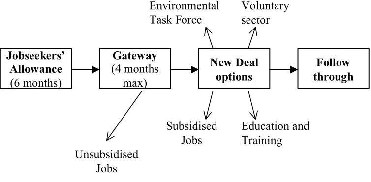
The path of a participant through the New Deal is composed of three main steps (see Figure 1). On assignment to the program, the individual starts the first stage of the treatment called the “Gateway”. This is the part of the program being evaluated in the present study. It lasts for up to four months and is composed of intensive job-search assistance and small basic skills' courses. Each individual is assigned a “Personal advisor”, a mentor who they meet at least once every two weeks to encourage/enforce job search.

The second stage is composed of four possible options. First, there is the “employer option” - a six-month spell on subsidized employment. For the subsidized employment option, the employer receives a £60 (about $90) a week wage subsidy during the first six months of employment plus an additional £750 (about $1125) contribution to finance a required minimum amount of job training equivalent to one day a week10. Under a second possible option, individuals can enroll in a stipulated full-time education or training course and receive an equivalent amount to the JSA payment for up to twelve months. Third, individuals can work in the voluntary sector for up to six months and are paid a wage or allowance of at least the JSA plus £400 ($600) spread over the six months. Finally, they may take a job on the “Environmental Task Force” - essentially a government job11.

Once the option period is over, if the individual has not managed to keep/find a job or leave the claimant count for any other reason, the third stage of the program is initiated, the “Follow Through”. This is a process similar to the Gateway, taking up to thirteen weeks, where job-search assistance is the main treatment being provided.

The program was launched in the whole UK in April 1998 (the “National Roll Out”). There was, however, a pilot from January to March 1998, when the program was implemented in twelve areas, called the Pathfinder pilots12_{. Clearly, identification of the treatment effect under these conditions}

counterfactual must either be drawn from a different labor market or from a group with different characteristics operating in the same labor market. Below we explore what we can identify under different assumptions.

Given that the program has not been running for a long period, we focus in this paper on an evaluation of the Gateway. In particular, we are concerned with the degree to which enhanced job search assistance has lead to an increase in outflows to jobs. The evaluation is based on data provided by the Pathfinder areas before the National Roll Out of the program, as well as on data available following the National Roll Out.

In evaluating the impact of the program we need to consider the precise nature of the comparison group, and hence the definition of what is being measured, and the set of assumptions that underlie the interpretation of the parameter we estimate in each case. There are some important aspects covered within this discussion. One of them concerns the extent to which we can estimate the overall impact of the program on employment as opposed to the impact on the eligible individuals. Potential differences between the overall impact and the effect of treatment on the eligible group could arise because: (1) the impact of the program on eligible individuals may be at the expense of worsened labor market opportunities for similar but ineligible individuals or (2) the wider implementation of the program and the opportunities it offers to participants may affect the equilibrium level of wages and employment, affecting all workers.

II.2. Choice of the outcome variables

placements, then individuals close to the Gateway and eligible for the program may reduce their search effort and wait for the program. In this case, the average individual among eligibles would be more prone to leave unemployment than its counterpart in the comparison group, leading to increased exit rates for this group. However, we can test this hypothesis by estimating the proportion of those who left unemployment by the end of the sixth month in the eligible and ineligible group. Such a comparison will provide an idea of how important such compositional effects are likely to be.

We will pay special attention to the outflows into employment, but we also examine total outflows from unemployment to all destinations. To assess the importance of the estimated effects, we interpret them in an historical perspective. We provide some lower and upper bounds for the treatment effect by using our methodology during other pre-program time periods. This can be done for total outflow for all years since 1982.

To summarize: treatment is understood as the job-search assistance initiative of the New Deal and the treated are those who enroll in the program after completing a six month unemployment spell. We aim at measuring the impact of improved job-search assistance on the probability of finding a job among the treated. To assess the robustness of our results, we also present estimates of other parameters that are informative about the adequacy of the underlying assumptions. Different definitions of treatment and the treated often characterise such parameters, and this is made clear on the following discussion.

III. Identification and Estimation Methods

ones. The extent to which this may happen will depend on a number of factors. If the subsidy just covers the deficit in productivity as well as the costs of training, we would not expect any substitution; these workers are no cheaper than anyone else. Second, it will depend on the extent that these workers are substitutable in production for existing workers and on the extent that it is easy to “churn” workers, that is to replace a worker finishing a six-month subsidy with a new subsidized worker. The latter is an important point, since the subsidy only lasts six months. Moreover the agencies implementing the New Deal are supposed to be monitoring the behavior of firms using wage subsidies and employing individuals on the New Deal. Of course if job durations are generally short, firms will be able to use subsidized workers instead of the non-subsidized ones, without any extra effort.

The New Deal may also change the prices in a region or country as a whole as it affects a substantial number of people. For example, the increased search activities of the unemployed could lower the equilibrium wage for less skilled individuals and therefore increase aggregate employment through a higher job offer arrival rate. This will tend to increase employment for eligible and ineligible individuals and will counteract the effects of substitution on the non-treatment group. Randomized trials cannot account for these general equilibrium or “community wide” effects which have become an important issue in the program evaluation literature14.

Assessing the importance of substitution and of General Equilibrium effects through wages or other channels is of central importance. Using the comparison between the pilot and control areas as described below, and assuming these areas are sufficiently separate labor markets from each other, we will be able to assess the extent to which substitution and other General Equilibrium effects combined are likely to be important “side-effects” of the program, at least in the short run. Below we discuss the evaluation methodology, a central part of which is the choice of comparison group. This choice is to a large extent governed by the issues discussed above.

III.1 The Choice of Comparison Group

Define by 1 it

Y the outcome for individual i in period t they are exposed to the policy (treatment).

The outcome for the same individual if not exposed to the policy is 0 it

the i-th individual of the policy is 1 0 it it Y

Y − . The average policy impact for those going through the

New Deal is_E

(

)

it . This parameter will be the focus of our attention. ND=1 denotes

the areas assigned to the New Deal, t=0 represents the period before implementation and t=1 the period after. Quite clearly, the evaluation problem relates to the missing data that would allow us to

estimate _E

(

)

it directly. In this section we define a number of alternative comparison

groups that will allow us to estimate this counterfactual mean. As we will point out, the definition and interpretation of the estimated parameter will change in certain cases with the comparison group.

Consider first a contrast obtained by comparing employment growth in pilot areas to employment growth in control areas. Assume that

(1)

(

) (

)

(

) (

)

0 , 1 | 1 , 1 | 0 0 0 0 = = − = = = = = − = = t ND Y E t ND Y E t ND Y E t ND Y E it it it it

This assumption means that the growth in employment in the New Deal areas would have been the same as in the non New Deal areas in the absence of the policy. In this case the missing counterfactual value can be replaced by

(

) (

)

E 0 | =1, =1) = 0| =1, =0 +

This expression is simply the employment level in the New Deal areas before the policy was implemented, adjusted for aggregate employment growth, given by

(

) (

)

[

]

= EY ND t EY ND t

m_{t it it} .

We can, however, obtain a measure of the importance of substitution effects by comparing the growth of employment in pilot and control areas separately for eligible and ineligible individuals. Consider applying assumption (1) applied separately to eligible and ineligible individuals and computing the growth in the employment for the eligible individuals in the pilot and control areas separately. Substitution effects should increase the employment of eligible individuals at the expense of ineligible ones in the pilot areas. Area-specific general equilibrium effects due to the change in wage pressure from the increased supply of workers should tend to increase the employment of both eligible and ineligible individuals. The GE effects can be though of as part of the program effect. The employment growth of eligible individuals will include the “pure” program effect, the GE effect and the presumably positive substitution effect. The employment growth of ineligible individuals will include a GE effect and a substitution effect of equal and opposite sign to that of the treatment group (assuming that the comparison group is the only group of workers displaced due to the wage subsidy). Thus a sum of the estimated “treatment” effects on eligible and ineligibles in the pilot areas compared to the control areas (weighted by the size of each group) should provide us with an estimate of the program effect and the GE effect combined, but net of the substitution. If this is similar to an appropriately scaled version of the effect on eligibles alone we can infer that substitution effects are not an important issue.

groups, we are ruling out any substitution effects or equilibrium wage effects that impact on the groups in a differential way. In this case a comparison in the growth rates between eligible and ineligible individuals will provide an estimate of the impact of the program on the eligible ones.

The virtue of the comparison group - that it is very similar to the treatment group in terms of its characteristics and will therefore be expected to respond to shocks in similar ways - may be, in fact, its greatest disadvantage. The substitution effects are likely to be much more severe the closer are the productivity characteristics of two groups. In the event of substitution, the impact of the program for the eligible group is biased upwards by the fact that the employment of the comparison group is decreasing. If such a decrease is, say, β, the “true” net increase in employment is 2β lower than the estimated increase in employment. However the benefit in terms of employment for the target group would be β lower than our estimate. Within this framework of analysis, the only way we have of gauging the size of βis through the pilots, as discussed above. Alternatively a general equilibrium model would allow us to estimateβ, at least in the long run, based on the substitutability of the two groups in production.

The next important issue is whether the impact of the policy is heterogeneous with respect to observable characteristics. If this is the case, we should interpret the estimate we obtain as an average impact across different effects but must make sure that a suitable comparison group exists. One way to address this problem is to use propensity score matching adapted for the case of difference-in-differences. In this case, there are two assignments that are non-random. One assignment is to the eligible population and the other assignment is to the relevant time period (before or after the reform). For the evaluation to make sense with heterogeneous treatment effects, we must guarantee that the distribution of the relevant observable characteristics is the same in the four cells defined by eligibility and time. One way of achieving this is to extend propensity score matching by defining two propensity scores – one for eligibility and one for time period. We then create a matched sample based on the two propensity scores. This approach ensures that the distribution of observed characteristics is balanced across all cells. In general, the assumption required to justify this approach is that

(

) (

)

(

) (

)

1 , 1 , | 0 , 1 , | 0 0 0 0 = = − = = = = = − = = t ND X Y E t ND X Y E t ND X Y E t ND X Y E it it it it

where ND=1 denotes eligibility and t the time period. This allows the time effects to differ by X. Following Dearden et al. [2001], under this assumption it is possible to construct matched samples by conditioning on the propensity scores for eligibility,P_EX =Pr

(

)

(

)

(2)

(

) (

)

(

) (

)

1 , 1 , , | 0 , 1 , , | 0 0 0 0 = = − = = = = = − = = t ND P P Y E t ND P P Y E t ND P P Y E t ND P P Y E tX EX it tX EX it tX EX it tX EX it

Finally the discrete nature of our outcome variable may imply that the assumptions we make do not hold for the expectations (which are employment probabilities) but for some transformation thereof; in particular for the inverse of the probability function, which must be assumed known. In this case we assume that

(

)

[

]

[

(

)

]

(

)

[

]

[

(

)

]

0 , 1 , | 1 , 1 , | 0 1 0 1 0 1 0 1 = = − = = = = = − = = − − − − t ND X Y E f t ND X Y E f t ND X Y E f t ND X Y E f it it it it

where _f−1 _{is the inverse of the probability function (e.g. the inverse logistic). This just says that the}

assumption we make is valid for the index rather than the probability itself. Define by Yit the

employment indicator for individual i in period t. In the New Deal areas in period t=1, this will represent the outcome under treatment. In all other cases it will represent an outcome under non-treatment. The impact of the policy can then be evaluated as

(3) I

( )

(

)

[

(

(

) ( )

α

)

]

where

(4)

{

[

(

)

]

[

(

)

]

}

(

)

[

]

[

(

)

]

{

}

0 , 1 , | 1 , 1 , | ) ( 1 1 1 1 = = − = = − = = − = = = − − − − t ND X Y E f t ND X Y E f t ND X Y E f t ND X Y E f X it it it it α

III.2 Implementation

Given a particular choice of comparison group, all methods we apply have the same structure as implied by (3) and (4). They differ only in the way that the expectations in these expressions are computed.

In the linear matching Difference-in-Differences estimator we run the following simple regression on the sample of comparison and treatment observations

it it it

t ND

it d X ND

Y =θ + +γ' +α +ε

where Y_it is a discrete variable indicating whether the person is in employment or not, θ_ND is an

eligibility specific intercept (may it be area or age defined or both, depending on the comparison

group used), d_t reflects common/aggregate effects and whereXis included to correct for differences

in observable characteristics between individuals and areas registered at the eligibility point (completion of the 6th month in unemployment).

These procedures can be quite restrictive in a number of ways. First, they do not allow for α to depend on X. And second, they do not impose common support on the distribution of the Xs across all four cells. The first assumption can be relaxed under the parametric setting, and this is what we do within the non-linear logit specification. The effect of treatment is allowed to depend on the observable characteristics of the agents by applying the following estimation technique. A different relationship between the outcome and the observables is estimated by group of agents - eligibility status (area or age) interacted with time. Such relationships entail the particular behaviour pattern of each group and the impact of treatment when it existed. By predicting the outcome of treated under the non-treated behavioural equation one obtains an estimate of how the treated would have been without the treatment would they belong to each of the other groups conditional on their observable characteristics. Applying difference-in-differences to such predictions using equation (3) produces an estimate of the expected impact of treatment on the treated.

distribution of the X characteristics in the treatment and comparison samples, before and after the reform. The matching method we use smoothes the counterfactual outcomes either with a Kernel based method or with splines (see, Heckman, Ichimura and Todd, 97 and Meghir and Palme, 01). We also present results based on the nearest neighbour weighting scheme. These however turn out to be much less precise. We provide details on the estimation method in Appendix 3.16

III.3. Other estimation issues

III.3.1. The choice of comparison areas

As discussed above, the available options for the choice of the comparison group depend on the type of evaluation being performed. When assessing the program from data on its National Roll Out, we are constrained to use ineligible individuals within the same area, for which we have chosen the age rule to define (in)eligibility. For the pilot study, however, the regional rule provides an additional instrument in the definition of the comparison group. We have used it in two ways, constructing two possible comparison groups: The first takes all eligible individuals living in all non-Pathfinder areas; the second selects all eligible individuals in the set of non-Pathfinder areas that most closely resemble the Pathfinder areas in a way detailed below.

period for comparison and in the results section we are careful to test the sensitivity of the results to alternative timing assumptions.

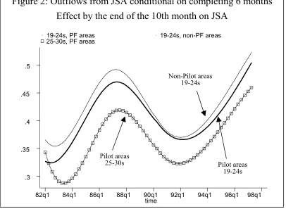
When using all eligible individuals in non-Pathfinder areas as a comparison group (or a matched sub-sample of them), it is being assumed that the two curves represented in Figure 2 are indeed parallel so that similar individuals are similarly affected by macro trends, independently of where they live. One can, however, choose the areas that more closely follow the cycle pattern identified for the Pathfinder areas. This can be done either within each of the matching procedures described above, or prior to them, selecting the areas where the comparisons are to be drawn from. We have chosen to adopt this latter option, matching the areas in a first step and applying all types of estimators comparing eligibles in different areas to the sub-samples obtained. In this procedure, we have used a completely non-parametric technique, as described below.

The aim of matching the areas is to achieve a match as close as possible with respect to labor market characteristics. The procedure followed to match on labor market characteristics makes use of a quarterly time-series of the outcome variable from 1982 to just before the introduction of the New Deal, in January 1998. A measure of distance was then computed for each possible pair of Pathfinder and non-Pathfinder areas and the two nearest neighbors were chosen. Once the two nearest neighboring areas have been chosen based on similarity of the labor market trends, we carry out the estimation procedure as described earlier.

III.3.2. Sensitivity of the results

The relative size of the estimated impact of the program, when viewed in an historical perspective, can inform on how significant the result is. In order to do so, the series of year-by-year estimates of the impact of a fictitious program has been computed.18 _{Given the lack of data on}

“destination when leaving JSA” before August of 1996, we use information on “exits to all destinations” to perform this analysis.

differential aggregate variation that is not being controlled for and is captured by the program dummy. In such a case, doubts are raised on whether the estimated effect is actually capturing the causal effect of the program alone. We can go further and bound the estimated impact of the Gateway using the distribution of year-by-year estimates to construct an upper and lower bound to the estimated effect. This is done by taking the percentiles on the tail of the distribution - say, percentiles five and ninety-five or ten and ninety - as being the expected value of the estimates in the absence of a program, and using them to re-scale the estimated impact up or down accordingly.

III.3.3. Compositional changes in the treatment group

Such a large-scale program may have compositional effects on the group of eligible individuals. Having learned about the eligibility rules, potential participants may change their behavior in order to secure or avoid enrolment. If such a selection process is taking place, the estimated effects of the program will be affected because the groups being compared are not what they would have been in the absence of the program. We check for this selection bias by examining difference-in-difference estimates of individuals’ probabilities of exiting unemployment in the pre-treatment period (i.e. in the months before reaching six months unemployment when the program begins).

IV. Data

are twenty different destination codes, including exit to employment, training/education, other benefits, incarceration, etc. The JUVOS data set also includes a small number of other variables - age, gender, marital status, geographic location, previous occupation and sought occupation. Descriptive statistics on the treatment group and different comparison groups are presented in Appendix1, Table 1A.

We also make use of the New Deal Evaluation Dataset (NDED), an administrative data set that contains information on virtually all individuals that have gone through the New Deal, even if only briefly. For participants, very detailed information is available from the time they join the program, including the types of treatment being administered and the timing of each intervention, letters being sent and interviews being made, a long list of socio-demographic variables and the destination when leaving the program. Non-participants, however, are not included in the sample, which limits its use for evaluation purposes. Note that we only consider the flow at six months, so there is no direct problem with mixing the stock and flow.

The use of the evaluation dataset NDED is meant to complement the lack of information in benefit (JSA) administrative records about the take-up of New Deal options. Since starting an option implies dropping from the JSA claimant count, there is a potentially large group that is being re-classified as non-unemployed while simply being driven through the program according to its rules. Unfortunately, we are unable to securely identify these types of exits from the JUVOS data set.19 We use the NDED instead to know the proportion of participants that enroll in each type of option (in any given region-date) by length of the New Deal spell.

In drawing up the treatment groups we have used 19-24 year olds even though the New Deal also affects 18 year olds. This is because 18 year olds can still be in high school and in England high school is only compulsory up to the age of sixteen. Participation of 16 to 18 year olds in full time education grew rapidly over this period so we decided to avoid any time varying composition effects by dropping 18 year olds. In any case, inclusion made no difference to the results.20

date is April 1999). We match this with the individuals who finished a 6-month JSA spell between April and December 1997. For the Pilot Study we compare individuals completing a 6-month JSA spell between the start of January and the end of March 1998 in the Pathfinder areas to the same group in January through March 1997. Ending the sample in April 1999 has the advantage that we avoid contaminating the New Deal effect with the introduction of the national minimum wage enforced from April 1999 onwards.21

Some information on the macro-economic climate is given in Figure 3. The New Deal was introduced at a favorable point of the business cycle by historical standards. There was no rapid improvement in the labor market between Spring 1998 and 1999, however, unlike the previous 12 months. The changing business cycle illustrates the reason why we have to select our comparison groups carefully in implementing our approach to ensure that these macro trends are “differenced out”.

Finally, it should also be pointed out that the effects of the program in this favorable climate may not be easily applied to less favorable periods. First the pool of unemployed is likely to be of worse quality when the aggregate economy is booming. Opposing this is the fact that, in the presence of firing costs (formal or informal) hiring someone in boom may be less risky.

V. Results

V.1. Pilot Study: men’s results

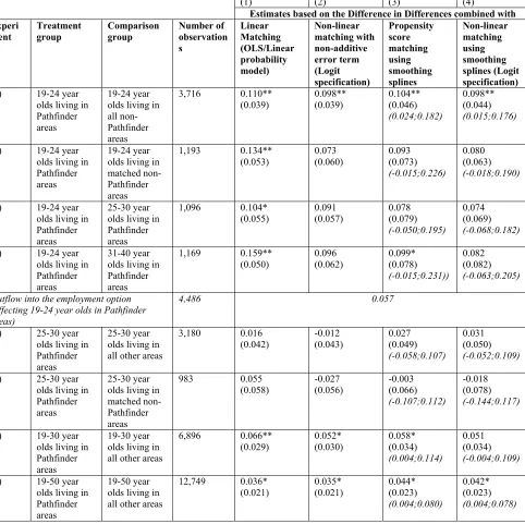
Table 1 presents the main estimates of the impact of the Gateway on eligible men living in Pathfinder areas during the pilot period. We consider a number of different possible comparison groups, providing some insight on the possible size of indirect effects. Each row in the table corresponds to a different comparison, including different estimates, obtained under different methods, of the effects of the Gateway on outflows to employment after four months of treatment.22

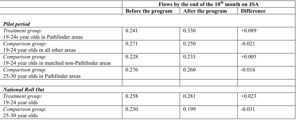
The first row of Table 1 compares men aged 19 to 24 years old living in Pathfinder areas to other 19 to 24 year-old men (with the same unemployment duration) living in all non-Pathfinder areas. After four months of treatment, it is estimated that the Gateway has improved participants' exits into employment very significantly – all the estimators point to an impact of about ten to eleven percentage points. This effect is even more impressive if compared with the outflow rates reported in Table 2. In the pre-program period only twenty-four per cent of individuals in the treatment group obtained employment over the similar four months period (compared to thirty three per cent afterwards). Thus, the improved job-search assistance provided during the Gateway seems to have raised the probability of getting a job by about 42 per cent (= 10%/24%) after four months of treatment.

.

percentage points. Thus, four percentage points is a lower bound for the pure Gateway/job assistance effect. The method used to estimate the impact of treatment does not seem to substantially influence the results, reflecting some robustness of the estimates to the functional form assumptions.23

The rest of the rows in table 1 present estimates for some of the other identifiable parameters discussed in section 3, also providing some clues about the robustness of the results. We start by restricting the comparison group to be composed of eligible men living in matched non-Pathfinder areas in the second row. Depending on the method used, the estimated effect may rise or fall slightly, but not significantly so. This evidence supports the comparability of the two groups used in row 1.

effects or differential trends across regions we may find differences in outflows in the New Deal period. In fact, no significant effects of the New Deal on non-eligibles are found.

Finally, rows 7 and 8 in table 1 contain estimates of the employment effect in the “whole market”. Men aged 19 to 30 and 19 to 50 years old and living in Pathfinder areas are compared with similar individuals living in non-Pathfinder areas. The results only confirm what has been established before: that, during the pilot period, the program had a very significant positive impact on outflows to employment in the markets it has been implemented. The point estimates are smaller because 19-24 year olds are only a fraction of the larger age range. For example, just over half the 19-30 year old group are 19-24 year olds. The linear matching estimator in row 7 implies a New Deal effect of 6.6 percentage points – as expected just over half the magnitude of the effect in row 1.

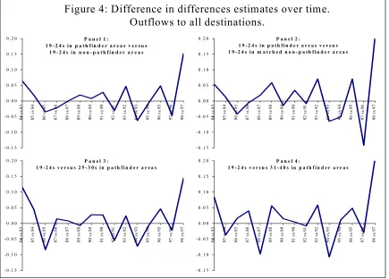
It is interesting to check how sensitive these results are to historical patterns. The lack of information about destinations when leaving the claimant count before 1996 imposes the use of a different variable, outflows to all destinations, to perform this analysis. Figure 4 considers different types of comparisons and plots the estimates of non-existent programs over time. The first panel in the chart compares eligible individuals living in Pathfinder areas with eligible individuals living in all other areas. The size of the New Deal effect, represented by the last point in the graph, is well above all other estimates for previous periods. This is just more evidence that the effects of the program on participants during the pilot period are very positive. Panel 2 compares participants with eligible individuals living in matched non-Pathfinder areas. It shows a similar pattern but with a stronger effect of the New Deal, which may be a consequence of the higher volatility observed. Panel 3 and 4 also confirm the importance of the estimated impact of the New Deal by comparing participants with older groups.

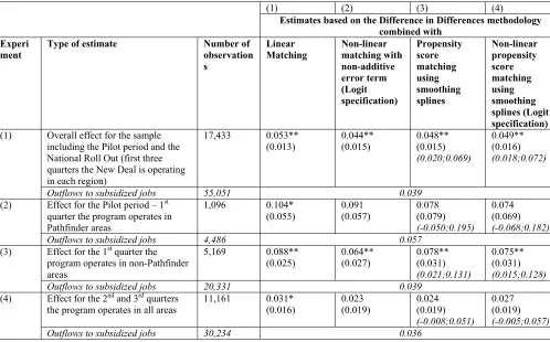
V.2. National Roll Out: men’s results

impact, it is about half the magnitude estimated for the pilot period. These differences in size can be accounted for by a “program introduction” effect. In the first few months the program is operating, a very large increase in the flows to employment is observed, which then falls as the program matures. This is illustrated in the other rows of the table. The second and third rows report comparable estimates of the Gateway effect after 4 months of treatment for the first quarter the program operates in the Pathfinder and non-Pathfinder areas, respectively. As noticed before, estimates for the pilot period (first quarter in Pathfinder areas) are about twice the size of the effect over the whole period. The same is also true if one considers the estimates for the first quarter the New Deal operates in non-Pathfinder areas (see row 3). The fourth row presents estimates obtained using the following second and third quarters the program is operating and these are comparatively much lower and less significant.

There are, of course, many possible explanations for this. One explanation is that the agencies involved in delivering the program are initially very enthusiastic, but this naturally erodes over time. Another possibility is that the program diminishes welfare fraud. This would have particularly important effects during the first few months after the release of the program since potential participants are unlikely to be aware of the new claiming rules. Similar “cleaning up the register” effects have been noted of previous UK labor market reforms.24

There are many possible criticisms of the results. We shall now discuss some of the main ones - quality of job matches, selectivity and differential trends. How the program affects the women will be discussed on the next section.

outflow to sustained jobs (instead of any job) as the outcome variable. The results are quite consistent with the earlier findings – the estimates point to an increase in the outflows to sustained jobs of 4.5% (in column 1 of Table 4), which compares to estimates of around 5% for the outflows to all employment (in column 1, first row of Table 3).

Secondly, there is the issue of selectivity. It may be that the introduction of the New Deal has an effect on the (unobserved) quality of the inflow of individuals reaching six months of JSA. The most likely route for this is that claimants in the fifth or sixth months of JSA may alter their behavior. If they believe the New Deal regime is “tougher” than the previous regime, they may be more likely to leave the unemployment rolls (this was one of the ways that RESTART, another job assistance program introduced in 1986 was deemed to have worked). On the other hand, if the New Deal is seen as a desirable thing (e.g. because of subsidies to “good jobs” or training), then claimants may delay exit. If the main effect is increased toughness, then we may underestimate the positive effects of the New Deal as there has been a decline in the unobserved quality of the stock (assuming the most job ready decide to leap into jobs before they are pushed off the unemployment rolls). If the New Deal is perceived as more attractive than the previous regime (as the qualitative evidence suggests) then we may actually be overestimating the effects of the Gateway period as the more job ready actually delay their exits prior to entering the Gateway.

To investigate these selectivity problems we examine outflows to employment during the fourth and fifth month of JSA, using the same methodology as before. The results are presented in rows 2 and 3 of Table 4, Panel B. The introduction of the New Deal had no significant impact on the outflows to employment prior to six months duration. All the estimates are small and insignificant at conventional levels.

V.3. The impact of the program on women

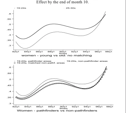
Finally, note that we have focused our results on male job outflow rates. Three quarters of all participants in the New Deal are men, but clearly the impact on women is also of great interest. The results for women are not as clear-cut as those for men. This is mainly because there is a systematic trend in the labor market behavior of older (25-30) compared to younger (19-24) women. The main problem, therefore, resides on the choice of the appropriate comparison group.

Figure 5 illustrates the difficulties encountered by plotting the conditional exits to all destinations against time for treatments and different possible comparison groups. It is apparent from the upper panel of Figure 5 that an estimator based on different age groups can be severely contaminated by differential trends. Compared to the younger age groups, the older age groups seem to have systematically improved their position in the labor market over the 1982-99 period. If this trend extends to the treatment period, it is expected that such comparison under-estimates the impact of treatment on the treated. On the other hand, the lower panel of the graph suggests that the macro shocks seem to affect younger age groups living in different geographic regions much more similarly, making the Pathfinder – non Pathfinder 19-24 year old groups comparable. Matching on regions improves the pattern, the two curves for treatment and comparisons being closer both in levels and slopes. The upshot of this is that using older women as a comparison group is not valid, and we should focus on the Pathfinder data to evaluate the effect of the New Deal for women.

remaining statistically insignificant, the estimates are actually negative. Together with the pattern depicted in figure 5, this explains why the women’s case is not explored during the National Roll Out of the program. The only group we can draw comparisons from is composed of individuals older than the participants, and these are subject to very differential trends.

V.4 Discussion of the results: A comparison with the existing literature

How do our findings compare with the existing results? We overlap with several other program evaluation literatures: Unemployment Insurance (UI) reform, wage subsidies, youth measures over education and training. Perhaps the most directly relevant are the recent program evaluations of mandatory job search associated with welfare to work reforms. Bloom and Michalopoulos [2001] survey 29 different initiatives that had demonstration projects. Eight of these schemes were job-focused (rather than education/training job-focused) and mandatory for welfare recipients. Table 6 summarizes the results from these studies and shows that although the precise impact effect differed probabilities was found in all eight cases. The median of the impacts in the final column of Table 6 is 0.23, which is not wildly out of line with our “central” estimate of a program impact of 0.2. Again we should note that 0.2 is probably an ‘upper bound’ measure since, as we have noted, a large part of this employment effect is towards subsidized jobs and also due to a “first quarter” effect.

effective. It is interesting to note that in the study of worker profiling and reemployment services which involves mandatory employment and training services, Black et al (2003) find most of the impact to be a sharp increase in early exits from UI coinciding associated with claimants finding out about their mandatory program obligations.

A feature of the New Deal is that it is youth-focused. Most evaluations of youth initiatives have been pessimistic, especially for young men (for example, Heckman, LaLonde and Smith [1999]). Our study gives some room for optimism, but it should be remembered that the participant group for most U.S. youth training programs are quite different from the British New Dealers. U.S. schemes are focused on very disadvantaged youth – for example, long-term unemployment is rare in the US, but more common in Europe. It may be easier to help the young in the New Deal because they are far more “job-ready” than their U.S. counterparts. In addition (unlike JTPA) we are not looking at the impact of the training/education aspects of the New Deal and have focused only on the mandatory job search and wage subsidy element.

Finally, there is an extensive literature on the role of financial incentives for employers and individuals in encouraging employment amongst the less skilled. Employer-based job subsidies of the kind discussed here are rarer than individual-based incentives such as EITC.25 Both types of policy can be successful in raising employment26_{, but this conclusion depends very much on the}

exact program. A major problem with employer-based wage subsidies is that they have very low take-up by employers, perhaps due to stigma or administrative burden.27

VI. Conclusions

This paper has examined the labor market impact of the British New Deal for Young People. The New Deal is a compulsory program affecting all young people claiming unemployment benefit for at least six months. The program offers a combination of treatments, particularly job assistance for four months and a wage subsidy paid to employers. Two sources of identification are used to construct comparison groups in order to make inferences on the impact of the New Deal: a comparison between pilot areas and non-pilot areas and age-related eligibility criteria. Our results suggest similar quantitative effects whichever comparison group is chosen.

Based on the pilot period of the program we find an economically and statistically significant effect of the program on outflows to employment among men. The program appears to have caused an increase in the probability of young men (who had been unemployed for six months) finding a job in the next four months. On average, this increase is about 5 percentage points (relative to a pre-program baseline of about 26 per cent). Part of this overall effect is the job subsidy element and part is a pure enhanced job search. We estimate that at least 1 percentage point of the 5 percentage points is due to the Gateway services, such as job search assistance (rather than the wage subsidy element). We also found that the treatment impact is much larger in the first quarter of introduction compared to the subsequent two quarters. This puts in question whether the effects of this aspect of the program will be sustained in the long run. Our findings are robust to a large number of experiments, including a number of different comparison groups.

There are at least three areas of further work. First, the main omission in our work is that we do not consider the longer-term effects of the New Deal. A full evaluation needs to consider whether individuals’ employability has been enhanced by their experience of subsidized work and education and training. The data is only just becoming available to perform such an analysis. A second problem lies in untangling how robust our estimates are in the face of substitution and equilibrium wage changes. To take these into account involves putting more economic structure on the problem than we have done in this paper (e.g. Blundell, Costa Dias and Meghir, 2003). It is reassuring, however, that the Pathfinder pilots vs. non-pilot comparisons yielded results that were quantitatively similar to the within Pathfinder analysis. Finally, we have eschewed a formal cost-benefit analysis given the uncertainty surrounding some of the benefits such as the training and education option. However, this is clearly an important next step that will be informed by some of the estimates obtained in this paper.

Appendix 1: Data

Table 1A compares the mean values of some of the independent variables used in the analysis before and after matching on the propensity scores.28 It can be observed that similar age groups are much more alike, at least with respect to the considered characteristics (compare columns 1 and 2 with 5 and 6). Moreover, matching on the propensity scores significantly improves the similarity between the groups (compare columns 3-4 with 1-2 or columns 7-8 with 5-6).

precisely. Moreover, nearly all the initial support is maintained after matching. Figures 2A to 4A give some indications of how identical the distributions of the propensity scores are over sub-groups of the population. It is apparent that matching worked well even over sub-populations, making the distributions quite similar. Very similar results were obtained when using other groups and are available under request.

Appendix 2: Gateway employment effects under different propensity score

matching techniques

Appendix 3: Estimation methods

The practical implementation of the completely parametric methods is discussed in the main text, and so we omit it here. We use propensity score matching based on two dimensions, time and eligibility, and using either the nearest neighbor method or smoothing the outcomes applying splines or kernel weights. With the same set of observables used in the completely parametric estimates, we compute the two propensity scores, P_1X =P

(

)

(

)

In the nearest neighbor case, each treated individual is paired with one observation from each of the three comparison groups, the one that minimizes the Euclidean distance with respect to the two propensity scores conditional on two maximum distance restrictions, one for each dimension. Matching is done with replacement, meaning that each comparison observation may be chosen more than once and is weighted accordingly.

Under the smoothing splines method, we run a regression of the outcome of interest on a cubic polynomial of the two propensity scores for each of the comparison groups. Predictions of the outcome under the three non-treatment cases for each of the matched treated observations under the nearest neighbor method are then computed and used to estimate the impact of treatment.

The use of kernel weights to select each of the three comparison groups is based on the Epanechnikov function and a diagonal matrix of (constant) bandwidths, each element of the diagonal

being given by _{1.06 n}−1/5 x

σ .

Appendix 4: UK Unemployment Benefit Rules

The main benefit available for unemployed young people is Jobseeker's Allowance (JSA). It was introduced in October 1996 to replace unemployment benefit. The level of JSA was about £40 a week throughout the New Deal period, though this amount depends on the age of the applicant, and the respective household income and needs. To be eligible for JSA, an unemployed person must: (i) Be “actively seeking work”, which is assessed by a fortnightly short interview taking 5-10 minutes; and (ii) Meet some conditions concerning the past two tax years working history, related to the amount of National Insurance contributions made while employed (“contributory JSA”) or, alternatively, pass a “means test”. Thus, it is possible for someone who never worked before to be entitled for the benefit. In a reform in 1986 (RESTART) more intensive job focused interviews took place at six monthly interviews.

If not before, receipt for JSA becomes “means tested” after six months. Individuals with income from other sources (large assets or a partner bringing in income) have their JSA scaled down or taken away altogether. Prior to October 1996, this period of “non-means tested” unemployment benefit was one year. The JSA imposes no time limit: as long as the conditions are met, an applicant is entitled to it.

References

Anderson, B., R. Riley and G. Young (1999), The New Deal for Young People: Early Findings from the Pathfinder areas. Employment Service Research and Development Employment Service Research, No. 34,

Anderson, P. “Monitoring and Assisting Active Job Search” Dartmouth College mimeo

Abbring, J., van den Berg, G., van Ours, J. (1997) “The effect of unemployment insurance sanctions on the transition rate from unemployment to employment” Tinbergen Institute Working Paper

Ashenfelter, O. and Card, D. (1985), ''Using the Longitudinal Structure of Earnings to Estimate the Effect of Training Programs'', Review of Economics and Statistics, 67, 648-660.

Ashenfelter, O., Ashmore, D. and Dechenes, O. (1999) “Do Unemployment Insurance Recipients Actively Seek Work? Randomized trials in four U.S. states” National Bureau of Economic Research Working Paper No. 6982

Bassi, L. (1983), “The Effect of CETA on the Post-Program Earnings of Participants”, Journal of Human Resources, Fall, 539-556.

Bassi, L.(1984), “Estimating the Effects of Training Programs with Nonrandom Selection”, Review of Economics and Statistics, 66, 36-43.

Bell, B., Blundell, R. and Van Reenen, J. (1999), “Getting the Unemployed Back to Work: An Evaluation of the New Deal Proposals'', International Tax and Public Finance, 6, 339-360.

Black, D, J. Smith, M. Berger and B.Noel (2003) “Is the Threat of Reemployment Services More Effective than the Services Themselves? Evidence from Random Assignment in the UI System.”

American Economic Review, forthcoming.

Blank, R., Card, D. and Robbins, P. (2000) “Financial Incentives for Increasing work and income among low income families” in Card, D. and Blank, R. (eds) Finding Jobs, New York: Russell Sage Foundation

Bloom, D. and Michalopoulos, C. (2001) “How welfare and work policies affect employment and income: A Synthesis of Research”, MDRC, May

Blundell, R. and M. Costa Dias (2000), “Evaluation Methods for Non-Experimental Data”, Fiscal Studies, March.

Blundell, R., M. Costa Dias and Costas Meghir (2003), “The overall impact of wage subsidies under idiosyncratic uncertainty”, mimeo, Institute for Fiscal Studies.

Blundell, R., Dearden, L., Goodman, A. And Reed, H. (1997), Higher Education, Employment and Earnings in Britain, Institute for Fiscal Studies Monograph Series.

Blundell, R., Duncan, A. and Meghir, C. (1998), “Estimating Labor Supply Responses using Tax Policy Reforms”, Econometrica, 66, 827-861.

Burtless, G. (1995), “The Case for Randomised Field Trials in Economic and Policy Research”,

Journal of Economic Perspectives, 9, 63-84.

Burtless, G. (1985) “Are targeted wage subsidies harmful? Evidence from a wage voucher experiment” Industrial and Labor Relations Review, 39, 105-114

Card, D. and Hyslop, D. (2002) “Estimating the dynamic effects of an earnings subsidy for welfare leavers”, mimeo, University of California, Berkeley

Davidson, C. and Woodbury, S. (1993) “The displacement effects of reemployment bonus programs”

Journal of Labor Economics, 11, 4, 575-605

Dearden, L, C. Emmerson, C. Frayne, A. Goodman, H. Ichimura, C. Meghir (2001) Evaluating the Education Maintenance Allowance in the UK, mimeo Institute for Fiscal Studies, invited presentation Royal Economic Society conference 2001.

Deheijia, R. and Wahba, S. (1998) “Propensity Score Matching Methods for non-experimental causal studies” National Bureau of Economic Research Working Paper No. 6829

Dehejia, R. and Wahba, S. (1999) “Causal Effects in Non-experimental studies: Reevaluating the evaluation of training programs” Journal of the American Statistical Association, 94, 448, 1053-1062

Dias, M. (2000), “Evaluating the Overall Effects of Active Labor Market Policies”, mimeo, Institute for Fiscal Studies.

Dolton, P., Makepeace, G. and Treble, J. (1992), “Public and Private Sector Training of Young People in Britain”, in L.M. Lynch (ed.), Training and the Public Sector, Chicago: University of Chicago Press.

Dubin, J. and Rivers, D. (1993) “Experimental estimates of the impact of wage subsidies” Journal of Econometrics, 56, 219-242

Eissa, N. and Leibman, J. (1996) “Labor Supply response to the Earned Income Tax Credit”

Quarterly Journal of Economics, 111 (May) 605-637

Fraker, T. and Maynard, R. (1987) “The adequacy of comparison group designs for evaluations of employment related programs” Journal of Human Resources, 22, 194-227

Hahn, J., Todd, P. and Van der Klaauw, W. (1999), “Identification and Estimation of Treatment Effects with regression Discontinuity Design”, Working paper, UNC, November.

Hales, J., Collins, D., Hasluck, C. and Woodland, S. (2000) “Mew Deals for the Young People and Long Term unemployed: Survey of Employers” Employment Service Report No. 58.

Hausman, J., and Wise, D. (1985), Social Experimentation, NBER, Chicago: University of Chicago Press.

Heckman, J. (1979), “Sample Selection Bias as a Specification Error”, Econometrica, 47, 153-61.

Heckman, J., Ichimura, H. And Todd, P. (1997), “Matching as an Econometric Evaluation Estimator: Evidence from Evaluating a Job Training Program”, Review of Economic Studies, 64, 605-654.

Heckman, J., R. LaLonde and J. Smith (1999) “The Economics and Econometrics of Active Labor Market Programs” in Handbook of Labor Economics, Volume 3 O. Ashenfelter and D. Card eds., 1865-2097

Heckman, J. And Robb, R. (1985), “Alternative methods for Evaluating the Impact of Interventions”, in Longitudinal Analysis of Labor market Data (New York: Wiley).

Heckman, J. And Robb, R. (1986), “Alternative methods for Solving the Problem of Selection Bias in Evaluating the Impact of Treatments on Outcomes”, in Howard Wainer (ed.), Drawing Inferences from Self-Selected Samples (Berlin: Springer Verlag).

Heckman, J. and Hotz, V. (1989) “Choosing among alternative nonexperimental estimators for estimating the impact of social programs” Journal of the American Statistical Association, 84, 862-874

Heckman, J., Smith, J. And N. Clements, (1997), “Making the Most out of Program Evaluations and Social Experiments: Accounting for Heterogeneity in program Impacts”, Review of Economic Studies, 64, 487-536.

Knab, J. Bos, J., Friedlander, D. and Weissman (2000) “Do mandates work? The effects to enter a Welfare to Work Program” Manpower Development Research Corporation, November.

Katz, L. (1998) “Wage Subsidies for the Disadvantaged.” in Generating Jobs, Richard Freeman and Peter Gottschalk, eds., New York, NY: Russell Sage Foundation, pp. 21-53.

Katz, L. and Meyer, B. (1990) “Unemployment Insurance, Recall Expectations and Unemployment Outcomes” Quarterly Journal of Economics, 105(4), 973-1002

Lalonde, R. (1986), “Evaluating the Econometric Evaluations of Training Programs with Experimental Data”, American Economic Review, 76, 604-620.

Layard, R. (2000) “Welfare to work and the New Deal” The Business Economist, 31, 3, 28-40.

Meyer, B. (1990) “Unemployment Insurance and Unemployment Spells” Econometrica, 58(4), 757-82

Smith, J. and P.Todd (2003), “Does Matching Overcome LaLonde’s Critique of Nonexperimental Estimators?” Journal of Econometrics, forthcoming.

Van Reenen, John (2001), “Active Labor Market Policies and the British New Deal for Unemployed Youth in Context" Institute for Fiscal Studies Working Paper No. 01/09 forthcoming in Richard Blundell, David Card and Richard Freeman (eds.) Seeking a Premier League Economy, University of Chicago Press.

Woodbury, S. and Spiegelman, R. (1987) “Bonuses to Workers and Employers to reduce unemployment: randomized trials in Illinois” American Economic Review, 513-30

Endnotes

1 _{LaLonde [1986] is perhaps the most influential paper expressing this view (see Heckman and Hotz, 1989, for}

an early riposte). Recently, Dehejia and Wahba [1998, 1999] have argued that careful matching using

propensity score methods can overcome many of the problems with conventional non-experimental estimators and sought to demonstrate this using LaLonde’s original data on the National Supported Work (NSW)

program. Smith and Todd [2000], however, showed that such “success” came from discarding a large

proportion of the original NSW data and that cross sectional matching estimators remained highly sensitive on the full sample. As with our own results presented here Smith and Todd found difference in differences estimators are the most robust.

2 _{This is the main British form of unemployment insurance (see Appendix 4).}

3 _{For more information about training programs in Britain and their effects see, for instance, Dolton,}

Makepeace and Treble [1992], Blundell, Dearden and Meghir [1996] and Blundell, Dearden, Goodman and Reed [1997].

4 _{See Heckman [1979], Heckman and Robb [1986], Blundell, Duncan and Meghir [1998], Bell, Blundell and}

Van Reenen [1999] and Blundell and Dias [2000] for precise descriptions of these conditions. Davidson and Woodbury [1993] is an example of an attempted calibration of substitution effects using data from the Illinois unemployment insurance (UI) experiments (see also Woodbury and Spiegelman, 1987, on this program).

5 _{See Card and Hyslop [2002] for evidence of the absence of dynamic effects in the Canadian Self Sufficiency}

Program.

6 _{For example, Knab, Bos, Friedlander and Weissman [2000] or Mofitt [1996].}

7 _{On job assistance see the survey by Meyer [1995]; on wage subsidies see Katz [1998].}

8 _{JSA is the main form of unemployment benefit in the UK. It is essentially a flat rate benefit paid every two}

week of about £40 ($60) a week. Past work experience is not a condition of receipt of JSA and although there is a requirement to “actively seek employment”. It is not time limited. See Appendix 4 for details.

9 _{Note that certain groups of especially disadvantaged individuals (e.g. the disabled, ex-convicts, those with}

obliged to enter the New Deal as they reached their 12th, 18th, 24th month, etc of JSA (unless they choose to be early entrants). We are careful to control for these “early entrants” in the work below.

10 _{This is quite generous. Hales et al [2000] find that the mean starting wage for those on a subsidized job is}

£3.78 an hour, implying a forty per cent level of subsidy for a thirty-seven hour week.

11 _{The intention was that the treatments were staged. The employment service would seek to place an}

individual in an unsubsidized job in the first month of the program, a subsidized job in the second month, in education/training in the third month and the Environmental Taskforce in the fourth month. This guidance was not strictly enforced on the ground, however.

12

See Anderson, Riley and Young [1999].

13 _{Our data currently ends in July 1999. Individuals entering the Gateway in April 1998 and joining the}

year-long education and training option after four months will only start job search in August 1999.

14 _{For example, Heckman, Lochner and Taber [1998].} 15 _{See Hahn, Todd and Van der Klaus [1999].}

16 _{The matching method we use smoothes the counterfactual outcomes either with a Kernel based method or}

with splines (see, Heckman, Ichimura and Todd, 97). We also present results based on the nearest neighbour weighting scheme. These however turn out to be much less precise.

17 _{We also considered more finely disaggregated age groups – e.g. 24 vs. 25 year olds – which generates}

similar qualitative results, although with much less precision on account of the smaller sample size.

18 _{This analysis is also informative on whether the assumptions on the comparability between any two groups}

being used are valid. In fact, before the introduction of the New Deal the estimated impacts are expected to be zero given the absence of a policy that causes a differential behavior between any two groups being compared. If, however, a large number of point estimates are found to be significantly different from zero, one might suspect that the assumptions on the comparability of the two groups being used are not valid.

19 _{There is a code in the JUVOS data which purports to have New Deal destinations, but on investigation it}

proved to be unreliable.

20 _{One could also worry about 18-22 year olds in college education. There is only a tiny fraction of this group}

in the unemployed pool, however.

21 _{Britain had never had a national minimum wage before this date. There was a system of Wages Councils}

that set minimum wages for certain groups of occupations in low wage industries. These only covered about two million of the approximately 30 million UK workforce when they were abolished in 1993 (see Dickens, Machin and Manning, 1999, for an analysis).

22 _{All regressions include a set of other covariates, including age (when similar age groups are being}

compared), marital status, region, sought occupation and labor market history variables. All computations have been performed excluding these covariates as well. Given the similarity of the results, however, we skip their presentation.

23 _{Appendix 1 presents some comparisons between treatment and comparison groups with respect with some}

of the covariates being considered, including a few checks on the quality of the propensity score matching.

24

See Van Reenen [2001] for discussion of Restart and the introduction of JSA.

25 _{See Eissa and Leibman [1996] for an evaluation.} 26

See Blank, Card and Robins [2001] for example.

27 _{Katz [1998]. See also Burtless [1985] and Dubin and Rivers [1993] for evaluations of wage subsidy}

programs.