Second order differential operators with interior singularity

(1)

R E S E A R C H

Open Access

Second-order differential operators with

interior singularity

Kadriye Aydemir

1*

_{and Oktay S Mukhtarov}

1,2

*_{Correspondence:}

[email protected]

1_{Department of Mathematics,}

Faculty of Arts and Science, Gaziosmanpa¸sa University, Tokat, 60250, Turkey

Full list of author information is available at the end of the article

Abstract

The purpose of this study is to investigate a new class of boundary value transmission problems (BVTPs) for a Sturm-Liouville equation on two separate intervals. We introduce a modiﬁed inner product in the direct sum spaceL2[a,c)⊕L2(c,b]⊕C2and

deﬁne a symmetric linear operator in it in such a way that the considered problem can be interpreted as an eigenvalue problem of this operator. Then, by suggesting own approaches, we construct the Green’s function for the BVTP under consideration and ﬁnd the resolvent function for the corresponding inhomogeneous problem.

Keywords: Sturm-Liouville problems; Green’s function; transmission conditions; resolvent operator

1 Introduction

Many interesting applications of Sturm-Liouville theory arise in quantum mechanics. For instance, for a single quantum-mechanical particle of massmmoving in one space dimen-sion in a potentialV(x), the time-dependent Schrödinger equation is

iψt= –



mψxx+V(x)ψ.

Looking for separable solutionsψ(x,t) =ϕ(x)e–iEt/, we find thatϕ(x) satisfies the differ-ential equation

–



mϕ

₊_V₍_x₎_ϕ₌_E_ϕ_.

That is a Sturm-Liouville equation of the form

–y+qy=λy.

The coeﬃcientqis proportional to the potentialV, and the eigenvalue parameterλis pro-portional to the energyE. Physical problems such as this and those involving sound, sur-face waves, heat conduction, electromagnetic waves, and gravitational waves, for example, can be solved using the mathematical theory of boundary value problems. Boundary value problems can be investigated also through the methods of Green’s function and eigenfunc-tion expansion. The main tool for solvability analysis of such problems is the concept of

(2)

Green’s function. The concept of Green’s function is very close to physical intuition (see []). If one knows the Green’s function of a problem, one can write down its solution in a closed form as linear combinations of integrals involving the Green’s function and the functions appearing in the inhomogeneities. Green’s functions can often be found in an explicit way, and in these cases it is very eﬃcient to solve the problem in this way. Deter-mination of Green’s functions is also possible using Sturm-Liouville theory. This leads to a series representation of Green’s functions (see []).

2 Statement of the problem

In this study we shall investigate a new class of BVPs which consist of the Sturm-Liouville equation

(y) := –p(x)y(x) +q(x)y(x) =λy(x) ()

to hold in a ﬁnite interval [a,b] except at one inner pointc∈(a,b), where discontinuities inyandyare prescribed by the transmission conditions at the interior pointx=c,

Vj(y) :=β_j–_y(c–) +β_j–_y(c–) +β_j+_y(c+) +β_j+_y(c+) = , j= , , () together with eigenparameter-dependent boundary conditions at end pointsx=a,b,

U(y) :=αy(a) –αy(a) –λ

α_ y(a) –α_ y(a)= , ()

U(y) :=αy(b) –αy(b) +λ

α_y(b) –α_ y(b)= , ()

wherep(x) =p–_{>  for}_x_∈_[_a_,_c_),_p₍_x_{) =}_p+_{>  for}_x_∈₍_c_,_b_{], the potential}_q₍_x_{) is a}

real-valued function continuous in each of the intervals [a,c) and (c,b], and it has a ﬁnite limit

q(c∓);λis a complex spectral parameter,αij,βij±,αij (i= ,  andj= , ) are real

(3)

(thermal conduction problems for a thin laminated plate) were studied in []. Boundary value problems with transmission conditions were investigated extensively in the recent years (see, for example, [, –, –]).

3 The ‘basic’ solutions and a characteristic function

With a view to constructing the characteristic function ω(λ), we shall deﬁne two basic solutionsϕ–(x,λ) andψ–(x,λ) on the left interval [a,c) and two basic solutionsϕ+(x,λ) and

respectively. In terms of these solutions, we shall deﬁne the other solutionsϕ+₍_x_,_λ_{) and}

ψ–(x,λ) by the initial conditions

(4)

It is convenient to deﬁne the characteristic functionω(λ) as

ω(λ) :=ω–(λ) =ω+(λ).

Obviously,ω(λ) is an entire function. By applying the technique of [], we can prove that there are inﬁnitely many eigenvaluesλn, n= , , . . . , of problem ()-() which coincide

with zeros of the characteristic functionω(λ).

4 Operator treatment in a modiﬁed Hilbert space

To analyze the spectrum of BVTP ()-(), we shall construct an adequate Hilbert space and deﬁne a symmetric linear operator in it in such a way that the considered problem can be interpreted as the eigenvalue problem of this operator. For this we assume that

> , > ,

θ=

α α

α_ α_

> , θ=

α α

α_ α_

> 

and introduce modiﬁed inner products on the direct sum spacesH=L[a,c)⊕L(c,b]

andH=H⊕Cby

[f,g]H:=



p–

c–

a

f(x)g(x)dx+

p+

b

c+

f(x)g(x)dx ()

and

[F,G]H:= [f,g]H+



θ

fg+



θ

fg ()

forF= (f(x),f,f),G= (g(x),g,g)∈H, respectively. Obviously, each of these inner

prod-ucts is equivalent to the standard inner prodprod-ucts of the Hilbert spacesL[a,c)⊕L(c,b]

andL[a,c)⊕L(c,b]⊕C, respectively, so (H, [·,·]H) and (H, [·,·]H) are also Hilbert spaces. Let us now deﬁne the boundary functionals

Ba[f] :=αf(a) –αf(a), Ba[f] :=αf(a) –αf(a),

Bb[f] :=αf(b) –αf(b), Bb[f] :=αf(b) –α f(b)

and construct the operatorL:H→Hwith the domain

dom(L) := F=f(x),f,f

:f(x),f(x)∈ACloc(a,c)∩ACloc(c,b),

and has a ﬁnite limitsf(c∓) andf(c∓),(f)∈L[a,b],

V(f) =V(f) = ,f=Ba[f],f= –Bb[f]

and action low

(5)

Then problem ()-() can be written in the operator equation form as follows:

LF=λF, F=f(x),B_a[f], –B_b[f]∈dom(L)

in the Hilbert spaceH.

Theorem  The linear operatorLis symmetric.

Proof By applying the method of [] it is not diﬃcult to show thatdom(L) is dense in the Hilbert spaceH. Now, letF= (f(x),B_a[f], –B_b[f]),G= (g(x),B_a[g], –B_b[g])∈dom(L). By partial integration we have

[LF,G]H– [F,LG]H=W(f,g;c–) –W(f,g;a)

+W(f,g;b) –W(f,g;c+)

+ θ

Ba[f]Ba[g] –Ba[f]Ba[g]

+ θ

B_b[f]Bb[g] –Bb[f]Bb[g]

, ()

where, as usual,W(f,g;x) denotes the Wronskians of the functions f andg. From the deﬁnitions of the boundary functionalsBaandBbwe get that

Ba[f]B_a[g] –B_a[f]Ba[g] =θW(f,g;a), ()

B_b[f]Bb[g] –Bb[f]B_b[g] = –θW(f,g;b). ()

Further, taking in view the deﬁnition ofLand applying the initial conditions ()-(), we derive that

W(f,g;c–) = 



W(f,g;c+). ()

Finally, substituting (), () and () in (), we have

[LF,G]_H= [F,LG]_H for everyF,G∈dom(L),

so the operatorLis symmetric inH. The proof is complete.

Corollary 

(i) All the eigenvalues of problem()-()are real.

(ii) Iff(x)andg(x)are eigenfunctions corresponding to distinct eigenvalues,then they are

‘orthogonal’in the sense of the equality

[f,g]H+



θ

B_a[f]B_a[g] + θ

B_b[f]B_b[g] = , ()

(6)

5 Solvability of the corresponding inhomogeneous problem Now, letλ∈Cnot be an eigenvalue ofL. Consider the operator equation

(λI–L)Y=U ()

for arbitraryU= (u(x),u,u)∈H. This operator equation is equivalent to the following

inhomogeneous BVTP:

(λ–)y(x) =u(x), x∈[a,c)∪(c,b], ()

V(y) =V(y) = , λBa[y] –Ba[y] =u, –λBb[y] –Bb[y] =u. ()

We shall search the resolvent function of this BVTP in the form

(7)

By diﬀerentiating we have

By using equalities (), () and boundary conditions (), we can derive that

h(λ) =

Let us introduce the Green’s function as

G(x,y;λ) =

Then from () and () it follows that the considered problem (), () has a unique solution given by

(8)

Theorem  The resolvent operator can be represented as

(λI–L)–U(x) =

⎛ ⎜ ⎝

b

a G(x,y;λ)u(y)dy+u

ψ(x,λ)

ω(λ) +u

ϕ(x,λ)

ω(λ)

B_a[u] –B_b[u]

⎞ ⎟ ⎠,

where

G(x,y;λ) =

_

p– G(x,y;λ) if a<y<c,



p+G(x,y;λ) if c<y<b.

()

Remark  Although the Green’s function looks as simple as that of standard Sturm-Liouville problems, it is rather complicated because of the transmission conditions. To illustrate this situation, let us give the following example.

Example Consider the following simple case of BVTP’s ()-() on [–, ] withc= :

–y(x) =λy(x), ()

y(–) +λy(–) = , ()

λy() +y() = , ()

y(–) =y(+),

y(–) = y(+),

()

whereλis a complex spectral parameter. Puttingλ=μ_{we ﬁnd easily that}

ϕ–(x,μ) =μcosμ(x+ )–  μsin

μ(x+ ),

ϕ+(x,μ) =

μcosμ–  μsinμ

cos(μx)

– 

μsinμ+  μcosμ

sin(μx),

ψ–(x,μ) = (cosμ–μsinμ)cos(μx) + (sinμ+μcosμ)sin(μx),

ψ+(x,μ) =cosμ( –x)–μsinμ( –x). Using these formulas, we have

w(μ) =μ+ cosμ–μ+ sinμ + μ–μsinμcosμ.

Consequently, the Green’s function has the following form:

(9)

×

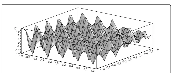
The graph of the Green’s function is displayed in Figure  and Figure  for two diﬀerent values of the spectral parameter.

Figure 1 The graph of the Green’s functionG(x,t,μ) forμ= 3.

(10)

Competing interests

The authors declare that they have no competing interests.

Authors’ contributions

The authors contributed equally to this work. The authors read and approved the ﬁnal manuscript.

Author details

1_{Department of Mathematics, Faculty of Arts and Science, Gaziosmanpa¸sa University, Tokat, 60250, Turkey.}2_{Institute of}

Mathematics and Mechanics, Azerbaijan National Academy of Sciences, Baku, Azerbaijan.

Acknowledgements

The authors would like to thank the referees for their valuable comments. This work was supported by the research fund of Gaziosmanpa¸sa University under Grant No. 2012/126.

Received: 18 September 2014 Accepted: 6 January 2015 References

1. Duﬀy, DG: Green’s Functions with Applications. Chapman & Hall/CRC, Boca Raton (2001) 2. Levitan, BM, Sargsyan, IS: Sturm-Liouville and Dirac Operators. Springer, New York (1991)

3. Ao, J, Sun, J: Matrix representations of Sturm-Liouville problems with coupled eigenparameter-dependent boundary conditions. Appl. Math. Comput.244, 142-148 (2014)

4. Likov, AV, Mikhailov, YA: The Theory of Heat and Mass Transfer. Qosenergaizdat, Moscow (1963) (Russian) 5. Tikhonov, AN, Samarskii, AA: Equations of Mathematical Physics. Pergamon, Oxford (1963)

6. Voitovich, NN, Katsenelbaum, BZ, Sivov, AN: Generalized Method of Eigen-Vibration in the Theory of Diﬀraction. Nauka, Moscow (1997) (Russian)

7. Mukhtarov, OS, Demir, H: Coerciveness of the discontinuous initial- boundary value problem for parabolic equations. Isr. J. Math.114, 239-252 (1999)

8. Mukhtarov, OS, Aydemir, K: New type Sturm-Liouville problems in associated Hilbert spaces. J. Funct. Spaces Appl.

2014, Article ID 606815 (2014)

9. Mukhtarov, OS, Yakubov, S: Problems for ordinary diﬀerential equations with transmission conditions. Appl. Anal.81, 1033-1064 (2002)

10. Rasulov, ML: Methods of Contour Integration. North-Holland, Amsterdam (1967)

11. Titeux, I, Yakubov, Y: Completeness of root functions for thermal conduction in a strip with piecewise continuous coeﬃcients. Math. Models Methods Appl. Sci.7, 1035-1050 (1997)

12. Altını¸sık, N: Asymptotic formulas for eigenfunctions of the Sturm-Liouville problems with eigenvalue parameter in the boundary conditions. Kuwait J. Sci. Eng.39, 1-19 (2012)

13. Aydemir, K: Boundary value problems with eigenvalue depending boundary and transmission conditions. Bound. Value Probl.2014, 131 (2014)

14. Aydemir, K, Muhtarov, FS: Modiﬁed Parseval and Carleman equalities for Sturm-Liouville problems with interior singularities. Contemp. Anal. Appl. Math.2(1), 78-87 (2014)

15. Bairamov, E, Ugurlu, E: On the characteristic values of the real component of a dissipative boundary value transmission problem. Appl. Math. Comput.218, 9657-9663 (2012)

16. Chanane, B: Sturm-Liouville problems with impulse eﬀects. Appl. Math. Comput.190(1), 610-626 (2007) 17. Ao, J, Sun, J, Zhang, M: The ﬁnite spectrum of Sturm-Liouville problems with transmission conditions and

eigenparameter-dependent boundary conditions. Results Math.63, 1057-1070 (2013)

18. Tharwat, MM, Bhrawy, AH, Aloﬁ, AS: Approximation of eigenvalues of discontinuous Sturm-Liouville problems with eigenparameter in all boundary conditions. Bound. Value Probl.2013, 132 (2013)

19. U ˇgurlu, E, Bairamov, E: Dissipative operators with impulsive conditions. J. Math. Chem.51, 1670-1680 (2013) 20. Kong, Q, Wang, QR: Using time scales to study multi-interval Sturm-Liouville problems with interface conditions.

Results Math.63, 451-465 (2013)