R E S E A R C H
Open Access
Target coverage through distributed
clustering in directional sensor networks
Md. Mofijul Islam
1, Md. Ahasanuzzaman
1, Md. Abdur Razzaque
1*, Mohammad Mehedi Hassan
2,
Abdulhameed Alelaiwi
2and Yang Xiang
3Abstract
Maximum target coverage with minimum number of sensor nodes, known as an MCMS problem, is an important problem in directional sensor networks (DSNs). For guaranteed coverage and event reporting, the underlying mechanism must ensure that all targets are covered by the sensors and the resulting network is connected. Existing solutions allow individual sensor nodes to determine the sensing direction for maximum target coverage which produces sensing coverage redundancy and much overhead. Gathering nodes into clusters might provide a better solution to this problem. In this paper, we have designed distributed clustering and target coverage algorithms to address the problem in an energy-efficient way. To the best of our knowledge, this is the first work that exploits cluster heads to determine the active sensing nodes and their directions for solving target coverage problems in DSNs. Our extensive simulation study shows that our system outperforms a number of state-of-the-art approaches.
Keywords: Directional sensor networks; Target coverage; Distributed algorithm; Network lifetime; Cluster
1 Introduction
A directional sensor network (DSN) is composed of a large number of directional sensor devices that send sensed-event reports to a sink. Unlike omnidirectional sensors, the directional sensors have limited range of sensing and communication angles. They promote sensing and communication qualities by focusing transmission in one direction and thus enhance the network performance by increasing the sensing quality and reducing interference and fading. Therefore, there has been a great interest in using directional antennas on sensor nodes to improve the network performances. We can use directional sen-sors in several real-world applications like agriculture field monitoring, military surveillance, infrastructure monitor-ing, etc. In such environments, we have a fixed number of targets for which we need a dynamic algorithm which can select the optimal number of active sensor nodes for monitoring the targets. For instance, in an agricultural field, each tree in a fruit garden might be considered as a sensing target, where a huge number of directional sensor
*Correspondence: [email protected]
1Green Networking Research Group, Department of Computer Science and Engineering, University of Dhaka, Dhaka-1000, Bangladesh
Full list of author information is available at the end of the article
nodes is needed to be deployed. Multimedia and smart camera sensors [1] and the sensors that provide sensing through ultrasonic or infrared [2, 3] are widely used direc-tional sensors. The sensing target coverage determines the percentage of targets from which events are reported to the base station. For guaranteed coverage and event reporting, the underlying mechanism must ensure that all targets are covered by the sensors and the resulting net-work is connected. Gathering nodes into clusters might provide a solution to this problem in an energy-efficient way.
The sensing coverage problem has been well studied in omnidirectional sensor networks [4–7]. However, this issue, in directional sensor networks, has newly attracted the research community [8, 9]. The coverage difficul-ties of directional sensor networks include the limited angle of view, working direction, and line-of-sight (LoS) properties. Three types of coverage problems have been investigated in the literature: area coverage [8, 10–13], target coverage [14–17], and barrier coverage [9, 18, 19]. Among those, the target coverage is the most important application in the domain. In [15] and [16], the multi-ple directional cover set (MDCS) problem of organizing the directions of sensors into a group of non-disjoint cover sets for the all the targets in order to extend
the network lifetime has been solved in distributed and centralized ways, respectively. In the distributed greedy algorithm (DGA) [14], the authors addressed the prob-lem of maximum target coverage with minimum number of sensors (MCMS), which is an NP-complete problem. They provide approximate centralized greedy algorithm (CGA) and DGA solutions to the problem. In all the above solutions, either the sink or the individual sensor nodes run the target coverage algorithms in centralized and distributed solutions, respectively. The first cate-gory suffers from communication overheads and is not scalable, while the second one suffers from computa-tion overhead and poor sensing coverage problems. None of them consider the importance of utilizing the cluster heads in minimizing the number of active sensing nodes and determining their directions to maximize the target coverage.
In this paper, we design a target coverage algorithm through distributed clustering mechanism, namely TCDC, for a directional sensor network in an energy-efficient way. At first, we form clusters in the whole network that builds the data communication backbone. For this, each TCDC sensor node calculates its cluster head selection priority (CSP), separately for each com-munication sector, which is a function of the number of neighbor nodes in that sector, its own residual energy, and its distance from the sink node. The sector, in which a node determines it has the highest priority among its neighbors, is selected as its communication sector, and the node declares itself as the cluster head (CH). Later, each CH collects the target coverage information in dif-ferent sensing directions for all of its member nodes and then runs an algorithm to determine the number of active sensing nodes and their sensing directions. We prove that this CH-based solution yields a better result for the prob-lem of maximum target coverage with minimum number of sensing nodes. In this solution model, the computation overheads for each sensor nodes have been transferred to the CH, minimizing the energy consumption significantly, and it increases the scalability of the network.
The main challenge of our work is to design a dis-tributed algorithm for selecting the cluster heads and ensure their proper utilization in enhancing the tar-get coverage in DSNs. Cluster formation in directional sensors is very difficult because of their limited field of views, working directions, and line-of-sight property. Cluster formation includes CH and gateway selection which requires a better technique that guarantees net-work connectivity so that the data of the target coverage could be delivered to the sink properly. Since the sensing antenna for target coverage is also directional, optimiz-ing the active sensoptimiz-ing nodes and their sensoptimiz-ing sectors, through minimizing the sensing redundancy, is also very difficult.
The major contributions of this paper are summarized as follows:
– The novelty of this work lies in designing a CH-based solution model for the problem of maximum target coverage using minimum number of sensor nodes in directional sensor networks.
– The CH-based determination of sensing sectors, for each TCDC active sensing nodes, decreases the communication and computation overheads of energy-constrained sensor devices.
– The CH-based improvement of the number of active sensing nodes in TCDC minimizes the sensing redundancy and maximizes the number of sleeping nodes in the network.
– We also develop efficient schemes for renewal of CHs, sensing nodes, and gateways, thus promoting the balanced energy consumption in the network and thereby increasing the network lifetime.
– The results of performance evaluations, carried out in ns-3 [20], show that our proposed TCDC system achieves better performances compared to
state-of-the-art protocols in terms of the number of active sensing nodes, sensing coverage, standard deviation of residual energy, and network lifetime.
The remainder of the paper is organized as follows. In Section 2, we discuss the state-of-the-art works on tar-get coverage problems in directional sensor networks, and Section 3 presents the network model and assump-tions. In Section 4, we formulate our proposed clustering which is derived from [21], gateway selection, and tar-get coverage algorithms for directional sensor networks, and energy consumption analysis for the network is pre-sented in Section 5. We carry out performance evaluation of the studied algorithms in ns-3 [20] in Section 6, and we conclude the paper in Section 7.
2 Related work
Sensing coverage is a fundamental problem and has aroused great interest from the industrial and academic community. Three types of coverage problem have been investigated: (1) area coverage [8, 10–13, 22], (2) tar-get coverage [14–16, 23, 24], and (3) barrier coverage [9, 18, 19]. The primary research area relates to our work: target coverage using distribute clustering in a directional sensor network. A MAC protocol, namely DCDMAC (Duty Cycle Direction MAC), is proposed in [25].
greedy algorithm (CGA) and distributed greedy algorithm (DGA).
In DGA, all the sensor nodes gather information on the current state and orientation in the network. Using the priority calculated by the number of targets, one sen-sor node selects its sensing sector. Therefore, there is no coordinator to select the sensing sector for the nodes. Besides, they only use the number of targets as a prior-ity for determining the sensing sector. They also provide SNCS (Sensing Neighborhood Cooperative Sleeping Pro-tocol) which helps in the scheduling of the sensor nodes for energy efficiency. Here, they use the residual energy as a priority for scheduling, and all the sensor nodes run the same DGA algorithm again. Thus, this scheduling mechanism incurs much overhead in the network and decreases the network lifetime as well as performance. As there is no coordinator, the number of messages and infor-mation transmission increases and high computational overhead of the sensor nodes has been observed in the network.
The authors of [23] have studied the multiple directional cover set (MDCS) problem. They tried to organize the directions of the sensors into a group of non-disjoint cover sets to extend the network lifetime. One cover set in which the directions cover all the targets is activated at one time. They designed three algorithms—Progressive, Prog-Resd, and Feedback—in order to prolong the network lifetime with fewer cover sets that are more efficient in practice.
The Progressive algorithm used the idea of this paper [16] of omnidirectional networks for the problem of MDCS. They modify the algorithm to solve the prob-lem of MDCS in directional sensor networks. Prog-Resd takes into consideration the residual lifetime of sensors. This algorithm is different from the Progressive algorithm only in the direction selection process. The Feedback algo-rithm finds fewer cover sets since it utilizes the results obtained from the previous iterations and finds a group of cover sets in the last iteration. It generates no more than Kcover sets which also prolong the network lifetime.
The maximal network lifetime scheduling (MNLS) problem is addressed in the work conducted in [5]. The authors investigate a special target coverage problem where each target has a required coverage quality. They consider that the distance between the sensor and the target influences the coverage quality of the target. They proposed two heuristic greedy algorithms (MNLS-H and MNLS-H-T) for this problem. They wanted to organize the directions into non-disjoint cover sets, and one cover set was activated at a time covering all the targets.
In [26], the authors address the priority-based target coverage in a randomly deployed directional sensor net-work. They assume that each target may have different coverage quality requirements. To solve this problem, they propose a learning-automata-based algorithm to organize
the directional sensors into several cover sets in such a way that each cover set can satisfy coverage quality requirements of all the targets, maximizing the network lifetime.
A greedy approximate algorithm for the maximum directional sensor coverage (MDSC) problem is proposed
in [27]. They also propose the MKDSC (maximum K
directional sensor cover) algorithm selecting and assign-ing directions for a subset of K sensors such that the number of covered target points is maximized.
So, there have been many algorithms for target coverage in directional sensor networks, but none of them utilize the cluster head in order to have a solution of the MCMS problem.
Only a few papers consider the cluster formation in directional sensor networks. In [28], the authors proposed an autonomous cluster algorithm (ACDA) for forming a cluster to achieve both connectivity and sufficient cov-erage with directional sensor networks. This ACDA is a randomized distributed algorithm having four phases: phase I: determining the active sensing sectors, phase II: choosing the communication sectors and cluster heads, phase III: selecting the gateways, and phase IV: renew-ing the cluster head and gateway. In the first phase, each sector of a sensor selects a random sector waiting time (SWT) and broadcasts a Hello message at SWT. After receiving each new Hello message, the SWT is decreased and updated. When the SWT becomes zero on a sector, that sector is selected as the active sector for that par-ticular sensor node. In phase II, each sensor initiates a cluster waiting timer (CWT) that is updated with the help of a number of message transmissions in phase I. A sensor node becomes the cluster head, when the random CWT expires (CWT becomes zero) and none of the neighbor-ing sensors are already members of a cluster. Then, this cluster head broadcasts the message to all its active sec-tors so that the neighboring sensor nodes can form a cluster joining to the cluster head. In phase III, the opera-tion of gateway selecopera-tion can be either triggered by cluster heads or initialized by border sensors. There is random gateway waiting time (GWT) which is updated by the number of message receptions in the phase I, and GWT helps to determine the gateway sensor nodes. In the last phase, the re-clustering mechanism is presented. When a cluster head’s energy is below the threshold, the cluster members again generate new waiting times for form-ing new clusters accordform-ing to the procedure in phases I and II.
for selecting the cluster head and gateway. In renew-ing of the cluster head and gateway, the cluster mem-bers select their waiting time and start passing messages. Besides, the number of messages passing in the cluster and gateway selection phase and renewing of the clus-ter and gateway cost a huge energy of the limited batclus-tery power of the sensor nodes. However, we provide a bet-ter algorithm which will consider the residual energy of the sensor and distance from the sink to calculate the cluster head and gateway in directional sensor networks. Moreover, in our renewing of the cluster and gateway process, the existing cluster head will calculate the prior-ity from the cluster members and select the new cluster head and gateway which will minimize the number of messages passing compared to the autonomous cluster algorithm.
Though many target coverage algorithms have been developed, none has introduced the clustering mechanism in order to solve the target coverage problem in directional sensor networks. Our proposed paper considers network connectivity and coverage and reduces redundancy sens-ing in order to improve energy efficiency in a hierarchical network structure using clustering.
3 Network model
We assume a directional sensor network (DSN) composed of a large set of directional sensor nodesN to cover a set ofMtargets in a two-dimensional plane. The sensors are deployed with random distribution. The DSN has a sink node, to which all sensor devices send their sensed data in multi-hop fashion. Each sensorSihas a fixed and known location (xi,yi), determined by GPS or any other localiza-tion method [29]. Each sensor device is uniquely identified by its ID. We also assume that all the directional sensor nodes are homogeneous in terms of the number of sens-ing sectors, the senssens-ing and communication radius, and the initial energyE0. A sensor node can be in theactiveor sleepingstate. When in the sleeping state, a sensor node periodically wakes up and communicates with its cluster head to check the neighbor communication and sensing coverage.
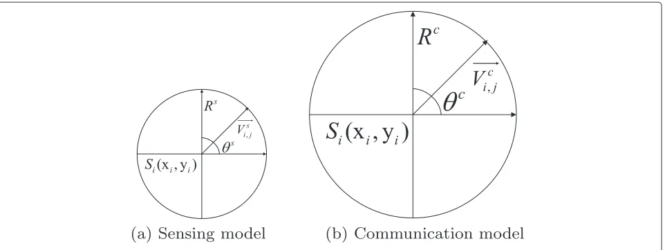
3.1 Directional sensing model
Each sensor has a set of sensing orientations or sectors. We can characterize a sensing sector using the following attributes:
– θs(0< θ <2π): the maximum sensing angle which is called field of view (FOV), as shown in Fig. 1a – Vis,j: the directional vector, which is the center line of
the sensing sector
– Rs: the maximum sensing radius, beyond which a
sensor cannot sense any target. Each sensor knows the locations of the targets within its sensing rangeRs
3.2 Directional communication model
Each sensor also has a set of communication orientations or sectors. We can characterize a communication sector using the following attributes:
– θc(0< θ <2π): the maximum communication angle – Vci,j: the directional vector which is the center line of
the communication sector, as shown in Fig. 1b – Rc: the maximum communication radius, typically,
Rc≥2Rs.
We also assume that each sensor node knows the loca-tion of its neighbor. We adopt the following notaloca-tions throughout the paper:
– N: the set of sensor nodes in the network – Si: theith sensor,1≤i≤N,Si ∈N
– S: the set of sensing sectors of a sensor device
– C: the set of communication sectors of a sensor
device
– nk,wcs: the set of sensor nodes that belong to working communication sector (wcs) of cluster headSk
– Ti,s: the set of targets covered by a sensorSiunder
sectors,Ti,s⊂M
– αk: the set of member sensor nodes of cluster headSk
including the cluster head itself
– SPk: the set of sleeping member nodes of CHSk
Definition 1.A targetTjis covered by sensorSiif and only if the angle betweenSiTjandVi,sin sectorsof sensor Siis within [−θ/ 2,θ/2] andd(Si,Tj)≤Rs.
Definition 2.A sensorSiis neighbor of sensorSjif and only if the angle betweenSjSiandVj,sin sectorsof sensor Sjis within [−θ/ 2,θ/2], andd(Sj,Si)≤Rc.
Definition 3.The working sectors for sensing and com-munications of a sensor are the directions in which it is currently sensing the targets and communicating with the cluster head, respectively.
Fig. 1The directional sensing and communication models.aSensing model andbcommunication model
Definition 5.The network lifetime of a directional sensor network is the time difference from the time of network deployment up to which all the sensors in the network satisfy the following condition:
min ∀i,Si∈N
(Ei) >0. (1)
4 Target coverage through distributed clustering
In this section, we present an energy-efficient solution to the MCMS problem through the distributed clustering mechanism in directional sensor networks. There are four phases in our algorithm:
– Cluster formation. In this phase, cluster heads and communication sectors for each member sensor node are selected. Each sensor nodeSi∈N calculates its CSPi,sin each communication sectors∈C and
determines whether it would be a potential CH for the neighborhood sensor nodes or not.
– Gateway selection. Gateways (GW) are used for inter-cluster communication. Each CHkcalculates GSPi,sin each communication sectors∈Cfor all of
its members inαkand selects a member as the
gateway node having maximumGSPi,svalue to
communicate with the neighbor clusters.
– Target coverage. In this phase, each CHkcalculates TCPi,sin each sensing sectors∈Sfor all of its
members inαkand selects the active sensor nodes and their sensing sectors that cover the targets; the rest of the member nodes go to the low-power sleep state.
– Improvement. Here, we reduce the sensing
redundancy for target coverage that would increase the number of sleeping nodes in the network and thus enhances the network lifetime.
In what follows, we describe in detail the solution components of our proposed target coverage through distributed clustering (TCDC) mechanism. The TCDC exploits single-hop neighborhood information only to solve the MCMS problem. The CHs are taking the com-putation and communication overheads for minimizing the number of active sensing nodes to maximize the cov-erage. Thus, its operation is fully distributed and uses local neighborhood information only, reducing the over-head. Though our solution model cannot be expected to provide a globally optimal solution, it is more computa-tionally scalable and does not incur high communication overhead.
4.1 Cluster formation
At the start of cluster formation phase, each sensor node
Si ∈ N exchanges a neighbor information (NI) message
that consists of its (1) ID, (2) Cartesian location, (3) resid-ual energy, and (4) a set of neighbor sensor nodesni,s in
each communication sector,s ∈ C. Then, each sensor
node calculates cluster head selection priority (CSP) for itself and its neighbors following Eq. 2,
CSPi,s = w1× Ei E0 +
w2× | ni,s| Ni
max
+w3 ×
1−d(Si, SINK) dmax
, ∀s∈C (2)
wherew1,w2,w3are weight factors andw1+w2+w3=1; Nmaxi is determined as
Nmaxi = max ∀s∈C
max ∀j,Sj∈ni,s
max s∈C
(|nj,s|)
,|ni,s|
anddmax is the distance of the sink node from the fur-thest node deployed in the terrain. Thus, it is a system parameter, and its value depends on the size of the terrain and the placement of the sink in the terrain. Since we have assumed static node deployment, the value ofdmax can be computed at the time of node deployments by the sink and each of the sensor nodes can be communicated accordingly. After that, each sensor nodeSi ∈ N checks the following condition:
Now, the following actions will be carried out by the sen-sor devices based on the outcome of Eq. 4 to form clusters throughout the network:
– Action I. If Eq. 4 returns true for any nodeSi∈N, it
declares itself as a CH, fixes its working communication sector accordingly, and starts forming a cluster. This new CH sends a cluster head formation (CHF) message to its neighbors that contains (1) the CH ID, (2) the working communication sector ID, and (3) the set of neighbors in the working communication sector. – Action II. When a sensor nodeSj∈ni,sreceives a
CHF message fromSi, it checks whether it is in the
working communication sector of the new cluster headSi. If yes, it selects its working communication
sector facing towardSiand sends a target coverage
information (TCI) message toSi; it also broadcasts a
cluster membership (CM) message to its single-hop neighbors. Otherwise, a sensor nodeSjupdates CSP
for itself and its neighbors in all sectors following Eq. 2. Note that the TCI message from a cluster member node consists of its (1) ID, (2) CH ID, and (3) the set of covered targets in each sector; also, the CM message consists of the (1) sensor ID and (2) cluster ID.
– Action III. When a sensor node receives a CM message, it updates CSP for itself and its neighbors in all sectors following Eq. 2.
The pseudo-code of the cluster formation procedure is presented in Algorithm 1. An illustrative example of the cluster formation procedure is depicted in Fig. 2. Suppose sensorAhas the highest CSP among its neighbors and it creates a cluster with member sensorsBandC. Similarly, sensorEalso creates a cluster with member sensorsFand G. But sensorDhas no free neighbors, and thus, it creates a single node cluster.
Algorithm 1Cluster head selection, at each sensorSi INPUT: Neighbor information (NI)
OUTPUT: Cluster formation and working communi-cation sector selection.
6: Sisetmas working communication sector
7: Sibroadcasts CHF in all sectors,s∈C
8: exit
9: else if(Receive CHF from any CHSk)then
10: s←{Working communication sector ofSk
11: if(Si∈nk,s)then
12: m←{ sector id ofSi, whereSk ∈ni,m}
13: Sisetsmas working communication
sec-tor
14: Sisends TCI message toSk
15: Sibroadcasts CM in all sectors,s∈C
16: exit
17: else
18: Siupdates NI and CSP values
19: end if
20: else if(Receive CM message)then
21: Siupdates NI and CSP values
22: end if
23: end while
The worst case complexity of Algorithm 1 (cluster
head selection) for a sensor node Si ∈ N is
com-puted as O(|nj,s| × |C|),∀s ∈ C where, ni,s is the
set of neighbor sensor nodes of Si ∈ N in
direc-tion s ∈ C. This is because the sensor Si ∈
N experiences the highest computation penalty if it
declares itself as CH or member of any other CH at last.
4.2 Gateway selection
Fig. 2An example of cluster formation.aBefore cluster formation andbafter cluster formation
GSPi,s = w1× Ei E0+
w2×
|noci,s| Ni
max
+w3×
1−d(Si, SINK) dmax
, ∀s∈C, (5)
wherew1,w2,w3are weight factors andw1+w2+w3=1. Now, a CHSkselects a sensor nodeSias a gateway nodeif and only if the node satisfies the following condition:
max ∀s∈C
(GSPi,s) > max ∀j,Sj∈nk,wcs,j =i
max s∈C
(GSPj,s)
, (6)
where nk,wcs is the set of sensor nodes that belong to the working communication sector (wcs) of cluster head Sk. Thus, a CH Sk selects the most optimal gate-way nodeSi using single-hop neighborhood information and lightweight computations. After that, CHSk broad-casts a gateway selection (GS) message in its working communication sector which is a two-tuple message:
< Gateway Id, Gateway Sector Id >. Note that Eq. 5 is a linear combination of three submatrices—energy, num-ber of neighbor nodes of other clusters, and distance to the sink node. Thus, in selecting a gateway node, the CH maximizes the node’s residual energy and the num-ber of neighbor nodes of other clusters, and minimizes its distance to the sink node.
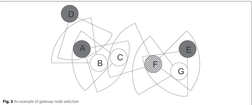
An example of the gateway selection process is described below using Fig. 3. Suppose a sector of sensorF has the highest GSP than other members of CHE. There-fore, the nodeFis selected as the gateway for this cluster that can communicate with sensorC, which is a member
of CHA. However, CHDhas no member sensor nodes
that can be used as gateway; it can directly communicate with CHAusing an appropriate communication sector.
In the process of solving the MCMS problem in our pro-posed TCDC system, we now exploit each CH to select the sensor nodes and their active sectors for target coverage.
Therefore, our proposed Algorithm 2 for target cover-age (to be presented in Section 4.3) can be executed only when the clusters are formed throughout the network by executing Algorithm 1.
4.3 Target coverage
The novelty of our proposed TCDC system is to solve the target coverage problem using the knowledge acquired by the cluster heads. Each CH translates the target cover-age problem into determining optimal sensing sectors for its member nodes so that all targets can be covered by a
minimum number of sensing nodes. A CHSkcomputes a
target coverage priority (TCP) metric for all of its member nodes inαkfor all sensing directionss∈Sas follows:
TCPi,s=c1× Ei E0 +
c2× | Ti,s| Tk
max
, ∀s∈S (7)
wherec1andc2are the weight factors for target coverage prioritization andc1+ c2 = 1;Ti,s is the set of targets covered by a sensorSiin sensing directions, andTmaxk is the maximum number of targets covered by any member sensor node of CHSkand it is determined as follows:
Tmaxk = max ∀i,Si∈nk,wcs
max s∈S(|
Ti,s|)
. (8)
Note here that for computing TCP of member nodes, each CH exploits only local information—member node’s residual energy (Ei) and their target coverage information (TCI), acquired during cluster formation, as discussed in Section 4.1.
Then, a CH Sk determines a sensing node Si and
its working sensing sector that satisfies the following condition:
max ∀s∈S
(TCPi,s) > max ∀j,Sj∈nk,wcs,j =i
max s∈S
(TCPj,s)
, (9)
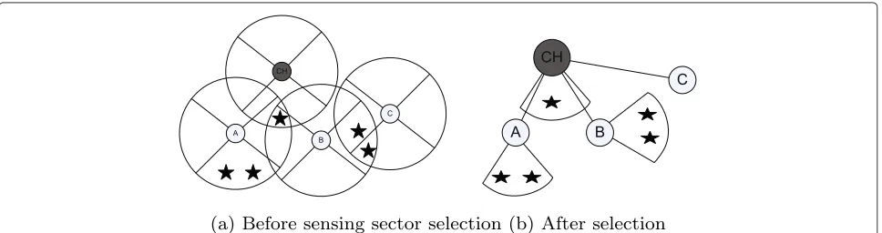
wherenk,wcsis the working communication sector of CH Sk. Then, CH Sk sends a sensing sector selection (SSS) message to the selected member nodeSi so that the lat-ter can set its sensing direction accordingly, as stated in line no. 14 of Algorithm 2. In the meantime, the CH
updates TCP, using Eq. 7, for the updated set of member nodes,αk, and target setTi,s, as stated in line nos. 4–10 in Algorithm 2. Thus, our target coverage algorithm runs untilαk becomes null or all the targets are covered. After that, the CH sends a Sleep message (SM) to the rest of the member sensor nodes that are neither responsible for covering any target nor selected as gateway, as stated in line nos. 12–19 of Algorithm 2, which helps to prolong the network lifetime. As shown in Fig. 4, the sensing sectors
of the CH and the two member sensor nodesAandBare
determined to cover all the five targets, and the node C goes to sleep mode.
Algorithm 2 Target coverage algorithm, at each cluster headSk
INPUT: Cluster member nodes and target coverage information.
OUTPUT: Active sensing nodes and their sensing sectors.
1: while(αk = ∅AND maxSj∈αk,s∈S |Tj,s| =0)do
2: Select a sensorSiand its sectormusing Eq. 9
3: αk ←αk− {Si}
4: for allSj∈αkdo
5: for alls∈Sdo
6: Tj,s←Tj,s−Ti,m
7: Update priority TCPj,susing Eq. 7
8: end for
9: end for
10: Send the SSS message to sensorSito set its working sensing sectorm.
11: end while
12: if(|αk|>0)thenSend all other nodes in sleep mode
13: for allSj∈αkdo
14: if(Sjis not a gateway node)then
15: CH sends a Sleep message toSj
16: SensorSjwill go to sleep mode
17: end if
18: end for
19: end if
The complexity of Algorithm 2 (target coverage algo-rithm) is computed asO(|αk|2× |
S|). This is the worst case complexity of target coverage algorithm of each CH in the network, when all of its member sensor nodesSi∈ αk are selected as active sensing nodes. Furthermore, the best case complexity isO(|αk| × |S|); it happens if all the targets are covered by activating a single sensor node Si∈αkonly.
Theorem 1. The proposed TCDC system creates an opti-mal cover set for each cluster.
Proof.We use proof by contradiction. Assume that the TCDC system does not choose the local optimal cover set Ok, i.e.,∃Skthat selects a cover setCkwhereCk ⊂Ok.
To determine the nodes in a cover set, each cluster head Sk calculates TCP for ∀Si ∈ αk and creates a set A= {s1,s2,s3,. . .sn|n = |αk|and TCP(s1) > TCP(s2) > TCP(s3) . . .TCP(sn−1) >TCP(sn)}. The CH then selects the first node from this sorted list and updates the TCP values for all other nodes, then sorts them again. This process continues until all targets are covered or there remains any member node, which is not yet selected. Therefore, the TCDC system ensures that there will be no other possible optimal cover setCkfor any cluster headSk in terms of target coverage and network lifetime, captured by the measurement of TCP values. But it contradicts our initial assumption.
4.4 Improvement
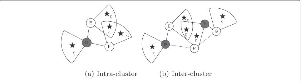
One of the major limitations of our target coverage algo-rithm, described in Section 4.3, is that a target can be covered by multiple sensor nodes, and thus, redundant sensed data will be sent to the sink, causing wastage of bandwidth and energy. This redundant sensing can be found within the members of one cluster or neighbor clusters, as illustrated in Fig. 5. In Fig. 5a, the targetT3
is sensed by two sensor nodes E and F, and both are
members of cluster headD; hence, it is an intra-cluster duplicate coverage issue. Figure 5b shows that the target T3is covered by sensor nodesEandF, and now they are
members of different cluster headsDandG. Therefore, it causes an inter-cluster duplicate coverage problem. In this section, we design a mechanism that reduces redundant data flow to the sink.
The intra-cluster duplicate coverage problem is solved as follows. At first, a cluster head finds the targets that are covered by multiple sensing nodes. Then, for each such target, it searches for the corresponding sensing node that has the highest TCP value, which will be responsible for covering the target, and the rest of the lower pri-ority sensing nodes will be in the block list for that target. Thus, the CH can produce a block list table, < Blocked sensor node ID,Target ID(s) >, for all the block listed sensor nodes. Now, for each block listed sensor node, the CH checks whether the total number of targets covered by the sensor is equal to the total number of tar-gets for which it is block listed. If yes, the CH sends a SM to that node for energy saving; otherwise, it sends a block list (BL) message (containing the target ID(s)) to that sen-sor node so that the latter can ignore sending data for that target.
The solution to the inter-cluster duplicate coverage problem necessitates the neighbor clusters to exchange their CSP values, member list, target IDs covered by the members, and their TCP values. Following the same pro-cedure used in the intra-cluster duplicate coverage prob-lem, each CH determines the sensor nodes that can go to sleep mode and ignores sending data for a specific target. If the TCP values of the member nodes in differ-ent clusters, which have duplicate coverage, are the same, then the conflict resolution works as follows: the CH having a lower CSP value performs the further actions. Thus, our proposed TCDC system would save a signifi-cant amount of energy and network bandwidth wastage through lightweight improvements.
4.5 Periodic scheduling of nodes
In this section, we present re-scheduling of cluster heads, gateways, and sensing nodes to prolong the network life-time.
4.5.1 Cluster head renewing
When the residual energy of a cluster head Sk, REk, becomes lower than a predefined threshold value REkth, i.e., REk < REkth, then the CH collects neighbor infor-mation (NI) from its member nodes to elect a new CH. Then, it calculates CSP for each of its member nodes and thus selects a new CH Si, which satisfies the following condition:
max ∀s∈C(
CSPi,s) > max ∀j,Sj∈nk,wcs,j =i
max ∀s∈C(
CSPj,s)
. (10)
In case the newly formed cluster head does not cover all the existing members, another CH may need to be selected, following the same procedure. The old CH now becomes an ordinary member sensing node and updates its energy threshold as follows: REkth = 12REkth. This is done to decrease the possibility of taking the responsi-bility CH by the same node again. Therefore, the energy load distribution among the network nodes will be more balanced.
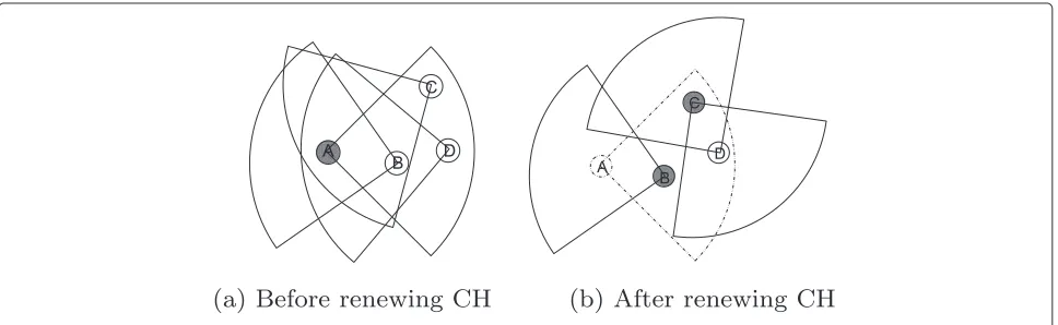
For example, in Fig. 6a, when the residual energy of clus-ter headAbecomes less than a predefined threshold, the renewal process of CH starts and two new clusters are formed (CHCand CHB), as shown in Fig. 6b.
Also, note that in the renewal process of cluster heads in our proposed TCDC system for directional sensor net-works, we do not run the cluster formation Algorithm 1 in all the member nodes. The old cluster head collects NI information from the member sensor nodes and handover the CH responsibility to another node(s). Furthermore, the above CH renewing process decreases the communi-cation and operation overheads through using localized information and computation. Thus, it does not incur much more energy overheads.
To ensure the coverage of the targets of the incumbent region, where new CH(s) has been formed, the proposed TCDC system locally runs the gateway selection mech-anism, target coverage algorithm (Algorithm 2), and the coverage redundancy minimization phases. The above
process may include the coverage of any unattended tar-gets or lose a target covered by the previous clusters. Thus, it is expected that the members of the new CH(s) would retain a good level of target coverage in the changed region.
4.5.2 Sensing node scheduling
The residual energy of the cluster member nodes may also go below the threshold value. In that case, it sends a message to its cluster head requesting to select a new member from the sensors that are in sleep mode. The CH will search for the replacement of the dying node from the member nodes in the sleeping mode using Eq. 9.
4.5.3 Gateway renewing
If the residual energy of the gateway node becomes less than the threshold value, it sends a message to the cluster head to select a new gateway in the same way as described in Section 4.2.
4.6 Discussion
In this section, we discuss on the parameter selection and weight factors in Eqs. 2, 5, and 7.
4.6.1 Parameter selection
The rationale to define the aggregated weight function in Eq. 2 is to maximize CSP, which is a linear combination of three parameters. The first parameter of Eq. 2 denotes how much fraction of the residual energy is remaining over the initial energy, the second parameter represents the density of the neighbor nodes, and the third param-eter is corresponding to the distance of a sensor node from the sink. Thus, the maximization of the linear sum of these three parameters for different sensors (see Eq. 4) guarantees that a node will be selected as a CH having higher residual energy, greater number of cluster mem-bers, and reduced hop count to the sink. Similarly, in Eq. 5, the number of neighbor sensor nodes of different clus-ters has been considered (see the second parameter) that ensures better selection of a gateway node for inter-cluster
communication. Also, in Eqs. 7 and 9, the maximization of the second parameter increases the target coverage percentage. The performances of the aggregated priority metrics, derived from Eqs. 2, 5, and 7, are largely depen-dent on the values of the chosen weight factors, which we discuss below.
4.6.2 Weight factors
Setting appropriate values for the weight factors w1,w2,w3,c1, and c2 is very important for achieving optimal solutions to clustering and coverage problems that we have addressed in this work. The weight fac-tors correspond to complex multivariable functions, and their optimal values are dynamic depending on the time-varying network environment parameters. Therefore, the problem can be modeled as a simulation optimization problem, where the objective function cannot be eval-uated exactly. Adaptive random search methods for the simulation optimization problem, which can maintain balance among exploration, exploitation, and estimation, are more effective [30, 31]. However, the development of an adaptive and almost surely convergent search method for our problem leads to a new research work. Therefore, we have gone for the estimation based on performing a lot of simulation runs (transient simulation) for a sub-stantially longer period of time. We run our simulations for different values of these weight factors, network size, node density, and initial node energy. The experiments state that the following values for the weight factors increase the overall performance of our TCDC system: w1= 0.45,w2 = 0.35,w3= 0.20,c1 = 0.6, andc2 =0.4, determined through numerous simulation runs for dif-ferent network size, node density, and initial node energy values as in [32].
5 Energy consumption analysis
This section presents energy consumption analysis in each phase of the proposed TCDC system. We assume that the energy needed to transmit and receive a message of 1 bit for each sensor with omnidirectional antennas isET and ER, respectively. Thus, the energy consumption to trans-mit a 1-bit message for a directional sensor is calculated as ET
|C|.
The transmission energy of a node that covers a neigh-borhood of radiusRcis given by
ET=max{ET[ min] ,ETA×(Rc)α} +ETE (11)
whereETEis the energy per bit needed by the transmitter electronics,ETAis the energy consumption of the trans-mitting amplifier to send 1 bit over one unit distance, and
α(1.6≤α≤0.6)is the path loss factor depending on the radio frequency environment. For all nodes closer than
Rcmin =
, the energy requirement is constant
at ET[ min] J/b. Typical values of these parameters are ET = 50 nJ/b,ER = 50 nJ/b, andETA = 0.0013 nJ/b/m4 whenα = 4 [33]. The energy per bit needed by receiver electronics is typicallyER = ERE = 50 nJ/b. There is no difference between listening and receiving in this radio transceiver model.
5.1 Cluster formation
In the cluster formation phase, every sensor node broad-casts an NI message in all its communication sectors,C. Thus, the total number of NI messages transmitted in this phase is calculated as NTNI
CF = |C| × |N|. In the same way, each sensor receives a message from all of its neighbors in each sectors, and thus, the total number of NI messages received throughout the network isNRCFNI =
|N| i=1
|C|
s=1 |ni,s|, where|ni,s|is the number of neighbors of sensor Si in direction s. After selecting the working communication sector, each CH broadcasts a CHF mes-sage in all sectors, and thus, the total number of CHF transmissions isNTCHF
CF = |C| × |CH|, where CH is the set of CHs formed, and the corresponding total num-ber of receptions isNRCHF
CF =
|N|
i=1|s=1C||NCHi,s|, where NCHi,sis the set of neighbor CHs of sensorSiin sectors. After that, each member node of a CH broadcasts a CM message in all its sectors. Therefore, the total number of CM message transmissions isNTCFCM = |C| × |N −CH|
and that of receptions isNRCFCM=Si∈(N−CH)s|=1C||ni,s|. Thus, the total amount of energy consumption in the cluster formation phase is calculated as
EtotalCF = ET CHF, and CM messages in bits, respectively.
5.2 Gateway selection
Each CH selects a gateway for inter-cluster communica-tion, and it broadcasts a gateway selection (GS) message to its members. The total number of GS messages for transmission isNTGS
GW = |CH| and that for reception is amount of energy consumption in this phase is calculated as
5.3 Target coverage
In this phase, each cluster member sends a TCI mes-sage to its cluster head, and thus, the total number of TCI messages transmitted isNTTCI
TC = (|N| − |CH|)and that received is NRTCI
TC =
Sk∈CHαk. After a CH
deter-mines the active sensing sector for its member nodes, it sends an SSS message to them. The number of SSS mes-sages transmitted is NTSSS
TC = |CH| and that received is amount of energy consumption in this phase is calculated as
5.4 Renewing of CHs, GWs, and sensing nodes
The periodic scheduling part of TCDC, stated in Section 4.5, runs only in the CHs, to renew cluster heads and gateways, and to change the operation states of sens-ing nodes. In this phase, the old CH first notifies its members to send NI messages. The total number of NI messages transmitted to CH is NTNI
rch = |αk| and that of reception is NRNI
rch = |αk|. Once a new CH Sk is determined, it broadcasts a CHF message in its work-ing communication sector. Therefore, the total number of CHF message transmissions and receptions is calculated asNTCHF
rch =N CHF
Rrch = |αk|. Thus, the total amount of energy consumption in renewing one cluster is calculated as
Etotalrch = ET
As stated in Section 4.5, when renewing a gateway node, a cluster headSkcollects NI messages from all of its mem-bers, determines the new gateway, and broadcasts a GS message in its working communication sector. Thus, the total number of NI and GS message transmissions is cal-culated as NTrgw = |αk| + 1 and that of reception is NRrgw = 2× |αk|. Therefore, the total amount of energy consumption to renew a gateway is calculated as
Etotalrgw = (|NI| + |GS|)×
For renewing the state of a sensing node, the cluster headSkcollects TCI messages from the sleeping member nodes during their wake-up intervals. Therefore, the total number of TCI message transmissions isNTrssTCI = |SPk|, where SPk is the set of sleeping member nodes in CHSk,
and that of reception is NRrssTCI = |SPk|. After that, the CH broadcasts an SSS message to its member nodes, as stated in Section 4.5. Thus, the total number of SSS mes-sage transmissions is NTrssSSS = 1 and that of receptions is NRrssSSS = |αk|. Therefore, the total amount of energy consumption to renew a sensing node is calculated as
Ersstotal = ET
The above discussion helps form a mathematical model on the total number of transmitted and received messages and the corresponding analysis of energy consumption in the network.
6 Performance evaluation 6.1 Simulation environment
We evaluate the performances of our proposed TCDC system in ns-3 [20], a discrete-event network simulator, and compare the results with two state-of-the-art works: autonomous clustering via directional antenna (ACDA) [28] and distributed greedy algorithm (DGA) [14]. We
deploy the sensors and targets in a region of 1000 ×
1000 m2 with randomly uniform distribution. The
net-work configuration parameters are shown in Table 1. For each graph points, we run 100 simulation runs and take the average of the results.
6.2 Performance metrics
We have considered the following performance metrics for studying the effectiveness of our proposed TCDC system.
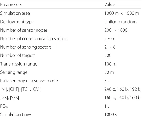
Table 1Network configuration parameters
Parameters Value
Simulation area 1000 m×1000 m
Deployment type Uniform random
Number of sensor nodes 200∼1000
Number of communication sectors 2∼6
Number of sensing sectors 2∼6
Number of targets 200
Transmission range 100 m
Sensing range 50 m
Initial energy of a sensor node 5 J
|NI|,|CHF|,|TCI|,|CM| 240 b, 160 b, 192 b,
|GS|,|SSS| 160 b, 160 b, 160 b
REth 1 J
– Number of cluster heads. We measure the number of cluster heads formed during the clustering algorithm in all the studied protocols, i.e., it represents the number of clusters in the network. The less number of clusters in the network corresponds to the reduced operation overhead.
– Number of active sensing nodes. We measure the
number of active sensing nodes that are required to cover all the targets in the terrain. The less the value is, the more number of sensor nodes can go to sleep mode and conserve energy.
– Target coverage. The target coverage percentage is measured as the ratio of the number of covered targets to the total number of targets deployed in the terrain. The target coverage is the most important issue in the directional sensor network, and thus, the higher percentage of coverage is expected.
– Standard deviation of energy. The standard deviation of energy defines the average variance between the residual energy levels on all nodes and is measured by Eq. 18,
whereEiandμare, respectively, the residual energy
of nodeSiand the mean residual energy for all nodes.
Therefore, the value ofσindicates how well the energy consumption is distributed among the sensor nodes. The smaller the value is, the better is the capability of the TCDC system to balance the energy consumption.
– Network lifetime. Please refer to Definition 5 in Section 3.
6.3 Simulation result
We study the performances for varying the number of sensor nodes deployed in the network and the number of sensing and communication sectors to evaluate the robustness of our proposed TCDC system in different environments. ACDA does not solve the target coverage problem; rather, it solves the area coverage problem, and thus, we do not compare its performance with TCDC with respect to the number of targets covered. Similarly, we cannot compare the performance of our TCDC algorithm with that of DGA for the number of CHs formed since the latter does not implement the clustering mechanism.
6.3.1 Impacts of number of sensor nodes
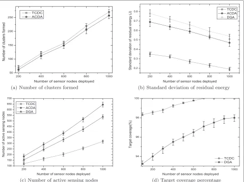
We measure the performance metrics discussed before for varying the number of directional sensor nodes ranging from 200 to 1000, at an interval of 200 nodes; the number of sectors is kept at 3, and the total number of fixed target is 200.
The graphs in Fig. 7a show that the number of clus-ters formed increases with the number of deployed sensor nodes both in ACDA and TCDC. In ACDA, a bit reduced number of clusters is formed compared to our TCDC system since the former considers two-hop neighbors as cluster members. Even though the number of formed clusters is more in our TCDC system, its communica-tion overhead for cluster maintenance, renewing CHs, and gateways, etc. will be much lower compared to that of the ACDA system due to its consideration of one-hop cluster members.
Figure 7b shows the standard deviation of residual energy levels for increasing the number of sensor nodes deployed in the network. The graphs depict that the stan-dard deviation of the residual energy of nodes decreases with the increasing number of nodes deployed in the network since the latter increases the opportunity of get-ting alternate nodes (having higher residual energy) in the neighborhood that can work as an ordinary sensor or gate-way or even as a CH. Our proposed TCDC system gives much better performance than both the ACDA and DGA algorithms. TCDC shows better performance than ACDA because of two reasons: first, ACDA does not consider the residual energy level of nodes when selecting CHs, gateways, and active sensing nodes, and thus, it increases unbalanced energy consumption;second, dynamic update of the residual energy thresholds for selecting/renewing CHs in our TCDC system helps it to ensure balanced energy consumption. On the other hand, the poor selec-tion of active sensing nodes and inefficient mechanism of rescheduling of sensor nodes without having a coor-dinator are the main reasons why our proposed TCDC algorithm gives better result than DGA.
Fig. 7Impacts of number of sensor nodes.aNumber of clusters formed.bStandard deviation of residual energy.cNumber of active sensing nodes. dTarget coverage percentage
communication sector of the sensor nodes with the help of CHs and better rescheduling mechanism of CHs and gateways increases the number of sleep nodes in TCDC compared to the ACDA algorithm. Therefore, a substan-tial performance improvement by our TCDC system has been achieved.
Figure 7d reveals that a substantial improvement in terms of target sensing coverage percentage has been achieved by our TCDC algorithm compared to DGA. Our algorithm shows better performance because the CH takes the responsibility of being a coordinator, aggregates the target coverage information (TCI) from the mem-ber sensor nodes, and optimizes the best sensing sec-tor for the sensor nodes. Here, a CH has all the target information (that are covered by its member nodes) and runs the target coverage algorithm as a centralized entity, and thus, it can take the most optimal decisions. The graphs in Fig. 7d show that our algorithm reaches almost 100 % target coverage when the number of deployed
sensor nodes increases to 700. It is also evident from all the graphs of Fig. 7 that the confidence interval of our proposed TCDC system is much lower compared to that of the DGA and ACDA systems, i.e., the TCDC system shows better performance stability compared to them.
Fig. 8Impact of number of sensor nodes on network lifetime
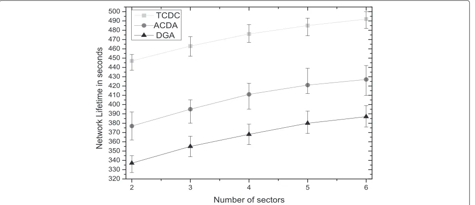
6.3.2 Impacts of number of sectors
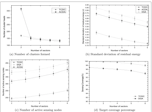
In this section, we evaluate the impacts of the number of communication and sensing sectors, ranging from 2 to 6, of the sensor devices on the performances of the studied algorithms. In this experiment, we have fixed the number of sensor nodes deployed in the area at 600 and the total number of targets is 100.
Figure 9a shows the impact of the number of sectors on cluster formation. The graphs show that when the number of sectors is two, the ACDA algorithm forms almost double number of clusters compared to our TCDC algorithm. The reason behind this is that in this case, the random waiting timer used in ACDA is decreased (due to the increased number of neighborhood nodes) for selecting the active communication sector and the cluster head, and thus, the number of members in each cluster is reduced. But the ACDA algorithm forms a bit reduced number of clusters as the number of sectors increases from three to six. Our in-depth look into the simulation trace file reveals that even though the number of formed clusters is a bit more in our TCDC system, its com-munication overhead for cluster formation and renewing CHs and gateways, etc. is much lower compared to the ACDA system due to its consideration of one-hop cluster members.
The graphs in Fig. 9b state that the standard devia-tion of residual energy level decreases slowly with the increasing number of sectors for ACDA, DGA, and TCDC algorithms. Our proposed TCDC system gives much bet-ter performance than the ACDA and DGA algorithms. As stated in Section 6.3.1 for the number of sensors, the larger number of sectors also increases the number of options from which the CH can choose the optimal one
based on priority. Therefore, the energy load will be dis-tributed on many nodes sparsely, reducing the standard deviation.
The number of active sensor nodes is increased with the number of sectors, as depicted in Fig. 9c. However, in our TCDC algorithm, almost 15 and 25 % less number of sens-ing nodes remain active compared to the ACDA and DGA algorithms, respectively. This happened due to the follow-ing reasons: cluster formation helps the sensor nodes to be coordinated by the CHs, and CHs select the best cover set in solving the MCMS problem. The efficient selection of the communication sectors and the rescheduling mech-anism of the cluster head and gateway nodes increase the performance of our proposed algorithm. Besides, the solu-tion to duplicate the coverage problem in TCDC helps it to send a good number of sensor nodes to the sleep state, reducing the active sensing nodes.
Figure 9d states that the target sensing coverage per-centage in both TCDC and DGA slightly decreases with the number of sensing sectors. The increasing number of sectors decreases the number of targets covered by each sector (due to the decreased view of the angle), i.e., the number of targets per sensor is decreased for the whole network, which in turn decreases the probability that a target will be covered by at least one sensor in the net-work. The graphs also state that our TCDC algorithm performs better than the DGA algorithm despite the increasing number of sectors. In our TCDC system, the CHs run the target coverage algorithm that determines the active sensor nodes and their sensing directions, yield-ing an optimal cover set for target coverage.
The comparison of network lifetime offered by TCDC, ACDA, and DGA algorithms is shown in Fig. 10 for
Fig. 11Impacts of sensing and communication ranges.aNumber of active sensing nodes.bTarget coverage percentage
increasing number of sectors. As expected theoretically, the network lifetime linearly increases with the num-ber of sectors for all the studied protocols since it increases the options of choosing an optimal node based on priority. The other causes are already explained in Section 6.3.1.
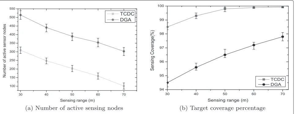
6.3.3 Impacts of sensing range
We have also studied the comparative performances for varying sensing ranges. In this experiment, we have deployed 600 sensor nodes in the network, each having three sensing and communication sectors. The communi-cation ranges are also increased with the sensing ranges proportionately, i.e.,Rc = 2×Rs. The impact of varying sensing range on active sensor nodes is shown in Fig. 11a. Increasing the sensing range decreases the active sensor nodes on both the TCDC and DGA algorithms; however, our TCDC system provides more than 50 % performance improvement when the sensing range is doubled (from 30 to 60 m). Figure 11b shows that the sensing coverage increases with the sensing range in both the algorithms, as expected theoretically. While the proposed TCDC sys-tem achieves closer to 100 % coverage with the 50 m and above sensing range, the DGA can reach closer to 98 % with the 70 m range and this is caused by non-coordinated selection of sensing nodes and their sectors.
7 Conclusions
This paper has presented a CH-based distributed target coverage algorithm in directional sensor networks. The proposed TCDC system is the first approach to address the MCMS problem using cluster heads. In the TCDC sys-tem, the CHs and gateways are determined first, and then each CH co-ordinates selection of the active sensor nodes and their sensing directions. This work has also addressed
the duplicate target coverage problem to optimize the net-work performance while increasing the netnet-work lifetime. Our intelligent and energy-efficient solution to the renew-ing procedure of CHs, GWs, and sensor nodes is done by the CHs, exploiting single-hop neighborhood informa-tion only. Therefore, the absence of a global informainforma-tion exchange scheme reduces the network setup and updating costs and alleviates the possibility of incorrect information at the nodes as changes in system topology occur. Our per-formance evaluation results also depict that the proposed TCDC system achieves significant improvement over the state-of-the-art techniques in terms of target coverage, network lifetime, etc.
Although the proposed system achieves better perfor-mance, further experimental and theoretical extensions are possible. The weight factors in our system need a bet-ter mathematical analysis for dynamically selecting their values, and we have left it for our future work.
Competing interests
The authors declare that they have no competing interests.
Acknowledgements
The authors would like to extend their sincere appreciation to the Deanship of Scientific Research at King Saud University for its funding of this research through the Research Group Project no. RGP-VPP-281.
Author details
1Green Networking Research Group, Department of Computer Science and Engineering, University of Dhaka, Dhaka-1000, Bangladesh.2Information Systems Department, College of Computer and Information Sciences, King Saud University, Riyadh 11543, Kingdom of Saudi Arabia.3School of Information Technology, Deakin University, Burwood, VIC 3125, Australia.
Received: 3 October 2014 Accepted: 20 May 2015
References
2. M Emanuele, Z Andrea, Z Stefano, Z Francesco, P Enrico, inProceedings of the 2009 IEEE International Conference on Robotics and Automation, ICRA’09. Range-only SLAM with a mobile robot and a wireless sensor networks (IEEE Press Piscataway, NJ, USA, 2009), pp. 1699–1705 3. S Robert, M Alan, P Joseph, A John, C David, inProceedings of the 2nd
International Conference on Embedded Networked Sensor Systems,SenSys ’04. An analysis of a large scale habitat monitoring application (ACM New York, NY, USA, 2004), pp. 214–226
4. L Hai, Peng-W Jun, Y Chih-Wei, J Xiaohua, SAM Makki, P Niki, inINFOCOM, Miami, Florida, USA, 13–17 March 2005. Maximal lifetime scheduling in sensor surveillance networks (IEEE, 2005), pp. 2482–2491
5. C Ionut, C Mihaela, Energy efficient connected coverage in wireless sensor networks. Int. J. Sen. Netw.3(3), 201–210 (2008)
6. W Bang, Coverage problems in sensor networks: a survey. ACM Comput. Surv.43(4), 32:1–32:53 (2011)
7. M Seapahn, K Farinaz, P Miodrag, BS Mani, Senior Member. Worst and best-case coverage in sensor networks. IEEE Trans. Mobile Comput.4, 84–92 (2005)
8. B Xiaole, K Santosh, X Dong, Y Ziqiu, HL Ten, inProceedings of the 7th ACM International Symposium on Mobile Ad Hoc Networking and Computing, MobiHoc ’06. Deploying wireless sensors to achieve both coverage and connectivity (ACM, New York, NY, USA, 2006), pp. 131–142
9. W Yi, C Guohong, inProceedings of the Twelfth ACM International Symposium on Mobile Ad Hoc Networking and Computing,MobiHoc ’11. Barrier coverage in camera sensor networks (ACM New York, NY, USA, 2011), pp. 12:1–12:10
10. SK Gaurav, B Yigal, S Saswati, inProceedings of the 15th Annual International Conference on Mobile Computing and Networking,MobiCom ’09. Lifetime and coverage guarantees through distributed coordinate-free sensor activation (ACM, New York, NY, USA, 2009), pp. 169–180
11. M Huadong, Z Xi, M Anlong, inINFOCOM,Rio de, Janeiro, Brazil. A coverage-enhancing method for 3D directional sensor networks (IEEE, 2009), pp. 2791–2795
12. Y Zuoming, T Jin, B Xiaole, X Dong, J Weijia, inProceedings of IEEE INFOCOM. Connected coverage in wireless sensor networks with directional antennas (Shanghai, China, 10), pp. 2264–2272 13. S Selina, NN Fernaz, R Abdur, R Mustafizur, inInt’l Conf on Networking
Systems and Security (NSysS),Dhaka, Bangladesh. Network life time aware area coverage for clustered directional sensor networks (IEEE, 2015), pp. 1–9
14. A Jing, AA Alhussein, Coverage by directional sensors in randomly deployed wireless sensor networks. J. Comb. Optimization.11, 21–41 (2006)
15. C Yanli, L Wei, L Minglu, L Xiang-Yang, Energy efficient target-oriented scheduling in directional sensor networks. IEEE Trans. Comput.58(9), 1259–1274 (2009)
16. C Mihaela, TT My, L Yingshu, W Weili, inProceedings of IEEE INFOCOM. Energy-efficient target coverage in wireless sensor networks (Miami, Florida, USA, 13), pp. 1976–1984
17. Z Qun, G Mohan, Lifetime maximization for connected target coverage in wireless sensor networks. IEEE/ACM Trans. Netw.16(6), 1378–1391 (2008) 18. C Ai, K Santosh, HL Ten, inProceedings of the 13th Annual ACM
International Conference on Mobile Computing and Networking,MobiCom ’07. Designing localized algorithms for barrier coverage (ACM New York, NY, USA, 2007), pp. 63–74
19. K Santosh, Hwang Ten-L, A Anish, Barrier coverage with wireless sensors. Wireless Netw.13(6), 817–834 (2007)
20. Institute Information Sciences, NS-3 network simulator. (2008) Software Package www.nsnam.org
21. MM Islam, M Ahasanuzzaman, MA Razzaque, MM Hassan, A Alamri, in Wireless and Mobile, 2014 IEEE Asia Pacific Conference on. A distributed clustering algorithm for target coverage in directional sensor networks (Bali, Indonesia, 28–30 August 2014), pp. 42–47
22. Y Zuoming, T Jin, B Xiaole, X Dong, J Weijia, Connected coverage in wireless networks with directional antennas. ACM Trans. Sen. Netw.10(3), 51:1–51:28 (2014)
23. C Yanli, L Wei, Li X-Y, Li Minglu, inINFOCOM. Target-oriented scheduling in directional sensor networks (IEEE Barcelona, Spain, 2007), pp. 1550–1558 24. E Asma, R Abdur, Mohammad H Mehedi, A Ahmad, A Atif, Moving target tracking through distributed clustering in directional sensor networks. Sensors.14(12), 24381–24407 (2014)
25. N Fernaz Narin, S Selina, R Abdur, I Shariful, inInt’l Conf on Networking Systems and Security (NSysS),Dhaka, Bangladesh. A duty cycle directional MAC protocol for wireless directional sensor networks (IEEE, 2015) 26. M Hosein, S Shaharuddin, AbdulI Samad, A learning automata-based
solution to the priority-based target coverage problem in directional sensor networks. Wireless Personal Commun.79(3), 2323–2338 (2014) 27. L Zaixin, WW L i, inNetworking, Sensing and Control (ICNSC), 2014 IEEE 11th
International Conference on. Approximation algorithms for maximum target coverage in directional sensor networks (Miami, Florida, USA, 7), pp. 155–160
28. Ying-C Chih, Chih-W Yu, Distributed clustering with directional antennas for wireless sensor networks. Sensors J IEEE.13, 2166–2180 (2013) 29. L Kezhong, X Ji, A fine-grained localization scheme using a mobile
beacon node for wireless sensor networks. JIPS.6(2), 147–162 (2010) 30. AA Prudius,Adaptive Random Search Methods for Simulation Optimization.
(Georgia Institute of Technology, Atlanta, Georgia, USA, 2007) 31. JC Spall,Introduction to, Stochastic Search and Optimization: Estimation,
Simulation, and Control. (Wiley, New York, 2003)
32. MM Rashid, MM Alam, MA Razzaque, CS Hong, Congestion avoidance and fair event detection in wireless sensor network. IEICE Trans. Commun. 90(12), 3362–3372 (2007)
33. WB Heinzelman, AP Chandrakasan, H Balakrishnan, An
application-specific protocol architecture for wireless microsensor networks. Trans. Wireless. Comm.1(4), 660–670 (2002)
Submit your manuscript to a
journal and benefi t from:
7Convenient online submission
7Rigorous peer review
7Immediate publication on acceptance
7Open access: articles freely available online
7High visibility within the fi eld
7Retaining the copyright to your article