A combined compact difference scheme for option pricing in the exponential jump diffusion models

(1)

R E S E A R C H

Open Access

A combined compact difference scheme for

option pricing in the exponential

jump-diffusion models

Rahman Akbari

1

_{, Reza Mokhtari}

1*

_{and Mohammad Taghi Jahandideh}

1

*_{Correspondence:}

[email protected] 1_{Department of Mathematical}

Sciences, Isfahan University of Technology, Isfahan, Iran

Abstract

In the present paper, starting with the Black–Scholes equations, whose solutions are the values of European options, we describe the exponential jump-diﬀusion model of Levy process type. Here, a jump-diﬀusion model for a single-asset market is

considered. Under this assumption the value of a European contingency claim satisfies a general “partial integro-differential equation” (PIDE). With a combined compact difference (CCD) scheme for the spatial discretization, a high-order method is proposed for solving exponential jump-diffusion models. The method is sixth-order accurate in space and second-order accurate in time. A known analytical solution to the model is used to evaluate the performance of the numerical scheme.

MSC: 65M06; 65M12; 47G20; 91B28

Keywords: Black–Scholes equation; Combined compact diﬀerence (CCD); Jump-diﬀusion model; Option pricing

1 Introduction

The investigation of problems related to finance has been one of the major fields of re-search and studies in recent decades, and due to its widespread applications in financial institutions and industries, there has been a noticeable change and growth in this field. Since the beginning of the twentieth century, a variety of option pricing models have been introduced, among them the Black–Scholes model is the most important and popular one [1–4]. Unfortunately, the Black–Scholes model is based on the assumption that the price movements have no jumps and is governed by the Brownian motion, which is inconsistent with empirical evidences. Nevertheless, this assumption can be relaxed and replaced by a more realistic one which accepts that the price movements follow a Poisson or Levy pro-cess with jumps [5–7]. Based on this new assumption, a model can be derived but a closed form of its analytical solution can be found only under the boundary conditions of Euro-pean options. Thus, for other boundary conditions, in particular boundary conditions for American options, numerical tools must be applied [8–12].

There might be many numerical techniques that can be applied for the exponential jump-diffusion models, but the most popular one is the finite difference method. This is because its implementation is simple and its rate of convergence can be improved [13, 14]. On the other hand, this technique has some weaknesses, for example, it might not be

(2)

stable and the points on its related grid must be located in specified locations. However, one can overcome these weaknesses by using the methods for which no grid is needed (i.e., methods in which radial basis functions or spectral basis functions are used). d’Halluin, Forsyth, and Labahn [15] and d’Halluin, Forsyth, and Vetzal [16] proposed an implicit method of the Crank–Nicolson type combined with a penalty method for pricing Amer-ican options under the Merton model. In [15] the authors showed that the fixed point it-eration at each time step converges to the solution of a linear system of discrete penalized equations. Also, Kwon and Lee [17] proposed a method constructed on three-time levels, and the operator splitting method was used to treat the American constraints. These nu-merical methods use iterative techniques to solve resulting linear systems involving dense coefficient matrices. Recently, many numerical methods have been applied successfully for solving financial problems (see, e.g., [18–23]).

Nowadays, due to the creation of complex problems, in particular in financial mathe-matics, classical methods are not able to produce reasonable results in a satisfactory com-putational time. For decreasing comcom-putational time, some authors have proposed exploit-ing parallel programmexploit-ing [24]. On the other hand, applying some higher-order but simple methods, such as combined compact difference (CCD) method, is becoming more inter-esting. In 1998, Chu and Fan [25] proposed a CCD method for solving 1D and 2D steady convection-diffusion equations. This method is an implicit three-point scheme, and its ac-curacy is sixth-order of local truncated approximation [25]. For solving partial differential equations (PDEs) by the CCD scheme, the first- and second-order derivatives are com-puted together with the function values of unknowns at grid points. We refer the reader to [26–28] for further discussions.

For the sake of completeness, first of all, we review the Black–Scholes integro model, governed by the Poisson process, and its analytic solution for specific boundary condi-tions that evaluate the prices of special opcondi-tions. Then, by changing some of the variables that transform the Black–Scholes integro model into an integro-diffusion model, we pre-pare the ground to solve the model numerically. After that, we develop a compact finite difference method, which leads to a triple coefficient matrices, to solve exponential jump-diffusion models. To do this, we first explain and then define our CCD algorithm for solv-ing PIDEs, which we implement ussolv-ing the jump-diffusion model. In this paper, we show that our new model is convergent and its rate of convergence is quite reasonable and high, and it is stable. Finally, after solving our model, we discuss its numerical results and its ap-plications in reasonably estimating different kinds of options prices. The rest of the paper is organized as follows. In Sect.2, we introduce exponential jump-diffusion models and option pricing problems for European and American options. In Sect.3, we derive our CCD scheme. The von Neumann stability analysis is carried out for the proposed CCD method in Sect.4. In Sect.5, numerical experiments are conducted to show the perfor-mance of the presented method. The paper ends with a brief conclusion in Sect.6.

2 Exponential jump-diffusion model

First, let us consider time perioddt, and letSsatisfy the following stochastic diﬀerential equation:

(3)

whereμ(t) =r(t) –dt–λ(t)κ(t) is the drift rate,σ(t) is the volatility,dWis the increment of a continuous-time stochastic process, called a standard Brownian process,dNis a Poisson process, andris the continuously compoundedrisk-free interest rate.κ(t) =E[q(t) – 1] that depends ontis identically independent distributed random variable representing the expected relative jump size. Actually, anyκ(t) that belongs to an interval (–1,∞) for allt

andq(t) – 1 is an impulse function producing a jump fromStoSq(t). It is important that

dN= 0 with probability 1 –λdtanddN= 1 with probabilityλdt, whereλis the Poisson arrival intensity, which is the expected number of “events” or “arrivals” that occur per unit time. For more information, we refer to [17].

Now, let us consider a case whendN= 0 in (1), then the given equation will be equivalent to the usual stochastic process of “geometric Brownian motion” assumed in the Black– Scholes models. If the Poisson event occurs, then equation (1) can be written as

dS

S q(t) – 1. (2)

In this case the functionq(t) – 1 is an impulse function producing a jump fromStoSq(t). After that, we considerV(S,t) as the contingent claim depending on the asset priceSand timet. Let in equation (1)dt= 0. Then the following backward-in-time partial integro-diﬀerential equation may be solved to determinev(x,τ) =V(S,τ): model the density functionf of a normal distribution is given by

f(x) = 1 2π η2e

–(x–ν)2

2η2 _,

whereνis the mean andη2_{is the variance of the jump size probability distribution. It is} possible to present the expectation operator in the formE[q(t)] =exp(ν+η₂2), i.e.,κ(τ) =

payoﬀ functions of the call and put options are as follows:

CE=max

0,Sex–K, PE=max

(4)

The asymptotic behavior of the European option whenS= 0 orS→ ∞is similar to the Black–Scholes PDE.

American options have the important additional feature that early exercise is permitted at any time during the life of the option. American options can be exercised at any time before expiry. Formally, the value of an American call option is

V(0,K) =max e–rτexSτ–K

By the chain rule and the following new constants

α= –r–λκ–

the transformed Eq. (3) turns into a simpler form

uτ =

3 Construction of the method

In order to discretize (4), we ﬁrst truncate the domainRto a bounded interval [–b,b] and generate uniform grid points on the truncated region [0,T]×[–b,b]. For given integers

(5)

From (6) and (7), forj= 1, . . . ,M– 1, we can extract

In order to keep three-point structure at the two boundary points x0andxM, a pair of one-sided CCD schemes are represented as follows (see [25]):

⎧

2 with the central ﬁnite diﬀerence

scheme can be written as

un+1_–_un

(6)

following coupled scheme can be deduced:

In this section, we investigate the stability analysis of the present scheme using the von Neumann method. At grid node (j,n), let

Proof Substituting (15) into the ﬁrst and second relations of (8), we can write

⎧

By solving the above sets of equations, we have

ηn= 9ξ

(7)

Proof Using (15), we can rewrite the ﬁrst relation of (14) as follows:

CCD method is unconditionally stable.

5 Numerical results

In this section, we present the numerical results of the CCD method for European and American options. For the numerical experiments, we choose the initial stock priceS0=K and the truncated domain [–1.5, 1.5] of the log price. Accuracy of the scheme is measured by using the norm inﬁnityL∞=ua–ue∞, whereuaandue stand for the approximate and exact solutions, respectively. Equation (3) has an analytical solution given by Merton’s formula

(8)

5.1 European options

In this section, we consider the parameters described in Sect.2for price European option as follows [17]:

σ= 0.15, T= 0.25, r= 0.05, η= 0.45, ν= –0.9, K= 100.

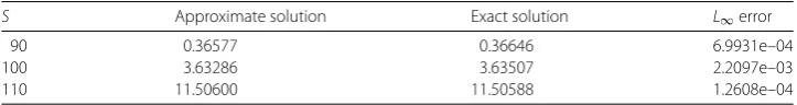
As the ﬁrst numerical example for the European option, we compare the approximate solutions generated by the CCD method and the exact solution under the Merton model without jumps (λ= 0) in Table1with settingM= 128 andN= 25. In Table2, numerical solutions for the European call options obtained by the present method at diﬀerent asset values are presented and compared with the exact solution and the well-known Crank– Nicolson (CN) method. Since the error of the proposed method is of orderO(k2₊_h6_{), in} Table3we set initiallyN= 25 andM= 128 for put options and then increase them by a factor of 8 and 2, respectively.

In Table4, we check the validity of Theorem1by using a numerical example to price European option forλ= 0. In this case, we reduce thehandk so thatΘ=k/h2 _stays constant, and we observe that the stability of the method is established.

Table 1 A comparison between the approximate solution and the exact solution corresponding to the European call options under the Merton model withλ= 0

S Approximate solution Exact solution L_∞error

90 0.36577 0.36646 6.9931e–04

100 3.63286 3.63507 2.2097e–03

110 11.50600 11.50588 1.2608e–04

Table 2 A comparison between the approximate solution and the exact solution corresponding to the European call options under the Merton model withλ= 0.1

K S CN CCD Exact L∞(CN) L∞(CCD)

100 90 0.54524 0.52751 0.52764 1.7602e–02 1.2718e–04

130 32.28254 32.28218 32.28218 3.6643e–04 4.5527e–06

170 71.96107 71.96065 71.96065 4.1983e–04 2.3599e–06

Table 3 Order of convergence for the European put options under the Merton model by the CCD method withλ= 0.1 andS= 30

(M,N) (128, 25) (256, 200) (512, 1600) (1024, 12800)

E=L∞error 1.1753e-04 3.4297e–06 5.9131e–08 9.2704e–10

R=_E₍₂E(M_M,_,8N_N)₎ – 34.2681 58.0014 63.7844

Order= log2R – 5.0988 5.8580 5.9941

Table 4 Check the validity of Theorem1for the European call options under the Merton model: λ= 0,T= 1 andS= 30

(h,k) E=L_∞error

(0.15, 0.1) 8.5571e–05

(0.075, 0.025) 3.0810e–06

(0.0375, 0.0063) 2.4753e–07

(9)

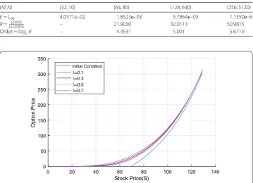
Figure 1European call option prices versus stock prices. Exact and numerical solutions of European call options forS∈[60, 130] andλ= 0.1 (up) and the distribution of absolute error (down)

The curves of the numerical and exact solutions and the distribution of absolute error are plotted in Fig.1, which indicates that our numerical solutions are in good agreement with the exact solution.

5.2 American options

In this section, we perform several numerical simulations to evaluate the prices of Amer-ican options under the Merton model. We used the CCD method, which leads to linear systems involving tridiagonal matrices. It is important to create a highly accurate test so-lution, because there is no analytical solution for the value of an American option. The “exact” option value was computed using the data in [16]. We price an American put op-tion with the following parameters:

σ= 0.15, T= 0.25, r= 0.05,

(10)

Table 5 Values of American put options obtained by the CCD method under the Merton model. The reference values are 10.003822 atS= 90, 3.241251 atS= 100, and 1.419803 atS= 110 [16]. The truncated domain is [–1.5, 1.5] andλ= 0.1,M= 128, andN= 25

S Method [17] CCD method European put L_∞([17]) L_∞(CCD)

90 10.000196 10.0038730 9.28542 3.6e–03 5.1e–05

100 3.231112 3.241153 3.14903 1.1e–02 9.8e–05

110 1.417464 1.419681 1.40119 2.3e–03 1.2e–04

Table 6 Order of convergence of the CCD method for American put options under the Merton model withλ= 0.1

(M,N) (32, 10) (64, 80) (128, 640) (256, 5120)

E=L∞ 4.0571e–02 1.8523e–03 5.7864e–05 1.1350e–6

R=_E₍₂E(M_M,_,8N_N)₎ – 21.9030 32.0113 50.9815

Order = log2R – 4.4531 5.001 5.6719

Figure 2American call option prices versus stock prices. Initial condition and numerical solution under the Merton jump-diﬀusion model for American call options at various states of economy

which are also used by Kwon and Lee [17]. In [17], an implicit method with three-time levels has been used. In Table5, we present the numerical results obtained by using the CCD algorithm. The reference values evaluated by d’Halluin, Forsyth, and Vetzal [16] are with six digits after the decimal point.

To show that the method has sixth-order convergence, we initially setM= 32 andN= 10 for put options, then increase them by a factor of 2 and 8, respectively, in Table6. We use the reference value 10.003822 atS= 90 [16].

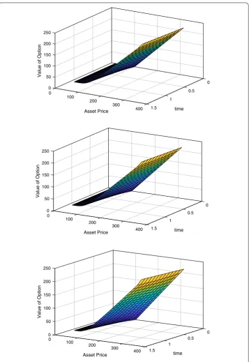
In Fig.2, the initial conditions for American call option are plotted at various states of economy, i.e.,λ= 0.1, 0.3, 0.5, 0.7. In Fig.3, the price of American put option is plotted as a function of time and stock prices.

6 Conclusions

(11)

Figure 3American call option prices versus asset prices. Price of option at various states of economy as a function of stock price and time for American call options under the Merton jump-diﬀusion model. (up) First state of economy (λ= 0.3). (center) Second state of economy (λ= 0.5). (down) Third state of economy (λ= 0.7) withM= 50,N= 10, andS= 70

(12)

Acknowledgements

Authors would like to appreciate the handling editor and the referees for his supports and their useful comments, respectively.

Funding Not applicable.

Availability of data and materials Not applicable.

Competing interests

Authors confirm that SpringerOpen’s guidance on competing interests has been read and there are not any financial and non-financial competing interests for them.

Authors’ contributions

All authors contributed signiﬁcantly to this manuscript, and they read and approved the ﬁnal manuscript.

Authors’ information

Rahman Akbari is currently a PhD student of Financial Mathematics, Reza Mokhtari is currently an Associate Professor of Numerical Analysis, and Mohammad Taghi Jahandideh is currently an Assistant Professor of Mathematical Analysis at the Department of Mathematical Sciences, Isfahan University of Technology, Isfahan 84156-83111, Iran.

Publisher’s Note

Springer Nature remains neutral with regard to jurisdictional claims in published maps and institutional aﬃliations.

Received: 2 May 2019 Accepted: 25 November 2019

References

1. Golbabai, A., Nikan, O.: A computational method based on the moving least-squares approach for pricing double Barrier options in a time-fractional Black–Scholes model. Comput. Econ. (2019).

https://doi.org/10.1007/s10614-019-09880-4

2. Kwork, Y.K.: Mathematical Models of Financial Derivatives, 2nd edn. Springer, Berlin (2011)

3. Rodrigo, M.R., Goard, J.: Pricing of general European options on discrete dividend-paying assets with jump-diﬀusion dynamics. Appl. Math. Model.64, 47–54 (2018)

4. Zhang, H., Liu, F., Turner, I., Chen, S.: The numerical simulation of the tempered fractional Black–Scholes equation for European double barrier option. Appl. Math. Model.40(11–12), 5819–5834 (2016)

5. Amin, K.I.: Jump diﬀusion option valuation in discrete time. J. Finance48, 1833–1863 (1993)

6. Eraker, B., Johannes, M., Polson, N.: The impact of jumps in volatility and returns. J. Finance58, 1269–1300 (2003) 7. Merton, R.C.: Option pricing when the underlying stocks are discontinuous. J. Financ. Econ.5, 125–144 (1976) 8. Cortos, J.C., Sala, R., Jodar, L., Sevilla-Peris, R.: A new direct method for solving the Black–Scholes equation. Appl. Math.

Lett.18, 29–32 (2005)

9. Jodar, L., Company, R., Gonzalez, A.L.: Numerical solution of modiﬁed Black–Scholes equation pricing stock options with discrete dividend. Math. Comput. Model.44, 1058–1068 (2006)

10. Seydel, R.: Tools for Computational Finance. Springer, Berlin (2004)

11. Tavella, D., Randall, C.: Pricing Financial Instruments: The Finite Difference Method. Wiley, New York (2000) 12. Wang, S.: A novel fitted finite volume method for the Black–Scholes equation governing option pricing. IMA J.

Numer. Anal.24, 699–720 (2004)

13. Akbari, R., Mokhtari, R.: A new compact ﬁnite diﬀerence method for solving the generalized long wave equation. Numer. Funct. Anal. Optim.35, 133–152 (2014)

14. Mitchell, A.R., Griffiths, D.F.: The Finite Difference Method in Partial Differential Equations. Wiley, New York (1990) 15. d’Halluin, Y., Forsyth, P.A., Labahn, G.: A penalty method for American options with jump-diffusion processes. Numer.

Math.97, 321–352 (2004)

16. d’Halluin, Y., Forsyth, P.A., Vetzal, K.R.: Robust numerical methods for contingent claims under jump-diﬀusion processes. IMA J. Numer. Anal.25(1), 87–112 (2005)

17. Kwon, Y., Lee, Y.: A second-order tridiagonal method for American options under jump-diﬀusion models. SIAM J. Sci. Comput.33(4), 1860–1872 (2011)

18. Cen, Z., Chen, W.: A HODIE finite difference scheme for pricing American options. Adv. Differ. Equ.2019, 67 (2019). https://doi.org/10.1186/s13662-018-1917-z

19. Rao, S.C.S., Manisha: Numerical solution of generalized Black–Scholes model. Appl. Math. Comput.321, 401–421 (2018)

20. Haq, S., Hussain, M.: Selection of shape parameter in radial basis functions for solution of time-fractional Black–Scholes models. Appl. Math. Comput.335, 248–263 (2018)

21. Safaei, M., Neisy, A., Nematollahi, N.: New splitting scheme for pricing American options under the Heston model. Comput. Econ.52(2), 405–420 (2018)

22. Yang, X., Wu, L., Shi, Y.: A new kind of parallel finite difference method for the quanto option pricing model. Adv. Differ. Equ.2015, 311 (2015).https://doi.org/10.1186/s13662-015-0643-z

23. Zhang, H., Liu, F., Chen, S., Anh, V., Chen, J.: Fast numerical simulation of a new time-space fractional option pricing model governing European call option. Appl. Math. Comput.339, 186–198 (2018)

(13)

26. Chu, P., Fan, C.: A three-point sixth-order nonuniform combined compact diﬀerence scheme. J. Comput. Phys.148, 663–764 (1999)

27. Chu, P., Fan, C.: A three-point sixth-order staggered combined compact diﬀerence scheme. Math. Comput. Model.

32, 323–340 (2000)