Hadronic light-by-light scattering contribution to the muon
g
−
2
on the lattice
NilsAsmussen1,AntoineGérardin2,JeremyGreen3,OleksiiGryniuk1,Georgvon Hippel1,Harvey B.Meyer1,2,
AndreasNyffeler1,∗,VladimirPascalutsa1, andHartmutWittig1,2
1PRISMA Cluster of Excellence and Institut für Kernphysik, Johannes Gutenberg-Universität Mainz, D-55099 Mainz, Germany 2Helmholtz Institut Mainz, D-55099 Mainz, Germany
3John von Neumann Institute for Computing (NIC), DESY, Platanenallee 6, D-15738 Zeuthen, Germany
Abstract.We briefly review several activities at Mainz related to hadronic light-by-light scattering (HLbL) using lattice QCD. First we present a position-space approach to the HLbL contribution in the muong−2, where we focus on exploratory studies of the pion-pole contribution in a simple model and the lepton loop in QED in the continuum and in infinite volume. The second part describes a lattice calculation of the double-virtual pion transition form factorFπ0γ∗γ∗(q21,q22) in the spacelike region with photon virtualities up to 1.5 GeV2which paves
the way for a lattice calculation of the pion-pole contribution to HLbL. The third topic involves HLbL forward scattering amplitudes calculated in lattice QCD which can be described, using dispersion relations (HLbL sum rules), byγ∗γ∗→hadrons fusion cross sections and then compared with phenomenological models.
1 Introduction
The anomalous magnetic moment of the muon has served for many years as a precision test of the Standard Model [1–4] and it has also played an important role in many presentations at this meeting. There is a discrep-ancy of 3−4 standard deviations between experiment and theory for some time now. This could be a signal of New Physics [1, 5], but the uncertainties in the theory prediction from hadronic vacuum polarization (HVP) and hadronic light-by-light scattering (HLbL) make it difficult to draw
firm conclusions. In view of upcoming four-fold more pre-cise new experiments at Fermilab and J-PARC [6], these hadronic contributions need to be better controlled.
The improvement for HVP looks straightforward, with more precise experimental data from various experiments on hadronic cross-sections as input for a dispersion rela-tion [7]. But also lattice QCD is getting more and more precise [8], and, hopefully, also a new method using muon-electron scattering to measure the running of α and the HVP in the spacelike region [9], will be feasible at some point with the required precision.
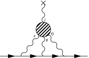
On the other hand, the HLbL contribution to the muon g−2, see Fig. 1, has only been calculated using models so far [1, 4, 10] and the frequently used estimates from Refs. [1, 11, 12] (revised slightly in Ref. [2]) suffer from
uncontrollable uncertainties. In view of this, dispersion re-lations have been proposed a few years ago [13–15] (see also the very recent new proposal in Ref. [16]) to de-termine the presumably numerically dominant contribu-tions from a single neutral pion-pole (light pseudoscalar-pole) and from the two-pion intermediate state (pion-loop) based on input from experimental data for the dispersion
∗Speaker, e-mail: nyff[email protected]
relations. Still some modelling will be needed to estimate the contributions from multi-pion intermediate states, like the axial-vector contribution.
Finally, lattice QCD was proposed some time ago as a model-independent, first principle approach to the HLbL contribution in the muong−2 and some promising progress has been achieved recently by the RBC-UKQCD collaboration [17].
Independently, also the lattice group at Mainz has stud-ied HLbL in recent years. We used complementary ap-proaches to tackle the full HLbL contribution in the muon g−2 with a new position-space approach [18–20], studied the pion transition form factor (TFF) with two virtual pho-tons on the lattice to evaluate the pion-pole contribution to HLbL [21] and we analyzed HLbL forward scattering am-plitudes that can be compared using dispersion relations (HLbL sum rules) [22] to phenomenological models for photon fusion processes [18, 23, 24]. These three topics will be discussed in the following three sections. For all the details, we refer to the quoted papers.
x y
0
z
2 Position-space approach to HLbL in the
muon
g
−
2
on the lattice
The HLbL scattering contribution to the anomalous mag-netic moment of the muon in Fig. 1 can be split into a per-turbative QED kernel ¯Lthat describes the muon and pho-ton propagators and a non-perturbative QCD four-point functioniΠ(denoted by a blob in the Feynman diagram)
that will be evaluated on the lattice.
The projection on the muon g−2 yields the master formula (in Euclidean space notation) [18, 19]
aHLbL
µ = me6
3
d4yd4xL¯
[ρ,σ];µνλ(x, y)
QED
iΠρ;µνλσ(x, y)
QCD
, (1)
with the spatial moment of the four-point function
iΠρ;µνλσ(x, y)=−
d4z z
ρjµ(x)jν(y)jσ(z)jλ(0). (2)
We evaluate the QED kernel in the continuum and in infinite volume and thereby avoid 1/L2 finite-volume
ef-fects from the massless photons. Since Lorentz covariance is manifest in our approach, the eight-dimensional inte-gral in Eq. (1) can be reduced, after contracting all indices, to a three-dimensional integral over the Lorentz invariants x2, y2andx·y.
The QED kernel ¯L[ρ,σ];µνλ(x, y) can be decomposed
into several tensors ¯
L[ρ,σ];µνλ(x, y)=
A=I,II,III GA
δ[ρσ]µανβλT(
A)
αβδ(x, y). (3)
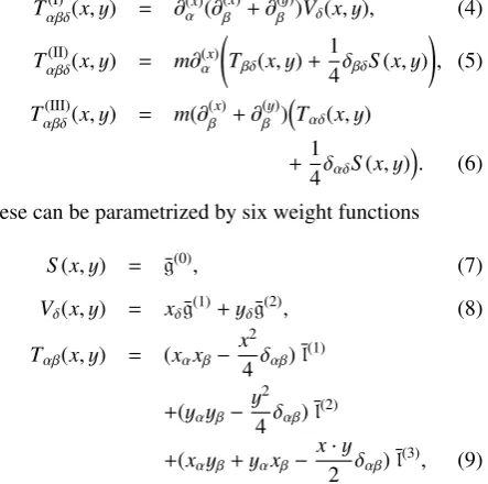
TheGAδ[ρσ]µανβλare traces of gamma matrices and just yield sums of products of Kronecker deltas. The tensorsTαβδ(A)are decomposed into a scalarS, vectorVand tensorT part
Tαβδ(I) (x, y) = ∂α(x)(∂(βx)+∂
(y)
β )Vδ(x, y), (4)
Tαβδ(II)(x, y) = m∂(αx)
Tβδ(x, y)+1
4δβδS(x, y)
, (5)
Tαβδ(III)(x, y) = m(∂β(x)+∂(βy))Tαδ(x, y)
+1
4δαδS(x, y)
. (6)
These can be parametrized by six weight functions
S(x, y) = g¯(0), (7)
Vδ(x, y) = xδg¯(1)+yδ¯g(2), (8)
Tαβ(x, y) = (xαxβ−x
2
4 δαβ) ¯l(1)
+(yαyβ− y2
4δαβ) ¯l(2)
+(xαyβ+yαxβ−x· y
2 δαβ) ¯l(3), (9) that depend on the three variablesx2,x·y=|x||y|cosβand
y2. The semi-analytical expressions for the weight func-tions have been precomputed to about 5 digits precision and stored on a three-dimensional grid. For illustration, the expression for the weight functions ¯g(2)has been given
in Ref. [19]. In Fig. 2 we show the two weight functions ¯
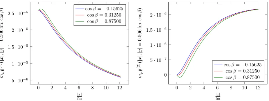
g(1)and ¯g(2)as a function of|x|<12 fm, for a fixed value of|y|=0.506 fm and three values of cosβ. Plots for all six weight functions can be found in Ref. [20].
To test our semi-analytical expressions and the soft-ware for the QED kernel, we have computed theπ0-pole contribution to HLbL in a simple vector-meson domi-nance (VMD) model as well as the lepton-loop contribu-tion toaLbL
µ in QED, where the results are well known. To this aim, we first derived analytical expressions for these contributions to the four-point function iΠρ;µνλσ(x, y) in
position-space, see Ref. [20] for details.
In figure 3 we plot the integrand f(|y|) of the final integration over |y| of the HLbL contribution aHLbL
µ =
∞
0 d|y|f(|y|) (LbL in QED) for these two examples, after
contracting all Lorentz indices and the integrations over|x|
and cosβhave been performed in Eq. (1).
From the plot of the integrand for the pion-pole con-tribution in Fig. 3 one observes that this concon-tribution to aHLbL
µ is remarkably long-range with a long negative tail at large|y|. One expects an exponential decay ∼ e−˜cmπ|y| of the correlation function. But this seems to be coun-tered by some non-negligible power-like behavior|y|n. For
pion masses mπ = 300−900 MeV we reproduce the known results, which can be easily obtained from the three-dimensional integral representation in momentum space given in Ref. [1], at the percent level. On the other hand, for the physical pion mass, one will need rather large lattices of the order of 5−10 fm to capture the negative tail at large|y|in a QCD lattice simulation. Hopefully we can correct for finite-size effects on this contribution, by
com-puting the relevant neutral pion transition form factor on the same lattice ensembles, see Ref. [21] and Section 3.
For the lepton-loop in QED the behavior of the inte-grand for small|y|is compatible with f(|y|)∝ |y|log2(|y|).
This is quite steep and means that we probe the QED ker-nel at small distances. In addition, the height of the pos-itive peak grows with smaller massesmlof the lepton in
the loop. Furthermore there is again a long negative tail at large|y|which demands the use of a large size for the grid where the weight functions have been calculated, in partic-ular for a lepton in the loop that is lighter than the muon. Forml=mµ,2mµwe reproduce the analytically known re-sults foraLbL
µ in QED [25] at the percent level, see Table 1. On the other hand, for the lightest lepton massml=mµ/2, some further refinements of our numerical evaluation are needed. Once this is achieved, we plan to make the QED kernel publicly available.
Table 1.Results (×1011), precision and deviation for the
lepton-loop contribution to LbL in QED with our approach compared to the known results [25]. The first uncertainty originates from the three-dimensional numerical integration, the
second from the extrapolation of the integrand to small|y|.
ml/mµ aLbLµ [25] aLbLµ Prec. Dev.
2 Position-space approach to HLbL in the
muon
g
−
2
on the lattice
The HLbL scattering contribution to the anomalous mag-netic moment of the muon in Fig. 1 can be split into a per-turbative QED kernel ¯Lthat describes the muon and pho-ton propagators and a non-perturbative QCD four-point functioniΠ(denoted by a blob in the Feynman diagram)
that will be evaluated on the lattice.
The projection on the muong−2 yields the master formula (in Euclidean space notation) [18, 19]
aHLbL
µ = me6
3
d4yd4xL¯
[ρ,σ];µνλ(x, y)
QED
iΠρ;µνλσ(x, y)
QCD
, (1)
with the spatial moment of the four-point function
iΠρ;µνλσ(x, y)=−
d4z z
ρjµ(x)jν(y)jσ(z)jλ(0). (2)
We evaluate the QED kernel in the continuum and in infinite volume and thereby avoid 1/L2 finite-volume
ef-fects from the massless photons. Since Lorentz covariance is manifest in our approach, the eight-dimensional inte-gral in Eq. (1) can be reduced, after contracting all indices, to a three-dimensional integral over the Lorentz invariants x2, y2andx·y.
The QED kernel ¯L[ρ,σ];µνλ(x, y) can be decomposed
into several tensors ¯
L[ρ,σ];µνλ(x, y)=
A=I,II,III GA
δ[ρσ]µανβλT(
A)
αβδ(x, y). (3)
TheGAδ[ρσ]µανβλare traces of gamma matrices and just yield sums of products of Kronecker deltas. The tensorsTαβδ(A)are decomposed into a scalarS, vectorVand tensorT part
Tαβδ(I) (x, y) = ∂α(x)(∂(βx)+∂
(y)
β )Vδ(x, y), (4)
Tαβδ(II)(x, y) = m∂(αx)
Tβδ(x, y)+1
4δβδS(x, y)
, (5)
Tαβδ(III)(x, y) = m(∂β(x)+∂(βy))Tαδ(x, y)
+1
4δαδS(x, y)
. (6)
These can be parametrized by six weight functions
S(x, y) = g¯(0), (7)
Vδ(x, y) = xδg¯(1)+yδ¯g(2), (8)
Tαβ(x, y) = (xαxβ−x
2
4 δαβ) ¯l(1)
+(yαyβ− y2
4δαβ) ¯l(2)
+(xαyβ+yαxβ−x· y
2 δαβ) ¯l(3), (9) that depend on the three variablesx2,x·y=|x||y|cosβand
y2. The semi-analytical expressions for the weight func-tions have been precomputed to about 5 digits precision and stored on a three-dimensional grid. For illustration, the expression for the weight functions ¯g(2)has been given
in Ref. [19]. In Fig. 2 we show the two weight functions ¯
g(1)and ¯g(2)as a function of|x|<12 fm, for a fixed value of|y|=0.506 fm and three values of cosβ. Plots for all six weight functions can be found in Ref. [20].
To test our semi-analytical expressions and the soft-ware for the QED kernel, we have computed theπ0-pole contribution to HLbL in a simple vector-meson domi-nance (VMD) model as well as the lepton-loop contribu-tion toaLbL
µ in QED, where the results are well known. To this aim, we first derived analytical expressions for these contributions to the four-point function iΠρ;µνλσ(x, y) in
position-space, see Ref. [20] for details.
In figure 3 we plot the integrand f(|y|) of the final integration over |y| of the HLbL contribution aHLbL
µ =
∞
0 d|y|f(|y|) (LbL in QED) for these two examples, after
contracting all Lorentz indices and the integrations over|x|
and cosβhave been performed in Eq. (1).
From the plot of the integrand for the pion-pole con-tribution in Fig. 3 one observes that this concon-tribution to aHLbL
µ is remarkably long-range with a long negative tail at large|y|. One expects an exponential decay ∼ e−˜cmπ|y| of the correlation function. But this seems to be coun-tered by some non-negligible power-like behavior|y|n. For
pion masses mπ = 300 −900 MeV we reproduce the known results, which can be easily obtained from the three-dimensional integral representation in momentum space given in Ref. [1], at the percent level. On the other hand, for the physical pion mass, one will need rather large lattices of the order of 5−10 fm to capture the negative tail at large|y|in a QCD lattice simulation. Hopefully we can correct for finite-size effects on this contribution, by
com-puting the relevant neutral pion transition form factor on the same lattice ensembles, see Ref. [21] and Section 3.
For the lepton-loop in QED the behavior of the inte-grand for small|y|is compatible with f(|y|)∝ |y|log2(|y|).
This is quite steep and means that we probe the QED ker-nel at small distances. In addition, the height of the pos-itive peak grows with smaller massesml of the lepton in
the loop. Furthermore there is again a long negative tail at large|y|which demands the use of a large size for the grid where the weight functions have been calculated, in partic-ular for a lepton in the loop that is lighter than the muon. Forml=mµ,2mµwe reproduce the analytically known re-sults foraLbL
µ in QED [25] at the percent level, see Table 1. On the other hand, for the lightest lepton massml=mµ/2, some further refinements of our numerical evaluation are needed. Once this is achieved, we plan to make the QED kernel publicly available.
Table 1.Results (×1011), precision and deviation for the
lepton-loop contribution to LbL in QED with our approach compared to the known results [25]. The first uncertainty originates from the three-dimensional numerical integration, the
second from the extrapolation of the integrand to small|y|.
ml/mµ aLbLµ [25] aLbLµ Prec. Dev.
1/2 1229.07 1257.5(6.2)(2.4) 0.5% 2.3% 1 464.97 470.6(2.3)(2.1) 0.7% 1.2% 2 150.31 150.4(0.7)(1.7) 1.2% 0.06%
0 2 4 6 8 10 12
5·10−6 1·10−5 1.5·10−5 2·10−5 2.5·10−5
|x|
fm mµ ¯ g (1) ( | x | , | y | =0 . 506 fm , cos β
) cosβ=−0.15625
cosβ= 0.31250 cosβ= 0.87500
0 2 4 6 8 10 12
0 5·10−7 1·10−6 1.5·10−6 2·10−6
|x|
fm mµ ¯ g (2) ( | x | , | y | =0 . 506 fm , cos β )
cosβ=−0.15625 cosβ= 0.31250 cosβ= 0.87500
Figure 2.The|x|dependence of the weight functions ¯g(1)(left) and ¯g(2)(right) for|y|=0.506 fm and three values of cosβ. Apart from
the scale, the weight functions ¯g(0),¯l(1)and ¯l(2)have the same shape as ¯g(1), whereas ¯l(2)looks similar to ¯g(2).
0 1 2 3 4
0 2 4
|y|/fm
f ( | y | ) × 10 1 0 fm
mπ = 300 MeV
mπ = 600 MeV
mπ = 900 MeV
0 2 4 6 8 10
0 2 4 6 8
|y|/fm
f ( | y | ) × 10 9fm
ml=mµ/2
ml=mµ
ml= 2mµ
Figure 3.(Left) Integrand of the pion-pole contributionaHLbL
µ for a simple VMD transition form factor for three different values of the
pion mass. (Right) Integrand of the lepton-loop contributionaLbL
µ in QED for three different lepton massesmlin the loop.
3 Lattice calculation of the pion transition
form factor
F
π0γ∗γ∗(
q
21,
q
22)
The pion transition form factor can be defined from the following correlation function in Euclidean space, using the methods proposed and used before in Ref. [26]
ME
µν(p,q1) = −
dτeω1τ
d3z e−iq1z
× 0|TJµ(z, τ)Jν(0,0)|π(p)
= µναβq1αq2βFπ0γ∗γ∗(q21,q22), (10)
provided the photon virtualities satisfy q2 1,2 <
min(M2
ρ,4m2π) to avoid poles in the analytical contin-uation from the original definition of the form factor in Minkowski space to Euclidean space. The free real parameter ω1 denotes the zeroth (energy) component of
the four-momentumq1=(ω1, q1).
The main object to compute on the lattice is the three-point function
C(3)
µν(τ,tπ;p, q1, q2) (11)
= a6
x,z
TJν(0,t
f)Jµ(z,ti)P(x,t0) eipxe−iq1z.
Here τ = ti−tf is the time separation between the two
vector currents andtπ = min(tf −t0,ti−t0). The matrix
element in Eq. (10) with an on-shell pion is obtained by considering the limit of largetπ. With the definitions
Aµν(τ) = lim
tπ→+∞ C(3)
µν(τ,tπ)eEπtπ, (12)
Aµν(τ) =
Aµν(τ) τ >0
Aµν(τ)e−Eπτ τ <0 , (13)
one obtains
MEµν = 2Eπ
Zπ
∞
−∞dτe
The overlap factorZπ and the pion energyEπ can be ob-tained from the asymptotic behavior of the pseudoscalar two-point function.
For the calculation of Fπ0γ∗γ∗(q21,q22) on the lattice in Ref. [21] we used eight CLS (Coordinated Lattice Simulations) lattice ensembles [27] with nf = 2
dy-namical quarks with three different lattice spacings a =
(0.048,0.065,0.075) fm and pion masses in the range 194−437 MeV.
We choose the pion rest frame p = 0, with photons
back-to-back spatially q2 = −q1, where the kinematical
range accessible on the lattice is given byq2
1 = ω21−q12,
q2
2 = (mπ −ω1)2−q12. With multiple values of|q1|2 =
2π L
2
|n|2, |n|2 = 1,2,3, . . . we obtain mostly spacelike
photon virtualities up to|q2
1,2| ≈1.5 GeV2, as can be seen
in Fig. 4 (left). In practice, discrete values of ω1 have
been used to sample the momenta. Note that on the lat-tice it is actually easier to access the double-virtual TFF
Fπ0γ∗γ∗(q21,q22), in particular near the diagonalq21=q22, than the single-virtual form factorFπ0γ∗γ∗(q21,2,0) along the two axis, in contrast to the situation in experiments [28].
From the theoretical side, the form factor is con-strained by the chiral anomaly such that Fπ0γ∗γ∗(0,0) = 1/(4π2Fπ) [29] (in the chiral limit). For the single-virtual form factor one expects the Brodsky-Lepage (BL) behav-ior Fπ0γ∗γ∗(−Q2,0) −−−−−→
Q2→∞ 2Fπ/Q
2 [30]. The precise
value of the prefactor is, however, under debate. The double-virtual form factor, where both momenta become simultaneously large, has been computed using the OPE at short distances. In the chiral limit the result reads
Fπ0γ∗γ∗(−Q2,−Q2)−−−−−→
Q2→∞ 2Fπ/(3Q
2) [31].
In order to get a result for the double-virtual TFF
Fπ0γ∗γ∗(q21,q22) in the continuum and for the physical pion mass, we fit our lattice data, obtained for the eight en-sembles with different lattice spacingsaand pion masses
mπ, with three simple models: vector-meson dominance (VMD), lowest-meson dominance (LMD) and LMD+V,
see Refs. [32, 33] for details about these models. The often used VMD model fulfills the BL behavior for the single-virtual case (and describes quite well the available experi-mental data below 2−3 GeV2), but falls offtoo fast for the
double virtual caseFVMD
π0γ∗γ∗(−Q2,−Q2)∼1/Q4. The LMD model is constructed in such a way that it fulfills the OPE constraint, but fails to reproduce the Brodsky-Lepage be-havior. Finally, the LMD+V models is a generalization of
the LMD model and contains two vector resonancesρand ρ. It can be made to fulfill both the BL and the OPE con-straints, for the prize of a large number of free parameters. In order to reduce the number of fit parameters for all the models, a global fit is performed where all lattice en-sembles are fitted simultaneously assuming a linear depen-dence of each model parameter on the lattice spacingaand on the squared pion massm2
π, see Ref. [21] for all the de-tails and results of the fits.
The fits for the VMD and the LMD model are also used to perform the integration in Eq. (14) up to infinite τ, see Fig. 4 (right). For|τ| < 1.3 fm the lattice data are used. The dependence on these models for largeτis small,
but the behavior for smallτis very different. In fact, both
the lattice data and the LMD model show a cusp atτ =
0, which is related to the OPE in the double-virtual case, whereas the VMD model is smooth atτ = 0, since the
VMD model falls offtoo fast at largeQ2.
The VMD model leads to a poor description of our data, withχ2/d.o.f.=2.9 (uncorrelated fit), especially in the double-virtual case and at large Euclidean momenta, see Fig. 5. The normalizationFπVMD0γ∗γ∗(0,0) is offfrom the value expected from the chiral anomaly and the fitted vec-tor meson mass does not agree with theρ-mass.
On the other hand, both the LMD model and the LMD+V model lead to a quite good fit. The LMD model
has aχ2/d.o.f.= 1.3 (uncorrelated fit) and leads to a de-termination of the chiral anomaly at the 7% level, with a value in agreement with expectations. The fitted vector meson mass is close to the rho-meson mass. Furthermore, the fit result for another parameter that is related to the OPE is compatible with the theoretical expections. De-spite the fact that the LMD model fails to reproduce the BL behavior for the single-virtual form factor, this does not seem to affect the global fit, since there are only few
lattice data points at rather low momenta in the single vir-tual case, see Figs. 4 and 5, i.e. one is not yet sensitive to the asymptotic behavior.
Finally, the LMD+V model has aχ2/d.o.f.=1.4 (un-correlated fit), however, only after the model parameters that are related to the two vector meson masses, the BL behavior and the OPE constraint, have been fixed, oth-erwise no stable fit was obtained. The chiral anomaly is reproduced with 9% accuracy and two other fitted model parameters are close to results obtained in phenomenolog-ical analyses of the TFF [33].
The form factors in the three models, extrapolated to the physical point, are shown in Fig. 6. In the single-virtual case, the LMD+V model is in quite good agreement with
the experimental data from Ref. [28]. The LMD model starts to deviate already atQ2 =1 GeV2. In the
double-virtual case, the LMD and LMD+V models are quite
sim-ilar and already close to their asymptotic behavior at the largest pointQ2∼1.5 GeV2where we have lattice data.
Using the LMD+V model at the physical point from
our fit, the pion-pole contribution to HLbL in the muon g−2 can be obtained from the three-dimensional integral representation from Ref. [1], with the result [21],
aHLbL;π0
µ;LMD+V=(65.0±8.3)×10
−11. (15)
Note that the given error is only statistical. No attempt has been made to estimate the systematical errors from using different fit models. Since the relevant momentum
range in the pion-pole contribution is below 1 GeV [34], i.e. where most of our lattice data points are obtained, the extrapolation to large momenta with the LMD+V or
the LMD model does not have a large effect on the
fi-nal result. The result in Eq. (15) is fully consistent with most model calculations which yield results in the range aHLbL;π0
The overlap factorZπ and the pion energyEπ can be ob-tained from the asymptotic behavior of the pseudoscalar two-point function.
For the calculation of Fπ0γ∗γ∗(q21,q22) on the lattice in Ref. [21] we used eight CLS (Coordinated Lattice Simulations) lattice ensembles [27] with nf = 2
dy-namical quarks with three different lattice spacings a =
(0.048,0.065,0.075) fm and pion masses in the range 194−437 MeV.
We choose the pion rest framep = 0, with photons
back-to-back spatially q2 = −q1, where the kinematical
range accessible on the lattice is given byq2
1 = ω21−q12,
q2
2 = (mπ−ω1)2−q12. With multiple values of|q1|2 =
2π L
2
|n|2, |n|2 = 1,2,3, . . . we obtain mostly spacelike
photon virtualities up to|q2
1,2| ≈1.5 GeV2, as can be seen
in Fig. 4 (left). In practice, discrete values of ω1 have
been used to sample the momenta. Note that on the lat-tice it is actually easier to access the double-virtual TFF
Fπ0γ∗γ∗(q21,q22), in particular near the diagonalq21=q22, than the single-virtual form factorFπ0γ∗γ∗(q21,2,0) along the two axis, in contrast to the situation in experiments [28].
From the theoretical side, the form factor is con-strained by the chiral anomaly such that Fπ0γ∗γ∗(0,0) = 1/(4π2Fπ) [29] (in the chiral limit). For the single-virtual form factor one expects the Brodsky-Lepage (BL) behav-ior Fπ0γ∗γ∗(−Q2,0) −−−−−→
Q2→∞ 2Fπ/Q
2 [30]. The precise
value of the prefactor is, however, under debate. The double-virtual form factor, where both momenta become simultaneously large, has been computed using the OPE at short distances. In the chiral limit the result reads
Fπ0γ∗γ∗(−Q2,−Q2)−−−−−→
Q2→∞ 2Fπ/(3Q
2) [31].
In order to get a result for the double-virtual TFF
Fπ0γ∗γ∗(q21,q22) in the continuum and for the physical pion mass, we fit our lattice data, obtained for the eight en-sembles with different lattice spacingsaand pion masses
mπ, with three simple models: vector-meson dominance (VMD), lowest-meson dominance (LMD) and LMD+V,
see Refs. [32, 33] for details about these models. The often used VMD model fulfills the BL behavior for the single-virtual case (and describes quite well the available experi-mental data below 2−3 GeV2), but falls offtoo fast for the
double virtual caseFVMD
π0γ∗γ∗(−Q2,−Q2)∼1/Q4. The LMD model is constructed in such a way that it fulfills the OPE constraint, but fails to reproduce the Brodsky-Lepage be-havior. Finally, the LMD+V models is a generalization of
the LMD model and contains two vector resonancesρand ρ. It can be made to fulfill both the BL and the OPE con-straints, for the prize of a large number of free parameters. In order to reduce the number of fit parameters for all the models, a global fit is performed where all lattice en-sembles are fitted simultaneously assuming a linear depen-dence of each model parameter on the lattice spacingaand on the squared pion massm2
π, see Ref. [21] for all the de-tails and results of the fits.
The fits for the VMD and the LMD model are also used to perform the integration in Eq. (14) up to infinite τ, see Fig. 4 (right). For|τ| < 1.3 fm the lattice data are used. The dependence on these models for largeτis small,
but the behavior for smallτis very different. In fact, both
the lattice data and the LMD model show a cusp at τ =
0, which is related to the OPE in the double-virtual case, whereas the VMD model is smooth at τ = 0, since the
VMD model falls offtoo fast at largeQ2.
The VMD model leads to a poor description of our data, withχ2/d.o.f.=2.9 (uncorrelated fit), especially in the double-virtual case and at large Euclidean momenta, see Fig. 5. The normalizationFπVMD0γ∗γ∗(0,0) is offfrom the value expected from the chiral anomaly and the fitted vec-tor meson mass does not agree with theρ-mass.
On the other hand, both the LMD model and the LMD+V model lead to a quite good fit. The LMD model
has aχ2/d.o.f.= 1.3 (uncorrelated fit) and leads to a de-termination of the chiral anomaly at the 7% level, with a value in agreement with expectations. The fitted vector meson mass is close to the rho-meson mass. Furthermore, the fit result for another parameter that is related to the OPE is compatible with the theoretical expections. De-spite the fact that the LMD model fails to reproduce the BL behavior for the single-virtual form factor, this does not seem to affect the global fit, since there are only few
lattice data points at rather low momenta in the single vir-tual case, see Figs. 4 and 5, i.e. one is not yet sensitive to the asymptotic behavior.
Finally, the LMD+V model has aχ2/d.o.f.=1.4 (un-correlated fit), however, only after the model parameters that are related to the two vector meson masses, the BL behavior and the OPE constraint, have been fixed, oth-erwise no stable fit was obtained. The chiral anomaly is reproduced with 9% accuracy and two other fitted model parameters are close to results obtained in phenomenolog-ical analyses of the TFF [33].
The form factors in the three models, extrapolated to the physical point, are shown in Fig. 6. In the single-virtual case, the LMD+V model is in quite good agreement with
the experimental data from Ref. [28]. The LMD model starts to deviate already atQ2 =1 GeV2. In the
double-virtual case, the LMD and LMD+V models are quite
sim-ilar and already close to their asymptotic behavior at the largest pointQ2∼1.5 GeV2where we have lattice data.
Using the LMD+V model at the physical point from
our fit, the pion-pole contribution to HLbL in the muon g−2 can be obtained from the three-dimensional integral representation from Ref. [1], with the result [21],
aHLbL;π0
µ;LMD+V=(65.0±8.3)×10
−11. (15)
Note that the given error is only statistical. No attempt has been made to estimate the systematical errors from using different fit models. Since the relevant momentum
range in the pion-pole contribution is below 1 GeV [34], i.e. where most of our lattice data points are obtained, the extrapolation to large momenta with the LMD+V or
the LMD model does not have a large effect on the
fi-nal result. The result in Eq. (15) is fully consistent with most model calculations which yield results in the range aHLbL;π0
µ = (50−80)×10−11, but with rather arbitrary, model-dependent error estimates, see Refs. [1, 10, 34] and references therein. 0 0.05 0.1 0.15 0.2
-20 -15 -10 -5 0 5 10 15 20
τ /a
A
(
τ
)
|
q
1|
2= 2
2π L 2 VMD LMD
Figure 4. (Left) Kinematic reach in the photon virtualities (q2
1,q22) with the pion at rest, for a lattice resolution of 643 ×128 with
a=0.048 fm andmπ=268 MeV. (Right) The functionA(τ) (black points) and the VMD (blue line) and LMD (red line) fits used to
describe the tail of the function at largeτfor another lattice ensemble witha=0.065 fm andmπ=270 MeV.
0 0.02 0.04 0.06 0.08 0.1 0.12 0.14 0.16 0.18
0 0.5 1 1.5 2
[Ge
V]
Q2[GeV2] Q2|Fπγ∗γ∗(−Q2,0)|
VMD 0 0.02 0.04 0.06 0.08 0.1 0.12 0.14 0.16 0.18
0 0.5 1 1.5 2
[Ge
V]
Q2[GeV2] Q2|Fπγ∗γ∗(−Q2,0)|
LMD 0 0.02 0.04 0.06 0.08 0.1 0.12 0.14 0.16 0.18
0 0.5 1 1.5 2
[Ge
V]
Q2[GeV2] Q2|Fπγ∗γ∗(−Q2,0)| LMD+V 0 0.02 0.04 0.06 0.08 0.1 0.12
0 0.5 1 1.5 2
[Ge
V]
Q2[GeV2] Q2|F
πγ∗γ∗(−Q2,−Q2)|
VMD 0 0.02 0.04 0.06 0.08 0.1 0.12
0 0.5 1 1.5 2
[Ge
V]
Q2[GeV2] Q2|F
πγ∗γ∗(−Q2,−Q2)|
LMD 0 0.02 0.04 0.06 0.08 0.1 0.12
0 0.5 1 1.5 2
[Ge
V]
Q2[GeV2] Q2|F
πγ∗γ∗(−Q2,−Q2)|
LMD+V
Figure 5.Comparison of the VMD, LMD and LMD+V fits for a lattice ensemble witha=0.048 fm andmπ=268 MeV. The red line
corresponds to the results from our global fit. Note that the points at differentQ2are correlated.
0 0.05 0.1 0.15 0.2
0 0.5 1 1.5 2
[Ge
V]
Q2[GeV2] Q2|F
πγ∗γ∗(−Q2,0)|
VMD LMD LMD+V CELLO CLEO BL 0 0.02 0.04 0.06 0.08 0.1
0 0.5 1 1.5 2
[Ge
V]
Q2[GeV2] Q2|F
πγ∗γ∗(−Q2,−Q2)|
VMD LMD LMD+V OPE
Figure 6. Extrapolation of the lattice data to the continuum and the physical pion mass for the VMD, LMD and LMD+V models.
(Left) Single-virtual form factor, compared with experimental results [28] and the expectation for the asymptotic behavior according to Brodsky-Lepage [30]. (Right) Double-virtual form factor atQ2
4 HLbL forward scattering amplitudes in
lattice QCD
Using parity and time-reversal invariance of QCD, there are eight independent light-by-light forward scattering am-plitudes describing the process γ∗(λ1,q1)γ∗(λ2,q2) →
γ∗(λ1,q1)γ∗(λ2,q2), whereqiandλ()i =0,±are the
mo-menta and helicities of the virtual photons (i = 1,2). Six amplitudes are even and two are odd functions of the crossing-symmetric variableν=q1·q2. The forward
scat-tering amplitudesMλ
1λ2λ1λ2 can be related via the optical theorem to two-photon fusion amplitudes Mλ1λ2 for the processγ∗(λ1,q1)γ∗(λ2,q2)→X(pX) as follows:
Wλ
1λ2,λ1λ2=ImMλ 1λ2,λ1λ2
= 1
2
dΓX(2π)4δ(q1+q2−pX)
× Mλ1λ2(q1,q2,pX)Mλ∗1λ2(q1,q2,pX).(16) Unitarity and analyticity then allow one to write dis-persion relations in ν at fixed values of the virtualities Q2
i =−q2i. Performing one subtraction to get a faster
con-vergence and to suppress higher resonance states, one ob-tains the following sum rules (omitting all dependence on the virtualities and the helicities):
Meven(ν)=Meven(0)+2ν 2
π
∞
ν0
dν Weven(ν)
ν(ν2−ν2−i),
(17)
Modd(ν)=νModd(0)+2ν
3
π
∞
ν0
dν Wodd(ν)
ν2(ν2−ν2−i), (18) with ν0 = (Q21 + Q22)/2. For later use, we
in-troduce the following notation for the subtracted even
M(q2
1,q22, ν) = M(q21,q22, ν) − M(q21,q22,0) and odd M(q2
1,q22, ν)=M(q21,q22, ν)−νM(q21,q22,0) amplitudes.
As proposed first in Ref. [23] for the forward scatter-ing amplitudeMTTand extended recently to all eight
am-plitudes in Ref. [24], the scattering amam-plitudes on the left-hand sides of Eqs. (17)-(18) can be computed from the cor-relation function of four vector currents on the lattice. On the other hand, the right-hand sides of Eqs. (17)-(18) are related to the two-photon fusion processes using Eq. (16). The latter are described by single-meson TFFs which can be parametrized by simple models, as sketched below. Fit-ting the lattice data then determines the model parameters and the TFFs. This will allow one to calculate the contri-butions from single-meson poles to the HLbL contribution in the muong−2.
The lattice simulations are performed on five CLS lat-tice ensembles [27] with two degenerate light dynamical quarks at two lattice spacingsa = 0.048 fm (one ensem-ble) anda=0.065 fm (four ensembles) and pion masses in the range from 194−437 MeV. For all ensembles the fully connected and for two ensembles also the leading quark-disconnected diagrams contributing to the four-point func-tion are taken into account. For each ensemble, the corre-lation function is computed at up to three values of Q2 1
below 0.8 GeV2and for all values ofQ22 ≤4 GeV2. The
result for a subset of four scattering amplitudes is shown in Fig. 7.
The photon fusion reaction on the right-hand sides of Eqs. (17)-(18) can produce any C-parity-even stateX. The main contribution is expected from the pseudoscalar (0−+), scalar (0++), axial-vector (1++) and tensor (2++) mesons, where we consider in each channel only the lightest state. We are working with two degenerate dynamical quarks and fit our phenomenological model to only the fully-connected diagrams. To compensate for this, we include only the contributions from isovector mesons, multiplied by a factor of 34/9 [10, 24].
There is one TFF for the pseudoscalars, two each for the scalars and axial-vectors and four for the tensor mesons [22]. For the pseudoscalars, we take the TFF from Ref. [21] evaluated on the same lattice ensembles. The other TFFs are parametrized as follows
FX(Q21,Q22)= FX(0,0)
1+Q21/Λ2Xn1+Q22/Λ2Xn
, (19)
where we assume a monopole ansatz (n=1) for the scalars
and a dipole ansatz (n=2) for the axial-vectors and tensor
mesons, parametrized by the mass scale ΛX. We assume
one common mass for the scalar TFFs, one mass for the TFFs of the axial-vectors and four different masses for the
TFFs of the tensor mesons. These six masses will be con-sidered as free fit parameters.
The normalization of the TFFs is given by the two-photon decay width and is taken from experiment where available, e.g. for the scalars Γγγ = πα
2
4 mS
FT
Sγ∗γ∗(0,0)
2
(an appropriately defined effective two-photon width is
employed for the axial-vectors [22]). Since not all nor-malizations have been measured, further input from dis-persive sum rules from Ref. [15] is used. Furthermore, for the pseudoscalars, again the lattice data from Ref. [21] are used.
As an example, the pseudoscalar contribution to the cross-sectionσTTof two transversely polarized photons is
given in the narrow-width approximation by
σTT =8π2δ(s−m2P)
Γγγ mP
2√X m2
P
FPγ∗γ∗(Q21,Q22) FPγ∗γ∗(0,0)
2 , (20)
where X = ν2−Q2
1Q22 is the virtual-photon flux factor.
Similar results can be obtained for the other mesons where we assume a Breit-Wigner shape for the resonances [24].
In Fig. 7 the results for four scattering amplitudes of a combined fit to all eight amplitudes with the phenomeno-logical model described above is shown for one lattice en-semble. For four ensembles, theχ2/d.o.f.is quite good, between 1.13−1.35. The fit for the ensemble with the heaviest pion massmπ =437 MeV is, however, not very satisfactory and that ensemble is left out in the chiral ex-trapolation to the physical pion mass.
The relative contribution of the different mesons to
the individual scattering amplitudes was also studied in Ref. [24]. The pseudoscalar and tensor mesons give the dominant contribution to the amplitudes MTT,M
τ
TT and
MaTT that involve two transverse photons. The
4 HLbL forward scattering amplitudes in
lattice QCD
Using parity and time-reversal invariance of QCD, there are eight independent light-by-light forward scattering am-plitudes describing the process γ∗(λ1,q1)γ∗(λ2,q2) →
γ∗(λ1,q1)γ∗(λ2,q2), whereqiandλ()i =0,±are the
mo-menta and helicities of the virtual photons (i = 1,2). Six amplitudes are even and two are odd functions of the crossing-symmetric variableν=q1·q2. The forward
scat-tering amplitudesMλ
1λ2λ1λ2 can be related via the optical theorem to two-photon fusion amplitudes Mλ1λ2 for the processγ∗(λ1,q1)γ∗(λ2,q2)→X(pX) as follows:
Wλ
1λ2,λ1λ2 =ImMλ 1λ2,λ1λ2
= 1
2
dΓX(2π)4δ(q1+q2−pX)
× Mλ1λ2(q1,q2,pX)Mλ∗1λ2(q1,q2,pX).(16) Unitarity and analyticity then allow one to write dis-persion relations in ν at fixed values of the virtualities Q2
i =−q2i. Performing one subtraction to get a faster
con-vergence and to suppress higher resonance states, one ob-tains the following sum rules (omitting all dependence on the virtualities and the helicities):
Meven(ν)=Meven(0)+2ν 2
π
∞
ν0
dν Weven(ν)
ν(ν2−ν2−i),
(17)
Modd(ν)=νModd(0)+2ν
3
π
∞
ν0
dν Wodd(ν)
ν2(ν2−ν2−i),
(18) with ν0 = (Q21 + Q22)/2. For later use, we
in-troduce the following notation for the subtracted even
M(q2
1,q22, ν) = M(q21,q22, ν) − M(q21,q22,0) and odd M(q2
1,q22, ν)=M(q21,q22, ν)−νM(q21,q22,0) amplitudes.
As proposed first in Ref. [23] for the forward scatter-ing amplitudeMTTand extended recently to all eight
am-plitudes in Ref. [24], the scattering amam-plitudes on the left-hand sides of Eqs. (17)-(18) can be computed from the cor-relation function of four vector currents on the lattice. On the other hand, the right-hand sides of Eqs. (17)-(18) are related to the two-photon fusion processes using Eq. (16). The latter are described by single-meson TFFs which can be parametrized by simple models, as sketched below. Fit-ting the lattice data then determines the model parameters and the TFFs. This will allow one to calculate the contri-butions from single-meson poles to the HLbL contribution in the muong−2.
The lattice simulations are performed on five CLS lat-tice ensembles [27] with two degenerate light dynamical quarks at two lattice spacingsa = 0.048 fm (one ensem-ble) anda=0.065 fm (four ensembles) and pion masses in the range from 194−437 MeV. For all ensembles the fully connected and for two ensembles also the leading quark-disconnected diagrams contributing to the four-point func-tion are taken into account. For each ensemble, the corre-lation function is computed at up to three values of Q2 1
below 0.8 GeV2 and for all values ofQ22 ≤4 GeV2. The
result for a subset of four scattering amplitudes is shown in Fig. 7.
The photon fusion reaction on the right-hand sides of Eqs. (17)-(18) can produce any C-parity-even stateX. The main contribution is expected from the pseudoscalar (0−+), scalar (0++), axial-vector (1++) and tensor (2++) mesons, where we consider in each channel only the lightest state. We are working with two degenerate dynamical quarks and fit our phenomenological model to only the fully-connected diagrams. To compensate for this, we include only the contributions from isovector mesons, multiplied by a factor of 34/9 [10, 24].
There is one TFF for the pseudoscalars, two each for the scalars and axial-vectors and four for the tensor mesons [22]. For the pseudoscalars, we take the TFF from Ref. [21] evaluated on the same lattice ensembles. The other TFFs are parametrized as follows
FX(Q21,Q22)= FX(0,0)
1+Q21/Λ2Xn1+Q22/Λ2Xn
, (19)
where we assume a monopole ansatz (n=1) for the scalars
and a dipole ansatz (n=2) for the axial-vectors and tensor
mesons, parametrized by the mass scale ΛX. We assume
one common mass for the scalar TFFs, one mass for the TFFs of the axial-vectors and four different masses for the
TFFs of the tensor mesons. These six masses will be con-sidered as free fit parameters.
The normalization of the TFFs is given by the two-photon decay width and is taken from experiment where available, e.g. for the scalars Γγγ = πα
2
4 mS
FT
Sγ∗γ∗(0,0)
2
(an appropriately defined effective two-photon width is
employed for the axial-vectors [22]). Since not all nor-malizations have been measured, further input from dis-persive sum rules from Ref. [15] is used. Furthermore, for the pseudoscalars, again the lattice data from Ref. [21] are used.
As an example, the pseudoscalar contribution to the cross-sectionσTTof two transversely polarized photons is
given in the narrow-width approximation by
σTT =8π2δ(s−m2P)
Γγγ mP
2√X m2
P
FPγ∗γ∗(Q21,Q22) FPγ∗γ∗(0,0)
2 , (20)
where X = ν2−Q2
1Q22 is the virtual-photon flux factor.
Similar results can be obtained for the other mesons where we assume a Breit-Wigner shape for the resonances [24].
In Fig. 7 the results for four scattering amplitudes of a combined fit to all eight amplitudes with the phenomeno-logical model described above is shown for one lattice en-semble. For four ensembles, theχ2/d.o.f.is quite good, between 1.13−1.35. The fit for the ensemble with the heaviest pion massmπ = 437 MeV is, however, not very satisfactory and that ensemble is left out in the chiral ex-trapolation to the physical pion mass.
The relative contribution of the different mesons to
the individual scattering amplitudes was also studied in Ref. [24]. The pseudoscalar and tensor mesons give the dominant contribution to the amplitudes MTT,M
τ
TT and
MaTT that involve two transverse photons. The
pseu-doscalar meson does not contribute to MT L,MLT where
0 20 40 60 80 100
0 0.5 1 1.5 2 2.5 3 3.5 4
M
TT
Q2 2[GeV2]
Q2
1= 0.352 GeV2
ν[GeV2]
0.117 0.234 0.351 0.467 0.583 0.698 0.812 0.927 1.039
1.150 0
10 20 30 40 50
0 0.5 1 1.5 2 2.5 3 3.5 4
M
a TT
Q2 2[GeV2]
Q2
1= 0.352 GeV2
ν[GeV2]
0.234 0.351 0.467 0.583 0.698 0.812 0.927 1.039 1.150
−70 −60 −50 −40 −30 −20 −10 0 10
0 0.5 1 1.5 2 2.5 3 3.5 4
M
τ TT
Q2 2[GeV2]
Q2
1= 0.352 GeV2
ν[GeV2]
0.117 0.234 0.351 0.467 0.583 0.698 0.812 0.927 1.039
1.150 −10
−5 0 5 10 15 20 25
0 0.5 1 1.5 2 2.5 3 3.5 4
M
LT
Q2 2[GeV2]
Q2
1= 0.352 GeV2
ν[GeV2]
0.117 0.234 0.351 0.467 0.583 0.698 0.812 0.927 1.039 1.150
Figure 7.The forward scattering amplitudesMTT,M
a TT,M
τ
TTandMLT (×106) for a lattice ensemble withmπ=314 MeV and lattice
spacinga=0.065 fm as function ofQ2
2for a fixedQ21=0.352 GeV2and different values ofν. The curves with error-bands represent
the result of the fit of the phenomenological model described in the text to all eight scattering amplitudes withχ2/d.o.f.=1.15.
the main contribution are from axial and tensor mesons. In the amplitudesMaT L,M
τ
T L,MLLscalar, axial and
ten-sor mesons contribute significantly. The contribution from γ∗γ∗ → π+π−, evaluated with scalar QED dressed with a
monopole vector form factor, is always small compared to the other channels.
The lattice simulations are performed for ensembles away from the physical quark masses. The pion and ρ -meson masses are set to their lattice values obtained from the exponential decay of the pseudoscalar and vector two-point functions. For other resonances, we assume a con-stant shift in the massesmX =mphysX +(mlatρ −mexpρ ). In Ta-ble 2 we compare the results of the masses in the TFFs, ex-trapolated to the physical pion mass, to experimental and phenomenological determinations [15, 35]. The agree-ment is reasonably good for MS, MT(2),MT(0,L), although
the scalar mass on the lattice is a bit high. There are quite strong tensions forMA,MT(1),MT(0,T). In particular the
latter two tensor masses on the lattice are almost a fac-tor two larger than the phenomenological determinations. See Ref. [24] for a more detailed discussion and potential reasons for the disagreements. Note in particular, that we have not yet performed the continuum limit.
Overall, we get a good description of the lattice data with the lattice determination of the pion TFF [21] and the simple monopole or dipole ansätze from Eq. (19) for the various TFF’s with one resonance in each channel.
Table 2.Chiral extrapolation to the physical pion mass for the
scalar monopole massMS, the axial dipole massMAand the
four tensor dipole masses corresponding to different helicities, compared to experimental or phenomenological determinations. All masses are given in GeV. The ensembles have a finite lattice spacing ofa=0.065 fm and the ensemble with the largest pion
mass has been excluded in the chiral extrapolation.
Lattice Experiment MS 1.04(14) 0.796(54)
MA 1.32(07) 1.040(80)
M(2)T 1.35(24) 1.222(66) M(1)T 1.69(16) 0.916(20) M(0,T)
T 1.96(09) 1.051(36)
M(0,L)
T 0.67(19) 0.877(66)
5 Conclusions
HLbL is close to current model estimatesaHLbL
µ ≈100× 10−11[1, 2, 11, 12].
Since HLbL involves a rank-four tensor with many independent momenta (or space-time points in position space), it is a very complicated object. We therefore think it makes sense to have as many tests and observables as possible on the lattice, not just the final number foraHLbL
µ itself. Therefore the calculation of the pion (light pseu-doscalar) transition form factor and of HLbL forward scat-tering amplitudes, combined with HLbL sum rules, will be a valuable tool to compare different lattice calculations,
once they become available.
We are grateful for the use of CLS lattice ensembles. We acknowledge the use of computing time on the JUGENE and JUQUEEN machines located at Forschungszentrum Jülich, Ger-many. The correlation functions were computed on the clus-ters “Wilson” at the Institute of Nuclear Physics, University of Mainz, “Clover” at the Helmholtz-Institute Mainz and “Mogon” at the University of Mainz, Germany. This work was par-tially supported by the Deutsche Forschungsgemeinschaft (DFG) through the Collaborative Research Center “The Low-Energy Frontier of the Standard Model” (SFB 1044).
References
[1] F. Jegerlehner and A. Nyffeler, Phys. Rept. 477, 1
(2009).
[2] F. Jegerlehner, EPJ Web Conf.118, 01016 (2016); F. Jegerlehner, arXiv:1705.00263 [hep-ph].
[3] S. Laporta, Phys. Lett. B772, 232 (2017); S. Laporta, talk at this meeting.
[4] M. Knecht, talk at this meeting. [5] D. Stöckinger, talk at this meeting.
[6] T. Gorringe, G. Marshall, talks at this meeting. [7] D. Nomura, V. Sauli, F. Ignatov, A. Denig, talks at
this meeting.
[8] M. Marinkovic, C. Lehner, talks at this meeting. [9] L. Trentadue, U. Marconi, P. Mastrolia, F. Piccinini,
talks at this meeting.
[10] J. Bijnens and J. Relefors, JHEP1609, 113 (2016); J. Bijnens, talk at this meeting, arXiv:1712.09787 [hep-ph].
[11] J. Prades, E. de Rafael and A. Vainshtein, Adv. Ser. Direct. High Energy Phys.20, 303 (2009).
[12] A. Nyffeler, Phys. Rev. D79, 073012 (2009).
[13] G. Colangelo et al., JHEP 1409, 091 (2014); G. Colangelo et al., Phys. Lett. B 738, 6 (2014); G. Colangeloet al., JHEP1509, 074 (2015); Phys. Rev. Lett. 118, 232001 (2017); JHEP 1704, 161 (2017); G. Colangelo, talk at this meeting.
[14] V. Pauk and M. Vanderhaeghen, arXiv:1403.7503 [hep-ph]; Phys. Rev. D90, 113012 (2014).
[15] I. Danilkin and M. Vanderhaeghen, Phys. Rev. D95, 014019 (2017).
[16] F. Hagelstein and V. Pascalutsa, arXiv:1710.04571 [hep-ph].
[17] M. Hayakawa, et al., PoS LAT2005, 353 (2006); T. Blum, M. Hayakawa and T. Izubuchi, PoS LAT-TICE2012, 022 (2012); T. Blumet al., Phys. Rev. Lett.114, 012001 (2015); T. Blumet al., Phys. Rev. D 93, 014503 (2016); T. Blum et al., Phys. Rev. Lett.118, 022005 (2017); Phys. Rev. D96, 034515 (2017); C. Lehner, talk at this meeting.
[18] J. Greenet al., PoS LATTICE2015, 109 (2016). [19] N. Asmussenet al., PoS LATTICE2016, 164 (2016). [20] N. Asmussenet al., arXiv:1711.02466 [hep-lat]. [21] A. Gérardin, H. B. Meyer and A. Nyffeler, Phys. Rev.
D94, 074507 (2016).
[22] V. Pascalutsa and M. Vanderhaeghen, Phys. Rev. Lett.105, 201603 (2010); V. Pascalutsa, V. Pauk and M. Vanderhaeghen, Phys. Rev. D85, 116001 (2012). [23] J. Greenet al., Phys. Rev. Lett.115, 222003 (2015). [24] A. Gérardinet al., arXiv:1712.00421 [hep-lat]. [25] S. Laporta and E. Remiddi, Phys. Lett. B 301, 440
(1993); M. Passera, private communication.
[26] X. d. Ji and C. w. Jung, Phys. Rev. Lett. 86, 208 (2001); Phys. Rev. D64(2001) 034506; J. J. Dudek and R. G. Edwards, Phys. Rev. Lett. 97, 172001 (2006); X. Fenget al., Phys. Rev. Lett.109, 182001 (2012).
[27] P. Fritzschet al., Nucl. Phys. B865, 397 (2012). [28] H. J. Behrendet al.[CELLO Collaboration], Z. Phys.
C49, 401 (1991); J. Gronberget al.[CLEO Collab-oration], Phys. Rev. D57, 33 (1998); B. Aubert et al.[BaBar Collaboration], Phys. Rev. D80, 052002 (2009); S. Ueharaet al.[Belle Collaboration], Phys. Rev. D86, 092007 (2012).
[29] S. L. Adler, Phys. Rev.177, 2426 (1969); J. S. Bell and R. Jackiw, Nuovo Cim. A60, 47 (1969). [30] G. P. Lepage and S. J. Brodsky, Phys. Lett. B87, 359
(1979); Phys. Rev. D22, 2157 (1980); S. J. Brodsky and G. P. Lepage, Phys. Rev. D24, 1808 (1981). [31] V. A. Nesterenko and A. V. Radyushkin, Sov. J. Nucl.
Phys.38, 284 (1983); V. A. Novikov et al., Nucl. Phys. B237, 525 (1984).
[32] B. Moussallam, Phys. Rev. D 51, 4939 (1995); M. Knechtet al., Phys. Rev. Lett.83, 5230 (1999). [33] M. Knecht and A. Nyffeler, Eur. Phys. J. C21, 659
(2001); K. Melnikov and A. Vainshtein, Phys. Rev. D70, 113006 (2004).
[34] M. Knecht and A. Nyffeler, Phys. Rev. D65, 073034
(2002); A. Nyffeler, Phys. Rev. D94, 053006 (2016).