Face Detection and Tracking Techniques: A Review

Volume 2, No. 5, Sept-Oct 2011

International Journal of Advanced Research in Computer Science

REVIEW ARTICLE

Available Online at www.ijarcs.info

Face Detection and Tracking Techniques: A Review

Alankrita Aggarwal

Senior Assistant Professor

Department of Computer Science and Engineering Haryana College of Technology and Management

Kaithal, India [email protected]

Nandita Sethi*

M.Tech (CSE)

Department of Computer Science and Engineering Haryana College of Technology and Management

Kaithal, India [email protected]

Abstract: Face Detection and robustly tracking in a video is a difficult yet important challenge to meet. There are various techniques exits in literature for face detection and tracking. Various face detection methods available in literature like, knowledge based detection, template based detection, feature based and appearance based methods. Out of these, appearance based methods are prominently used. In this paper we are putting light on viola and jones method for face detection. Further for tracking various methods like motion based, predictive learning based methods exits in literature. In this paper we are providing light on optical flow based (motion based) technique. Further these techniques can be merged for robust and real time face detection and face tracking method.

Key Words: Face detection, face tracking, optical flow method, Pyramidal lucas kanade algorithm.

I. INTRODUCTION

Human face detection and tracking is an active area of research covering several disciplines such as image processing, pattern recognition and computer vision. The human face poses even more problems than other objects since the human face is a dynamic object that comes in many forms and colors. However, facial detection and tracking provides many benefits. Facial recognition is not possible if the face is not isolated from the background.

Human Computer Interaction could greatly be improved by using emotion, pose, and gesture recognition, all of which require face and facial feature detection and tracking. Facial Features tracking is a fundamental problem in computer vision due to its wide range of applications in psychological facial expression analysis and human computer interfaces. Recent advances in face video processing and compression have made face-to face communication be practical in real world applications. And after decades, robust and realistic real time face tracking still poses a big challenge. The difficulty lies in a number of issues including the real time face feature tracking under a variety of imaging conditions (e.g., skin color, pose change, self-occlusion and multiple non-rigid features deformation).

There are various techniques exits in literature for facial feature detection and tracking. In this paper a face detector based on the Haar-like features [9] is studied. This face detector is fast and robust to any illumination condition. Further, in this paper we are providing light on optical flow based (motion based) technique. One of the famous optical flow algorithm is the Lucas Kanade algorithm. Pyramidal

Lucas Kanade algorithm [8] is the powerful optical flow algorithm used in feature tracking. It tracks starting from highest level of an image pyramid and working down to lower levels. Tracking over image pyramids allows large motions to be caught by local windows. Also Shi and Thomasi algorithm [4] can be used to extract facial feature points.

II. FACE DETECTION

For face detection, Viola & Jones’s face detector based on the Haar-like features [9] can be used. In [9], Paul Viola and Michael Jones, describes a visual object detection framework that is capable of processing images extremely rapidly while achieving high detection rates. There are three key contributions. The first contribution is a new a technique for computing a rich set of image features using the integral image. The second is a learning algorithm, based on AdaBoost, which selects a small number of critical visual features and yields extremely efficient classifiers [5]. The third contribution is a method for combining classifiers in a “cascade” which allows background regions of the image to be quickly discarded while spending more computation on promising object-like regions.

A. Features Selection:

The main purpose of using features rather than the pixels directly is that features can act to encode ad-hoc domain knowledge that is difficult to learn using a finite quantity of training data. Also the feature-based system operates much faster than a pixel-based system (Viola and Jones method), [9]. The simple features used are reminiscent of Haar basis functions which have been used by Papageorgiou et al. [6] Examples of the features used can be seen in Fig. 1. The features consist of a number of rectangles that are equal in size and horizontally or vertically adjacent.

Figure.1: Rectangle features shown relative to the enclosing detection window.

The sum of the pixels which lie within the white rectangles are subtracted from the sum of pixels in the grey rectangles. Two-rectangle features are shown in (A) and (B) of Fig. 1. (C) in Fig. 1 shows a three-rectangle feature, and (D) in Fig. 1 a four-rectangle feature.

a. Integral Image: Rectangular features can be computed very rapidly using an intermediate representation for the image called the integral image [9]. The integral image at location (x, y) contains the sum of the pixels above and to the left of (x, y), inclusive:

where i(x, y) is the original image and ii(x, y) is the integral image. Using the following pair of recurrences:

s(x, y) = s(x,y-1)+ i(x, y) (1) ii(x, y) = ii(x-1,y) +s(x, y) (2) (where s(x, y) is the cumulative row sum, s (x, -1) = 0 and ii (-1, y) = 0 the integral image can be computed in one pass over the original image.

Using the integral image any rectangular sum can be computed in four array references (Fig. 2). Clearly the difference between two rectangular sums can be computed in eight references. Since the two rectangle features defined above involve adjacent rectangular sums they can be computed in six array references, eight in the case of the three-rectangle features, and nine for four-rectangle features.

Figure. 2: Sum of pixel values within “D”.

The above Fig. 2 showing that the sum of the pixels within rectangle D can be computed with four array references. The value of the integral image at location 1 is the sum of the pixels in rectangle A. The value at location 2 is A + B, at location 3 is A + C, and at location 4 is A + B + C + D. The sum within D can be computed as 4 + 1 - (2 + 3).

B. Learning Classification Functions:

Given a feature set and a training set of positive and negative sample images, any number of machine learning approaches could be used to learn a classification function. A variant of AdaBoost is used both to select the features and to train the classifier [5]. In its original form, the AdaBoost learning algorithm is used to boost the classification performance of a simple (sometimes called weak) learning algorithm. Recall that there are over 117,000 rectangle features associated with each image 24×24 sub-window, a

number far larger than the number of pixels. Even though each feature can be computed very efficiently, computing the complete set is prohibitively expensive. The main challenge is to find a very small number of these features that can be combined to form an effective classifier. In support of this goal, the weak learning algorithm is designed to select the single rectangle feature which best separates the positive and negative examples.

C. Cascade of Classifiers:

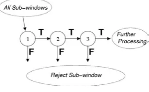
The overall form of the detection process is that of a degenerate decision tree, what we call a “cascade” [2] (see Fig. 3). A positive result from the first classifier triggers the evaluation of a second classifier which has also been adjusted to achieve very high detection rates. A positive result from the second classifier triggers a third classifier, and so on. A negative outcome at any point leads to the immediate rejection of the sub-window.

Figure. 3: Schematic depiction of a the detection cascade.

A series of classifiers are applied to every sub-window. The initial classifier eliminates a large number of negative examples with very little processing. Subsequent layers eliminate additional negatives but require additional computation. After several stages of processing the numbers of sub-windows have been reduced radically. Further processing can take any form such as additional stages of the cascade or an alternative detection system.

III. MOTION DETECTION AND TRACKING

In the field of computer vision motion detection has a relevant importance. By using information contained in a stand image, we can obtain a lot of information about what we are observing, but there is no way to automatically infer what is going to happen in the immediate future. On the other hand a sequence of images provide information about movement of depicted objects. There's a plenty of techniques to recognize movement in a sequence, some based on feature and pattern recognition, some other based just on pixels, regardless what they mean for a human being. Examples are Block Matching analysis and Optical Flow estimation methods etc.

A. Motion and Motion Field:

When an object is moving in space in front of a camera there's a corresponding movement on the image surface. Give the point P0 and its projection Pi, by knowing its velocity V0, we can find out the vector Vi representing its movement in the image (Fig. 4). Given a moving rigid body we can build a motion field by computing all the Vi motion vectors. The motion field is a way to map the movement in a 3D space, on a 2D image taken on camera: for this reason, since we loose a dimension, we cannot exactly compute motion field, but just approximate it.

Figure 5: Example of motion flow

B. Optical Flow:

Optical flow is a phenomenon we deal with every day. It is the apparently visual motion of standing objects as we move through the world. When we are moving the entire world around us seems to move in the opposite way: the faster we move, the faster it does. This motion can also tell us how close we are to the different object we see. The closer they are, the faster their movement will appear. There is also a relationship between the magnitude of their motion and the angle between the direction of our movement and their relative position to us: if we are moving toward an object, it will appear to stand still, but it will become larger as we get closer (this phenomena is also called FOE, focus of expansion); rather, if the object we are looking at is beside us, it will appear moving faster. In computer vision there are a lot of optical flow estimation techniques applied in fields as behaviour recognition or video surveillance; though they are "blinder" than pattern recognition based methods, there are fast enough implementations that allow us to build soft real time applications.

IV. OPTICAL FLOW TRACKING

Optical flow is the apparent motion of image brightness. Let I(x,y,t) be the image brightness that changes in time to provide an image sequence. Two main assumptions can be made [12]:

i. Brightness I(x,y, t) smoothly depends on coordinates x, y in greater part of the image.

ii. Brightness of every point of a moving or static object does not change in time.

Let some object in the image, or some point of an object, move and after time dt the object displacement is (dx,dy). Using Taylor series for brightness I (x,y,t), gives the following:

where “…” are higher order terms.

Then, according to assumption 2,

and

Divide by dt and denote Ixu + Iyv + It = 0

The above equation is called optical flow constraint equation where

are components of optical flow field in x and y

coordinates and the derivatives of I are denoted by subscripts.

The optical flow constraint equation can be rewritten as

We have one equation but two variables, that means we need some other constraints. For this reason optical flow sometimes doesn't correspond to the motion field. This is the so called aperture problem and we can understand it better by watching at Fig. 6, since the cylinder is rotating, if we consider just the black bars, it would be impossible to determine whether they're moving horizontally (as they do), or vertically, as detected by optical flow. It is impossible to determine the real movement unless the end of the bars become visible.

Figure 6: An example when optical flow is different from motion field

A. Aperture Problem:

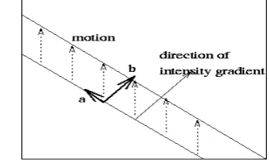
One problem we do have to worry about, however, is that we are only able to measure the component of optical flow that is in the direction of the intensity gradient. We are unable to measure the component tangential to the intensity gradient. This problem is illustrated in Fig. 7, and further developed below.

Figure. 7: The aperture problem. We can only measure the component b.

Since,

Ixu + Iyv + It = 0,

This optical flow constraint equation (which expresses a constraint on the components u and v of the optical flow) can be rewritten as

Thus, the component of the image velocity in the direction of the image intensity gradient at the image of a scene point is

t y

x

u

I

v

I

I

+

=

−

dt dx

u=

dt dy

We cannot, however, determine the component of the optical flow at right angles to this direction. This ambiguity is known as the aperture problem.

B. Optical Flow Methods:

There are different methods that add some constraint to the problem, in order to estimate the optical flow. Some of them are:

a. Block-Based Methods: minimizing sum of squared differences or sum of absolute differences, or maximizing normalized cross-correlation

b. Discrete Optimization Methods: the whole space is quantized, and every pixel is labelled, such that the corresponding deformation minimizes the distance between the source and the target image. The optimal solution is often computed through min-cut max-flow algorithms or linear programming.

c. Differential Methods: The differential methods of optical flow estimation, based on partial spatial and temporal derivatives of the image signal, as following:- d. Lucas-Kanade Method: dividing image into patches and

computing a single optical flow on each of them

e. Horn-Schunck Method: optimizing a functional based on residuals from the brightness constancy constraint, and a particular regularization term expressing the expected smoothness of the flow field.

f. Buxton-Buxton Method: based on a model recovered from the motion of edges in image sequences General variational methods - a range of modifications/extensions of Horn-Schunck, using other data terms and other smoothness terms.

C. Lucas-Kanade Method:

The Lucas-Kanade algorithm [1], as originally proposed in 1981, was an attempt to produce dense results. Yet because the method is easily applied to a subset of the points in the input image, it has become an important sparse technique. The Lucas Kanade algorithm can be applied in a sparse context because it relies only on local information that is derived from some small window surrounding each of the points of interest. The disadvantage of using small local windows in Lucas-Kanade is that large motions can move points outside of the local window and thus become impossible for the algorithm to find. This problem led to development of the “pyramidal” Lucas Kanade algorithm [8], which tracks starting from highest level of an image pyramid (lowest detail) and working down to lower levels (finer detail). Tracking over image pyramids allows large motions to be caught by local windows.

The basic idea of Lucas-Kanade algorithm rests on three assumptions.

a. Brightness constancy: A pixel of an object in an image does not change in appearance as it (possibly) moves from frame to frame. For grayscale image, this means we assume that the brightness of a pixel does not change as is tracked from frame to frame.

b. Temporal Persistence or Small Movements: The image motion of a surface patch changes slowly in time. In practice, this means the temporal increments are fast enough relative to the scale of motion in the image that the object does not move much from frame to frame.

c. Spatial Coherence: Neighboring points in a scene belong to the same surface, have similar motion, and project to nearby points on the image plane.

D. Pyramidal Lucas-Kanade Feature Tracker:

Pyramidal Lucas Kanade algorithm is the powerful optical flow algorithm used in feature tracking. It is a fast algorithm and provides sufficient accuracy and robustness. Consider an image point u = (ux, uy) on the first image I, the goal of feature tracking is to find the location v = u + d in next image J such as I(u) and J(v) are “similar". Displacement vector d is the image velocity at x which also known as optical flow at x [8]. Because of the aperture problem, it is essential to define the notion of similarity in a 2D neighborhood sense. Let ωx and ωy are two integers. then d the vector that minimizes the residual function defined as follows:

Observe that following that definition, the similarity function is measured on a image neighborhood of size (2ωx + 1) x (2ωy +1). This neighborhood will be also called integration window. Typical values for ωx and ωy are 2,3,4,5,6,7 pixels.

i. Functional and Performance Requirements: The

pyramidal algorithm is designed to meet two important requirements for a practical feature tracker:

a. The algorithm should be accurate: The object of a tracking algorithm is to find the displacement of a feature in two different images. An inaccurate algorithm would defeat the purpose of the algorithm in the first place.

b. The algorithm should be robust: It should be insensitive to variables that are likely to change in real world situations. Variables such as variation in lighting, the speed of image motion and patches of the image moving at different velocities. In addition to these requirements, in practice, the algorithm should meet a performance requirement:

c. The algorithm should be computationally inexpensive: The purpose of tracking is to identify the motion of features from frame to frame so the algorithm generally will run at a frequency equal to the frame rate. Most vision systems perform a series of processing functions to meet specific goals and functions that are run at a frequency equal to the frame rate of the source video need to use a little of the system resources as possible.

V. FACIAL FEATURE EXTRACTION

VI. CONCLUSION

To detect the face in the image, a face detector based on the Haar-like features can be used. This face detector is fast and robust to any illumination condition. For facial feature point extraction, Shi and Tomasi Method can be used. In this paper we are providing light on optical flow based (motion based) technique. In order to track the facial feature points, Pyramidal Lucas-Kanade Feature Tracker algorithm can be used. Pyramidal Lucas Kanade algorithm is the powerful optical flow algorithm used in feature tracking. Further these techniques can be merged for robust and real time face detection and face tracking method.

VII. REFERENCES

[i]. B. D. Lucas and T. Kanade, “An iterative image registration technique with an application to stereo vision,” Proceedings of the DARPA Imaging Understanding Workshop, pp. 121–130, 1981.

[ii]. J. Quinlan, “Induction of decision trees,” Machine Learning, Journal, vol. 1, no. 1, pp. 81-106, 1986.

[iii]. M. Lades, J.C. Vorbrüggen, J. Buhmann , J. Lange, C. Malsburg, R. Würtz., and W. Konen, “Distortion invariant object recognition in the dynamic link architecture,” IEEE Trans. Computer, vol. 42, no. 3, pp. 300-310, 1993.

[iv]. J. Shi and C. Tomasi, “Good Features to Track,” IEEE Conference on Computer Vision and Pattern Recognition, pp. 593-600, 1994.

[v]. Y. Freund and R.E. Schapire, “A decision-theoretic generalization of on-line learning and an application to boosting,” in European Conference on Computational Learning Theory, pp. 23–37, 1995.

[vi]. C. Papageorgiou, M. Oren, and T. Poggio, “A general framework for object detection,” In International Conference on Computer Vision, vol. 21, pages 555– 562, 1998.

[vii]. K. Sung and T. Poggio, “Example-based learning for view-based face detection,” IEEE Transactions on

Pattern Analysis and Machine Intelligence, volume 20, pp. 39–51, 1998.

[viii]. J.Y. Bouguet, “Pyramidal Implementation of the Lucas Kanade Feature Tracker Description of the algorithm,” Intel Corporation, Microprocessor Research Labs, pp. 1-9, 2000.

[ix]. P. Viola and M. Jones, “Robust Real-time Object Detection,” 2nd international workshop on statistical and computational theories of vision - modeling, learning, computing, and sampling, pp. 1-25, 2001.

[x]. E. Hjelmas and B.K. Low, “Face detection: a survey,” Computer vision and image understanding, vol. 83, pp. 236-274, 2001.

[xi]. M. H Yang, “Detecting faces images, A survey,” IEEE Transations on Pattern Analysis and Machine Inteligence vol. 24, no. 1, pp. 34–58, 2002.

[xii]. Z. Vamossy, A. Toth, and P. Hirschberg, ”PAL Based Localization Using Pyramidal Lucas-Kanade Feature Tracker”, In 2nd Serbian-Hungarian Joint Symposium on Intelligent Systems, Subotica, Serbia and Montenegro, pp. 223-231, 2004.

[xiii]. K.S. Huang, and M.T. Trivedi , “Robust real-time detection, tracking, and pose estimation of faces in video streams,” Proceedings of the 17th International Conference on Pattern Recognition, Vol. 3 pp. 965 - 968 , 2004.

[xiv]. L. Stan and Z. Zhang, “FloatBoost learning and statistical face detection”, IEEE Trans. On Pattern Analysis and Machine Intelligence. vol. 26, no. 9, pp. 1112-1123, 2004.

[xv]. P. Menezes, J. C. Barreto, and J. Dias, “face tracking based on haar like features and eigen faces,” 5th IFAC Symposium on Intelligent Autonomous Vehicles, Lisbon, Portugal, pp. 1-6, July 5-7, 2004.