Bayesian approach with prior models which enforce sparsity in signal and image processing

R E V I E W

Open Access

Bayesian approach with prior models which

enforce sparsity in signal and image processing

Ali Mohammad-Djafari

Abstract

In this review article, we propose to use the Bayesian inference approach for inverse problems in signal and image processing, where we want to infer on sparse signals or images. The sparsity may be directly on the original space or in a transformed space. Here, we consider it directly on the original space (impulsive signals). To enforce the sparsity, we consider the probabilistic models and try to give an exhaustive list of such prior models and try to classify them. These models are either heavy tailed (generalized Gaussian, symmetric Weibull, Student-t or Cauchy, elastic net, generalized hyperbolic and Dirichlet) or mixture models (mixture of Gaussians, Bernoulli-Gaussian, Bernoulli-Gamma, mixture of translated Gaussians, mixture of multinomial, etc.). Depending on the prior model selected, the Bayesian computations (optimization for the joint maximum a posteriori (MAP) estimate or MCMC or variational Bayes approximations (VBA) for posterior means (PM) or complete density estimation) may become more complex. We propose these models, discuss on different possible Bayesian estimators, drive the

corresponding appropriate algorithms, and discuss on their corresponding relative complexities and performances.

Keywords:sparsity, Bayesian approach, sparse priors, inverse problems

1 Introduction

In many generic inverse problems in signal and image processing we want to infer on an unknown signal f(t) or an unknown image f(r) with r = (x, y) through an observed signalg(s) or an observed image g(s) related between them through an operator_Hsuch as convolu-tiong=h* for any other linear or non linear transfor-mation g=Hf. When this relation is linear and we have discretized the problem, we arrive to the relation:

g=Hf +ε, (1) wheref = [f1, ...,fn]’represents the unknowns,g= [g1, ...,gm]’ the observed data,= [1, ...,m]’ the errors of

modeling and measurement and H the matrix of the system response. We may note that, even if the noise could be neglected (= 0) and the matrixH invertible (m=n), in general, the solutionf =H−1g is not forcibly the good solution, because this solution may be too sen-sitive to small changes in the data due to the ill-condi-tioning of this matrix. for the general case ofm≠n, one tries to obtain a regularized solution, for example by

defining it as the optimizer of a two parts criterion

_{f = arg min}

f {J(f) =

g−Hf2+λf2} (2)

which is given by_{f = [HH+λI]}−1_Hg. When the reg-ularization parameter l = 0, one gets a generalized inverse_{f = [HH]}−1_Hgand whenH invertible, one gets the normal inverse solutionf =H−1g. The regulariza-tion theory has been developed since the pioneer work of Tikhonov [1] and Tikhonov and Arsénine [2] who had introduced a quadratic regularization terms to account for some prior properties of the solution (smoothness). Since that, many different regularization terms have been proposed. In particular, in place ofL2

norm: L2(f) =f2₂=

jfj 2

, it has been proposed to

use the L0 normL0(f) =f₀=jδ(fj)or the L1 norm

L1(f) = ||f||1 =Σj|fj| to enforce the sparsity of the

solu-tion [3-11]. Then, due to the fact that L0(f) is not con-vex and L1(f) is convex, but not continuous, the optimization of a criterion with these expressions becomes more difficult than theL2 norm case. For this reason, there was a great number of works who

Correspondence: [email protected]

Laboratoire des signaux et systèmes (L2S), UMR 8506 CNRS-SUPELEC-UNIV PARIS SUD, SUPELEC, Plateau de Moulon, 91192 Gif-sur-Yvette, France

specialized in proposing algorithms for the optimization of such criteria.

Interestingly, defining the solution of the problem (1) as the optimization of a criterion with two parts can be assimilated to a maximum a posteriori (MAP) solution in a Bayesian approach where the first term of the cri-terion (2) can be related to the likelihood and the sec-ond term to a prior model as we will see in the following where the main objective is to show how the Bayesian approach can go farther than the regularization in at least the following aspects:

•A better account for the noise term characteristics;

• A better and easier way for translating the prior knowledge and in particular the sparsity;

• New tools for assessing the regularization para-meter, a great subject of discussion for all those work with regularization theory;

• New solutions and new tools for doing computa-tions (optimizacomputa-tions and integracomputa-tions).

1.1 The Bayesian approach

The Bayesian inference approach is based on the poster-ior law:

p(fg,θ1,θ2) =

p(gf,θ1)p(f|θ2) p(g|θ1,θ2) ∝

p(gf,θ1)p(f(3)|θ2) where the sign∝ stands for “proportional to”, p(g|f,

θ1) is the likelihood,p(f|θ2) the prior model,θ= (θ1,θ2) are their corresponding parameters (often called the hyper parameters of the problem) and p(g|θ1, θ2) is called the evidence of the model.

This general Bayesian approach is illustrated as fol-lows:

In this approach, the likelihoodp(g|f, θ1) summarizes our knowledge about the noise and the model linking the observed data gto the unknowns f and the prior term p(f|θ2) summarizes our incomplete prior knowl-edge about the unknowns and the posterior lawp(f|g, θ) combines these two terms and contains all our state of knowledge about the unknowns f after accounting for the prior and the observed data.

As a very simple example, when the noise is assumed

to be Gaussian, then the MAP solution

_{f = arg maxf{p(fg,θ)}}is obtained as the optimizer of the criterionJ(f) = ||g-Hf||2+lΩ(f) where the expres-sion of Ω(f) depends on the prior law. When the prior

knowledge is translated as a Gaussian probability law, then(f) =f2₂and when it is translated as a Laplace probability law, thenΩ(f) = ||f||1 [12-14].

The first interest of using the Bayesian approach to the regularization approach is to have new tools for handling the hyper parameters [15].

1.2 Full Bayesian approach

When the parameters θ have to be estimated too, we can assign them a prior p(θ|θ0) with fixed values for θ0 (often called hyper-hyper-parameters) and express the joint posterior

p(f,θg,θ0) =

p(gf,θ1)p(f|θ2)p(θ|θ0) p(g|θ0)

(4)

and then try to estimate them jointly, for example joint MAP [16]:

(f,θ) = arg max (f,θ){p(f,θ

g,θ0)} (5)

This Full Bayesian approach is illustrated as follows:

One may also first integrate out one of them, for examplefto obtain

p(θg,θ0) =

p(f,θg,θ0) df, (6) estimateθ, for example by

_{θ= arg max}

θ {p(θg,θ0)} (7)

and then use it for the estimation of the other one usingp(fg,θ).

This approach (called sometimes type II maximum likelihood) is illustrated as follows:

incomplete data log-likelihoodand ln p(g, f|θ)complete data log-likelihood, the classical EM algorithm writes:

⎧ ⎨ ⎩

E - step :q(θ,θ(k)) = E p(f|g,θ(k)

){lnp(g,f|θ)} M - step:θ(k)= arg maxθ

q(θ,θ(k−1))

(8)

The Bayesian version (Bayesian EM) is not very far and differs only by the introduction ofp(θ):

⎧ ⎨ ⎩

E - step :q(θ,θ(k)) = E

p(fg,θ(k)){lnp(g,f|θ) + lnp(θ)} M - step :θ(k)= arg maxθ

q(θ,θ(k−1))

(9)

This is illustrated as follows:

As we mentioned before, one of the main steps in the Bayesian approach is the prior modeling which has the role of translating our prior knowledge on the unknown signal or image in a probability law. Sparsity is one of the prior knowledge we may translate. The main objec-tive of this article is to see what are the different possibilities.

1.3 Prior modeling

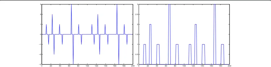
In this article, we propose different prior modeling for signals and images which can be used in a Bayesian inference approach in many inverse problems in signal and image processing where we want to infer on sparse signals or images. The sparsity may be directly on the original space or in a transformed space (see Figures 1, 2, 3, and 4). In this article, we consider the sparsity directly in the original domain.

The prior models discussed are the following:

- generalized Gaussian (GG) with Gaussian (G) and Laplace or double exponential (DE) as particular cases;

- symmetric Weibull (W) with symmetric Rayleigh (R) and again the DE as particular cases;

- Student-t (St) with Cauchy (C) as particular case;

- Elastic net prior model; - generalized hyperbolic model; - Dirichlet and symmetric Dirichlet;

- Mixture of two centered Gaussians (MoG2), one with very small and one with a large variances;

- Bernoulli-Gaussian (BG), also calledSpike and slab; - Mixture of two Gammas (MoGamm);

- Bernoulli-Gamma (BGamma);

- Mixture of three Gaussians (MoG3), one centered with very small variance and two symmetrically centered on positive and negative axes and large variances;

- Mixture of one Gaussian and two Gammas (MoG-Gammas), and in a more summary the case of

- Bernoulli-Multinomial (BMult) or mixture of Dirich-let (MoD).

Some of these models are well-known [12-14,18-26], some others less. In general, we can classify them into two categories: (i) simple non Gaussian models with heavy tails and (ii) mixture models with hidden variables which result to hierarchical models.

In the Section 2, we give more details about the spar-sity and all these prior models which enforce the sparsity.

1.4 Bayesian computation

The second main step in the Bayesian approach is to do the computations. Depending on the prior model selected, the Bayesian computations needed are:

•For simple prior models:

- Simple optimization ofp(f|θ,g) for the MAP:

- Joint optimizationp(f,θ|g) for joint MAP:

0 20 40 60 80 100 120 140 160 180 200

−3

−2

−1 0 1 2 3

0 20 40 60 80 100 120 140 160 180 200 0

0.5 1 1.5 2 2.5 3

- Generation of samples from the conditionalsp (f|θ, g) andp(θ|f, g) for the MCMC Gibbs sam-pling methods,

- Variational approximation (VA) of the jointp(f,

θ|g) by a separable

q(f,θg) =q1(fθ ,g)q2(θf,g) and then using them for estimation

•For hierarchical prior models with hidden variables

z:

- Joint optimizationp(f,z,θ|g) for joint MAP,

- Generation of samples from the conditionalsp (f|z, θ, g), p(θ|z, f, g) and p(z|f, θ, g) for the MCMC Gibbs sampling methods:

0 20 40 60 80 100 120 140 160 180 200

−6

−4

−2 0 2 4 6

0 20 40 60 80 100 120 140 160 180 200

−1

−0.8

−0.6

−0.4

−0.2 0 0.2 0.4 0.6 0.8 1

0 0.1 0.2 0.3 0.4 0.5 0.6 0.7 0.8 0.9 1 0

20 40 60 80 100 120 140 160 180 200

20 40 60 80 100 120 140 160 180 200 1

2

3

4

5

6

7

8

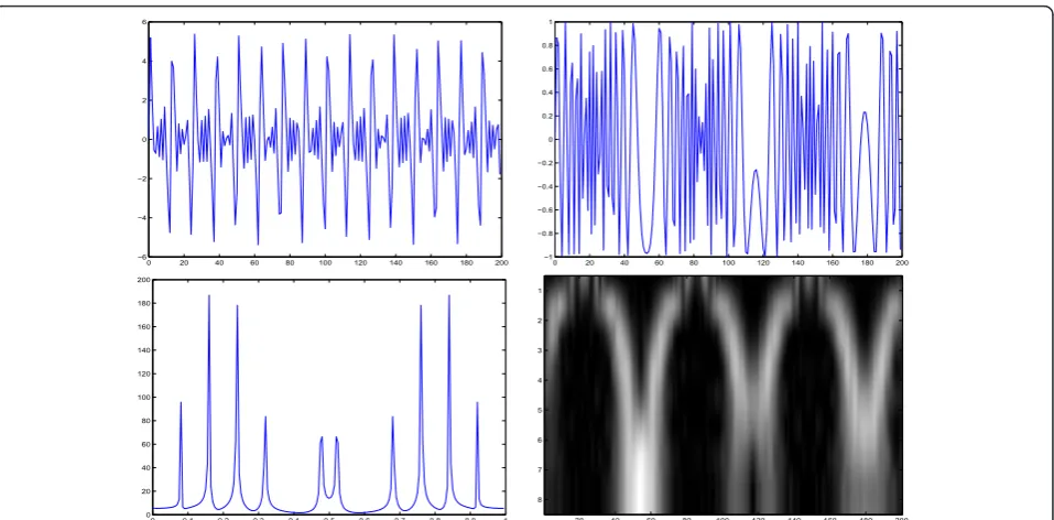
Figure 2Sparsity: sparse signals in a transformed domaine (Fourier or wavelet). First row: signals, second row: Fourier or wavelet transforms.

50 100 150 200 250 50

100

150

200

250

50 100 150 200 250 50

100

150

200

250

- Variational approximation (VA) of the jointp(f,

z,θ|g) by a separable

q(f,z,θg) =q1(fz,θ,g)q2(zf,θ,g)q3(θz,f,g) and then using them for estimation

The second main objective of this article is to discuss on the relative complexities and performances of the algorithms obtained with the proposed prior law.

The rest of the article is organized as follows:

In Section 2, we present in details the proposed prior models and discuss their properties. For example, we will see that the Student-t model can be interpreted as an infinite mixture with a variance hidden variable or that the BG model can be considered as the degenerate case of a MoG2 where one of the variances go to zero. Also, we will examine the less known models of MoG3 and MoGGammas where the heavy tails are obtained by combining a centered Gaussian and two large variance non-centered Gaussians or Gammas.

In Section 3, we examine the expression of the poster-ior laws that we obtain using these prposter-iors and discuss then on complexity of the Bayesian computation of the algorithms. In particular for the mixture models, we give details of the joint estimation of the signal and the

hidden variable as well as the hyper parameters (para-meters of the mixtures and the noise) for unsupervised cases.

In Section 4, we give more details on the variational Bayesian approximation method, first for the general case and then for the case of mixture laws and more specifically the case of the Student-t considered as a continuous mixture.

Finally, we present the main conclusions of this article in Section 5.

2 Prior models enforcing sparsity

First, as we mentioned, the sparsity is a property which can be described either directly for the signal itself or after some transformation, for example on the derivative of the signal, or in more general on the coefficients of the projection of the signal on any basis or any set of functions.

Different prior models have been used to enforce sparsity.

2.1 Generalized Gaussian (GG), Gaussian (G) and double exponentials (DE) models

This is the simplest and the most used model (see for example, [27]). Its expression is:

p(f|γ,β) = j

GG(fj|γ,β)∝exp

⎧ ⎨ ⎩−γ

j

fjβ

⎫ ⎬ ⎭(10)

50 100 150 200 250

50

100

150

200

250

50 100 150 200 250

50

100

150

200

250

50 100 150 200 250

50

100

150

200

250

where

GG(fj|γ,β) = βγ

2(1/β)exp{−γfj

β_}.

(11)

Two particular cases are of importance:

•b= 2 (Gaussian):

p(f|γ) =

j

N(fj0, 1/(2γ) )∝exp

⎧ ⎨ ⎩−γ

j

fj

2 ⎫ ⎬ ⎭

∝exp{−γf2₂}

(12)

•b= 1 (double exponential or Laplace):

p(f|γ) = j

DE(fj|γ)∝exp

⎧ ⎨ ⎩−γ

j

fj

⎫ ⎬ ⎭

∝exp{−γf₁}

(13)

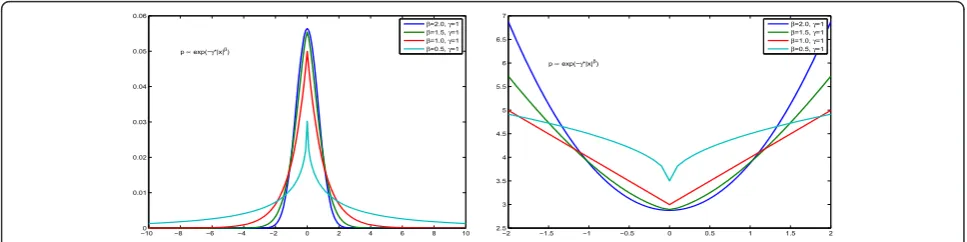
The general shape of these priors are shown in Figure 5, where the cases b = 1 and 0 <b < 1, which are of great interest for sparsity enforcing are compared to the Gaussian caseb= 2.

2.2 Symmetric Weibull (W) and symmetric Rayleigh (R) models

The second model we consider is the symmetric Wei-bull probability density function (pdf):

p(f|γ,β) = j

W(fj|γ,β)

∝exp

⎧ ⎨ ⎩−γ

j

fjβ+ (β−1) logfj

⎫ ⎬ ⎭

(14)

where

W(fj|γ,β) =cfj(β−1)exp{−γfjβ} (15)

and where g> 0 andb> 0, and the particular cases of

b = 1 is the double exponential and b= 2 is the sym-metric Rayleigh distribution:

p(f|γ,β) =

j

R(fj|γ)∝exp

⎧ ⎨ ⎩−γ

j

_fj2

+ logfj

⎫ ⎬ ⎭(16)

the cases where 0 <b< 1 are of great interest for sparsity enforcing. This family of models are illustrated on Figure 6.

−010 −8 −6 −4 −2 0 2 4 6 8 10

0.01 0.02 0.03 0.04 0.05 0.06

p∝ exp(−γ*|x|β)

β=2.0,γ=1

β=1.5,γ=1

β=1.0,γ=1

β=0.5,γ=1

−2 −1.5 −1 −0.5 0 0.5 1 1.5 2

2.5 3 3.5 4 4.5 5 5.5 6 6.5 7

p∝ exp(−γ*|x|β)

β=2.0,γ=1

β=1.5,γ=1

β=1.0,γ=1

β=0.5,γ=1

Figure 5Generalized Gaussian family. The probability density functionp(x) is shown in the left and - lnp(x) is shown in the right.

−010 −8 −6 −4 −2 0 2 4 6 8 10

0.05 0.1 0.15 0.2 0.25 0.3 0.35

p∝ exp(−γ*(|x|β+(β−1)*log(|x|))

β=2.0,γ=1.0

β=1.5,γ=1.0

β=1.0,γ=1.0

β=1.0,γ=0.5

−2 −1.5 −1 −0.5 0 0.5 1 1.5 2

1 2 3 4 5 6 7 8 9

p∝ exp(−γ*(|x|β+(β−1)*log(|x|))

β=2.0,γ=1.0

β=1.5,γ=1.0

β=1.0,γ=1.0

β=1.0,γ=0.5

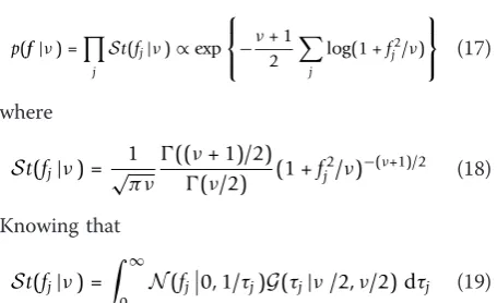
2.3 Student-t (St) and Cauchy (C) models

The second simplest model is the Student-t model:

p(f|ν) = j

St(fj|ν)∝exp

⎧ ⎨ ⎩−ν

+ 1 2

j

log(1 +fj2/ν)

⎫ ⎬

⎭ (17)

where

St(fj|ν) = 1

√_πν((ν + 1)/2) (ν/2) (1 +f

2

j/ν)−(ν+1)/2 (18)

Knowing that

St(fj|ν) =

_∞

0

N(fj0, 1/τj)G(τj|ν/2,ν/2) dτj (19)

we can write this model via the positive hidden vari-ablesτj:

p(f,τ) =jp(fjτj) =

jN(fj0, 1/τj) ∝exp

−1 2

jτjf 2 j

p(τj|a,b) =G(τj|a,b)∝τj(a−1)exp{−bτj} witha=b=ν/2

(20)

Cauchy model is obtained whenν= 1:

p(f) = j

C(fj)∝exp

⎧ ⎨ ⎩−

j

log(1 +f_j2)

⎫ ⎬

⎭ (21)

This family of models are illustrated on Figure 7.

2.4 Elastic Net (EN) prior model

A prior model inspired from elastic net regression litera-ture [28] is:

p(f|ν) =

j

EN(fj|ν)∝exp

⎧ ⎨ ⎩−

j

(γ1fj+γ2fj2)

⎫ ⎬ ⎭ (22)

where

EN(fj|ν) =N(0, 1/γ1)DE(γ1)∝exp

−γ1fj−γ2fj2)

(23)

which is a product of a Gaussian and a double expo-nential pdfs. This family of models are illustrated on Figure 8.

2.5 Generalized hyperbolic (GH) prior model Another general prior model which can be used is:

p(f|δ,ν,β) = j(δ

2_+f2 j)

(ν−1/2)/2

exp{βx}

K_ν−1/2(α

δ2_+f2 j )

(24)

where Kν-1/2 is the second kind Bessel function of order (ν- 1/2). This family of models are illustrated on Figure 9.

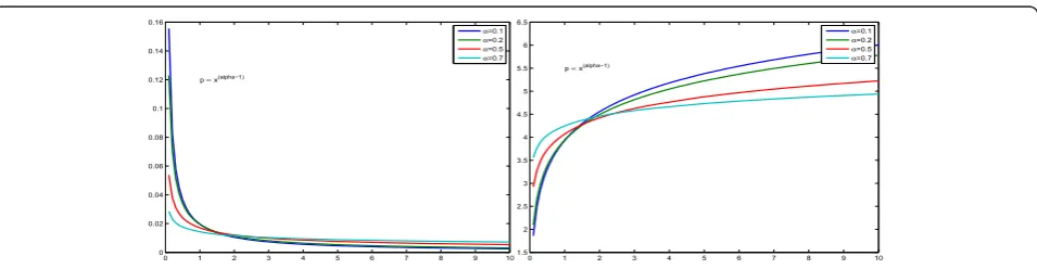
2.6 Dirichlet (D) and symmetric Dirichlet (SD) models When fj are positive and sums to one, we can use the

Dirichlet model

D(f|α)∝ j

fαj−1

j with fj>0,

j

fj= 1 ₍₂₅₎

wherea= {a1, ...,aN} withaj> 0. The proportionality

constant is

B(α) =

j(αj) j(αj)

₍₂₆₎

It is noted that the support of this distribution is [0,1]

N

and ||f||1 =Σjfj= 1.

It is also interesting to note that the domain of the Dirichlet distribution is itself a probability distribution, specifically a N-dimensional discrete distribution and the set of points in the support of a N-dimensional Dirichlet distribution is the open standard N- 1-sim-plex, which is a generalization of a triangle, embedded in the next-higher dimension.

−010 −8 −6 −4 −2 0 2 4 6 8 10

0.02 0.04 0.06 0.08 0.1 0.12 0.14

p∝ exp(−((ν+1)/2)*log(1+|x|2₎₎

ν=1

ν=2

ν=5

ν=10

−2 −1.5 −1 −0.5 0 0.5 1 1.5 2

2 3 4 5 6 7 8 9 10 11

p∝ exp(−((ν+1)/2)*log(1+|x|2₎₎

ν=1

ν=2

ν=5

ν=10

A very common special case is thesymmetric Dirichlet (SD) distribution, where all of the elements making up the parameter vectorahave the same valueacalled the concentration parameter:

D(f|α)∝ j

f_jα−1withfj>0,

j

fj= 1 ₍₂₇₎

When a > 1, the symmetric Dirichlet distribution is equivalent to a uniform distribution over the open stan-dard stanstan-dard N- 1-simplex, i.e., it is uniform over all points in its support. a > 1 prefer variants that are dense, evenly-distributed distributions, i.e., all probabil-itiesfj returned are similar to each other.a < 1 prefer

sparse distributions, i.e., most of the probabilities fj

returned will be close to 0, and the vast majority of the mass will be concentrated in a few of them. This is the case on which we are interested. An illustration of this family of models are illustrated on Figure 10.

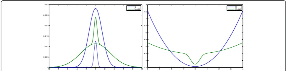
2.7 Mixture of two Gaussians (MoG2) model

The mixture models are also very commonly used as prior models. In particular the mixture of two Gaussians (MoG2) model:

p(f|λ,v1,v0) =

j

(λN(fj|0,v1) + (1−λ)N(fj|0,v0))₍₂₈₎

−010 −8 −6 −4 −2 0 2 4 6 8 10

0.02 0.04 0.06 0.08 0.1 0.12

p∝ exp(−γ1*|x|−γ2*x 2₎

γ1=0.1,γ2=0.1

γ1=0.5,γ2=0.1

γ1=1.0,γ2=0.1

γ1=2.0,γ2=0.1

−2 −1.5 −1 −0.5 0 0.5 1 1.5 2

2 2.5 3 3.5 4 4.5 5 5.5 6 6.5 7

p∝ exp(−γ1*|x|−γ2*x2)

γ1=0.1,γ2=0.1

γ1=0.5,γ2=0.1

γ1=1.0,γ2=0.1

γ1=2.0,γ2=0.1

Figure 8Elastic net family. The probability density functionp(x) is shown in the left and - lnp(x) is shown in the right.

−010 −8 −6 −4 −2 0 2 4 6 8 10

0.005 0.01 0.015 0.02 0.025 0.03 0.035 0.04 0.045 0.05

p∝ (δ2_+x2₎(ν−.5)/2 _{exp(−β*x).*besselk(ν−.5,α*(δ}2_+x2₎.5₎

ν=1,α=2.0,β=0,δ=1

ν=1,α=1.0,β=0,δ=1

ν=1,α=0.5,β=0,δ=1

ν=1,α=0.2,β=0,δ=1

−2 −1.5 −1 −0.5 0 0.5 1 1.5 2

3 3.5 4 4.5 5 5.5 6

p∝ (δ2+x2)(ν−.5)/2 exp(−β*x).*besselk(ν−.5,α*(δ2+x2).5)

ν=1,α=2.0,β=0,δ=1

ν=1,α=1.0,β=0,δ=1

ν=1,α=0.5,β=0,δ=1

ν=1,α=0.2,β=0,δ=1

Figure 9Generalized hyperbolic family. The probability density functionp(x) is shown in the left and - lnp(x) is shown in the right.

0 1 2 3 4 5 6 7 8 9 10

0 0.02 0.04 0.06 0.08 0.1 0.12 0.14 0.16

p∝ x(alpha−1)

α=0.1

α=0.2

α=0.5

α=0.7

0 1 2 3 4 5 6 7 8 9 10

1.5 2 2.5 3 3.5 4 4.5 5 5.5 6 6.5

p∝ x(alpha−1)

α=0.1

α=0.2

α=0.5

α=0.7

which can also be expressed through the binary valued hidden variableszjÎ {0,1}

⎧ ⎪ ⎪ ⎪ ⎪ ⎨ ⎪ ⎪ ⎪ ⎪ ⎩

p(f|z) =

jp(fjzj) =

jN(fj0,vzj)

∝exp

−1 2

j f_j2 vzj

P(zj= 1) =λ, P(zj= 0) = 1−λ

(29)

In generalv1 >>v0 and lmeasures the sparsity (0 <l << 1). This family of models are illustrated on Figure 11.

2.8 Bernoulli-Gaussian (BG) model

The Bernoulli-Gaussian model can be considered as the particular case of the MoG2 with the particular degener-ate case ofv0 = 0:

p(f|λ,v) =

j

p(fj) =

j

(λN(fj|0,v) + (1−λ)δ(fj)) ₍₃₀₎

which can also be written as ⎧

⎪ ⎨ ⎪ ⎩

p(f|z) =_jp(fjzj) =j[N(fj|0,v)]δ(zj)

j[δ(fj)]δ(1−zj) P(zj= 1) =λ, P(zj= 0) = 1−λ

(31)

This model has also been called spike and slab. This family of models are illustrated on Figure 12.

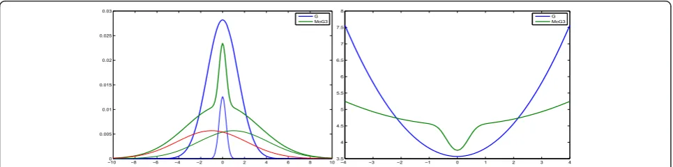
2.9 Mixture of three Gaussians (MoG3) model

Another mixture model proposed is using a Mixture of three Gaussians, one centered at zero and two symme-trically placed:

p(f|λ,v0,v+1,v−1,β) =

j

(1−λ)N(fj|0,v0)

+ (λ/2)N(fj|+β,v+1) +(λ/2)N(fj|−β,v−1)

(32)

which can also be expressed through the ternary valued hidden variableszjÎ{-1, 0, +1}

⎧ ⎪ ⎪ ⎪ ⎨ ⎪ ⎪ ⎪ ⎩

p(f|z) =_jp(fjzj) =

jN(fjzjβ,vzj)

P(zj= 1) =λ/2, P(zj=−1) =λ/2, P(zj= 0) = 1−λ.

(33)

In generalv+1=v-1 =v>>v0and lmeasures the spar-sity (0 <l<< 1). This family of models are illustrated on Figure 13.

−010 −8 −6 −4 −2 0 2 4 6 8 10

0.005 0.01 0.015 0.02 0.025 0.03

G MoG2

−4 −3 −2 −1 0 1 2 3 4

3.5 4 4.5 5 5.5 6 6.5 7 7.5 8

G MoG2

Figure 11Mixture of two Gaussians family. The probability density functionp(x) is shown in the left and - lnp(x) is shown in the right.

−010 −8 −6 −4 −2 0 2 4 6 8 10

0.02 0.04 0.06 0.08 0.1 0.12

G MoG2

−4 −3 −2 −1 0 1 2 3 4

2 3 4 5 6 7 8

G MoG2

2.10 Mixture of one Gaussian and two Gammas (MoGGammas) model

Another mixture model proposed is using a mixture of one central Gaussian and two symmetric Gammas:

p(f|λ,v0,α,β) =

j

(1−λ)N(fj|0,v0)

+ (λ/2)G(fj|α,β) +(λ/2)G(−fj|α,β)

(34)

which can also be expressed through the ternary valued hidden variableszjÎ{-1, 0, +1}

⎧ ⎪ ⎪ ⎪ ⎪ ⎪ ⎪ ⎪ ⎨ ⎪ ⎪ ⎪ ⎪ ⎪ ⎪ ⎪ ⎩

p(f|z) =_j(fjzj) = [N(fj|0,v0)]

jδ(zj)×

[G(fj|α,β)]

jδ(zj−1)×

[G(−fj|α,β)]

jδ(zj+1)

P(zj= 1) =λ/2, P(zj=−1) =λ/2, P(zj= 0) = 1−λ.

(35)

This family of models are illustrated on Figure 14.

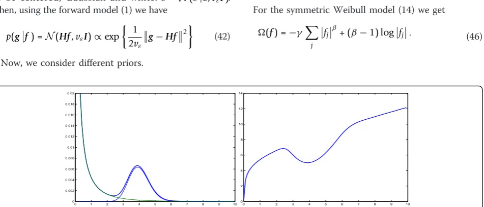
2.11 Bernoulli-Gamma (BGamma) model

As in the BG model, when we want to enforce both sparsity and positivity, we can use the BGamma model:

p(f|λ,α ,β) = j

[λδ(fj) + (1−λ)G(fj|α,β)] ₍₃₆₎

or ⎧ ⎪ ⎪ ⎨ ⎪ ⎪ ⎩

p(f|z) =

jp(fjzj) =

j[zjG(fj|α,β)]

j

(1−zj)δ(fj)

P(zj= 1) =λ, P(zj= 0) = 1−λ

(37)

A particular case of this model is Bernoulli-exponen-tial (BExponenBernoulli-exponen-tial) which obtained when a = 1. These families of models are illustrated on Figure 15 and Fig-ure 16.

2.12 Mixture of Dirichlet (MoD) model

•Mixture of Dirichlet model

p(f|λ,α1,α2) =λD(f|α1) + (1−λ)D(f|α2) (38)

where

D(f|α)∝ j

f_jα−1withfj>0,

j

fj= 1 ₍₃₉₎

is the symmetric Dirichlet distribution. We need to choose a1 > 1 for dense part and 0 <a2 < 1 for the sparse part.

2.13 Bernoulli-multinomial (BMultinomial) model

As in the BG or BGamma model, when we know that the signal is sparse and can only take one of the K

−010 −8 −6 −4 −2 0 2 4 6 8 10

0.005 0.01 0.015 0.02 0.025 0.03

G MoG3

−4 −3 −2 −1 0 1 2 3 4

3.5 4 4.5 5 5.5 6 6.5 7 7.5 8

G MoG3

Figure 13Mixture of three Gaussians family. The probability density functionp(x) is shown in the left and - lnp(x) is shown in the right.

−010 −8 −6 −4 −2 0 2 4 6 8 10

0.005 0.01 0.015 0.02 0.025 0.03

G MoGGammas

−4 −3 −2 −1 0 1 2 3 4

3.5 4 4.5 5 5.5 6 6.5 7 7.5 8

G MoGGammas

discrete values {a1, ..., aK}, we can use the BMultinomial

model:

p(f|λ,a,α) = j

λMult(fj|a,α) + (1−λ)δ(fj) ₍₄₀₎

wherea= {a1, ...,aK} anda= {a1, ...,aK} with∑kak=

1 and

Mult(fj|a,α) = n! a1!. . .aK!

k αaj

k

or ⎧ ⎪ ⎨ ⎪ ⎩

p(f|z) =_jp(fjzj) =

j

zjMult(fj|α)

j

(1−zj)δ(fj)

P(zj= 1) =λ, P(zj= 0) = 1−λ

(41)

3 Bayesian inference with sparsity enforcing priors

The priors proposed can be used in a Bayesian approach to infer onfgiven the observed datagthrough the poster-ior law given in Equation (3). First let assume the error to be centered, Gaussian and white: ε∼N(ε|0,v_εI). Then, using the forward model (1) we have

p(gf) =N(Hf,v_εI)∝exp

1

2v_εg−Hf 2

(42)

Now, we consider different priors.

3.1 Simple prior models

Given p(g|f) and any simple prior law p(f), the posterior law is written:

p(fg)∝p(gf)p(f)∝exp{J(f)} (43) with

J(f) = 1

2v_εg−Hf 2

+(f) (44)

where Ω(f) = -ln p(f) and so the Maximum A Poster-iori (MAP) solution is expressed as the minimizer of this criterion which has two parts: the first part is due to the likelihood and the second part is due to the prior:

Thus, depending on the choice of the prior we obtain different expressions forΩ(f). For example for the GG model of (10) we get

(f) =γ j

fjβ). ₍₄₅₎

For the symmetric Weibull model (14) we get

(f) =−γ j

fjβ+ (β−1) logfj. ₍₄₆₎

0 1 2 3 4 5 6 7 8 9 10

0 0.02 0.04 0.06 0.08 0.1 0.12

BG: lambda=.1;alpha=2;beta=1;

0 1 2 3 4 5 6 7 8 9 10

2 3 4 5 6 7 8 9 10 11

Figure 15Bernouilli-Gamma family. The probability density functionp(x) is shown in the left and - lnp(x) is shown in the right.

0 1 2 3 4 5 6 7 8 9 10

0 0.002 0.004 0.006 0.008 0.01 0.012 0.014 0.016 0.018 0.02

0 1 2 3 4 5 6 7 8 9 10

0 2 4 6 8 10 12 14

For the Student-t model (17) we get

(f) = ν+ 1 2

j

log(1 +f_j2/v). ₍₄₇₎

For the elastic net model we get

(f) =

j

γ1fj+γ2fj2

(48)

and for the Dirichlet model we get

(f) =

j

f_jα−1, fj>0,

j

fj= 1. ₍₄₉₎

For each of these cases, we may discuss on the unim-odality and convexity of the criterionJ(f) which depends mainly on its Hessian

J(f) =

∂2_J(f) ∂fj∂fi

=HH+

∂2_(f) ∂fi∂fj

=HH+

!

∂2_(f) ∂f2

j

" (50)

We may look at each case to examine the range of the parameters for which this Hessian matrix is positive definite.

The optimization is done iteratively:

Update operation can be additive, multiplicative or more complex. Updating stepsa(k)can be fixed or com-puted adaptively at each step (steepest descent for example).δf(k)can be, for example proportional to the gradient, in which case, we have

We may also consider to estimate some of these para-meters by assigning them appropriate priors and then express the jointp(f,θ|g,θ0) as given in Equation (4) and then try to estimate them jointly, for example joint MAP:

or alternate optimization:

We may also want to explore this joint posterior by generating samples from it. This can be done, for exam-ple, through the following Gibbs sampling scheme:

When a great number of samples are thus generated, we may compute their means, variances or any other statistics about them.

Finally, we may try to approximate this joint posterior by a simpler one, for example by a separableq(f,θ) =q1 (f)q2(θ) using the variational approximation (VA). The main idea and the main basic steps to achieve this is more detailed in the following section. Here, however, we present the result on the following scheme:

To illustrate the differences, we may consider the sim-ple case of a linear forward model and Gaussian priors:

p(gf,v_ε) =N(Hf,v_εI)

p(fvf) =N(0,vfI) (51)

In this case, if we knowθ= (v, vf), then

p(fg,v_ε,vf) =N(μ,) with:

μ= [HH+λI]−1Hg

= [HH+λI]−1

(52)

with λ= v_vε

f. So, we have f =μ which can be

Now putting inverse Gamma priors onv and vf, or

equivalently Gamma priors onτ= 1/v andτf= 1/vf:

p(τε|ατ0,βτ0) =G(αε0,βε0)

p(τfαf0,βf0) =G(αf0,βf0) (53)

we have

p(τ_εf,g,α_τ0,βτ0) =G(αε,βε)

p(τff,αf0,βf0) =G(αf,βf)

(54) with ⎧ ⎪ ⎪ ⎪ ⎪ ⎪ ⎪ ⎪ ⎪ ⎪ ⎪ ⎪ ⎨ ⎪ ⎪ ⎪ ⎪ ⎪ ⎪ ⎪ ⎪ ⎪ ⎪ ⎪ ⎩

αε=αε0+ 1/2

βε=βε0+g−Hf 2

/2

τε=ατ/βτ= 2αε0+ 1 2βε0+g−Hf

2

αf =αf0+ 1/2

βf =βf0+f 2

/2

τf =βf/αf =

2αf0+ 1 2βf0+f

2

(55)

and λ=τf

τε. Then, the alternate optimization of the JMAP estimate algorithm becomes

The Gibbs sampling algorithm becomes

The VBA algorithm becomes ⎧ ⎪ ⎪ ⎪ ⎪ ⎪ ⎪ ⎪ ⎪ ⎪ ⎪ ⎪ ⎪ ⎪ ⎪ ⎪ ⎪ ⎪ ⎪ ⎪ ⎪ ⎪ ⎪ ⎪ ⎪ ⎪ ⎪ ⎨ ⎪ ⎪ ⎪ ⎪ ⎪ ⎪ ⎪ ⎪ ⎪ ⎪ ⎪ ⎪ ⎪ ⎪ ⎪ ⎪ ⎪ ⎪ ⎪ ⎪ ⎪ ⎪ ⎪ ⎪ ⎪ ⎪ ⎩

q(f) =N(μ,)

= [HH+λI]−1

μ=Hg

q(τ_ε) =G(α_ε,β_ε)

αε=αε0+ 1/2

βε=βε0+g−H<f > 2

/2

q(τf) =G(αf,βf)

αf =αf0+ 1/2

βf =βf0+ 1 2

f2=βf0+ 1 2

jf 2 j

<f>=μ

f2=μ2+ diag

(56)

andλ=τf

τε:

We recently implemented these algorithms for differ-ent applications such as: synthetic aperture radar (SAR) Imaging [29], ...

3.2 Mixture models

For the mixture models, and in general for the models which can be expressed via the hidden variables, we want to estimate jointly the original unknownsfand the hidden variables: τin Cauchy model,zin MoG2, BG or

BGam models and zin MoG3 or MoGGammas. Let

examine these a little in details.

3.3 Student-t and Cauchy models

In this case the joint prior law can be written as:

p(f,τ) =

jp(fjτj)p(τj) =

jN(fj0, 1/τj)p(τj) ∝exp

−1 2

jτjf 2

j +alnτj−bτj

witha = b=ν/2

(57)

such that

p(f,τg)∝p(gf)p(f,τ)∝exp{−J(f,τ)} (58) where

j(f,τ) = 1

2v_εg−Hf 2

+

j 1 2τjf

2

j −alnτj+bτj ₍₅₉₎

Joint optimization of this criterion, alternatively with respect tof (with fixedτ)

_{f = arg minf{J(f,τ)}}

= arg minf

1

2vεg−Hf

2

+

j 1 2τjf

2 j

₍₆₀₎

and with respect toτ (with fixedf)

τ = arg min_τ{J(f,τ)}

= arg min_τ j

1 2τjf

2

j −alnτj+bτj

results in the following iterative algorithm: ⎧

⎪ ⎪ ⎨ ⎪ ⎪ ⎩

_{f = [HH+v}

εD(τ)]−1Hg

τj=φ(fj) = a

f_j2+b

D(τ) = diag[1/τj,j= 1, ...,n]

(62)

Note that, τjis the inverse of a variance and we have

1/τj= f_j2+b

a . We can interpret this as an iterative

quad-ratic regularization inversion followed by the estimation of variances τj which are used in the next iteration to

define the variance matrixD(τ).

Here too, we may study the conditions on which the joint criterion is uni-modal and its alternate optimiza-tion converges to its unique soluoptimiza-tion.

We may also consider a Gibbs sampling scheme

f∼p(fτ,g)∝p(gf)p(f|u) =N(ff,)

τ∼p(τf,g)∝p(f|τ)p(τ) =_jG(τjα,β)

(63)

where

= [HH+vεD(τ)]−1

_{f =}Hg (64)

and

α= 1 2fj+a=

1 2fj+ν/2

β=b =ν/2

(65)

For the VBA, we have ⎧

⎪ ⎪ ⎪ ⎪ ⎨ ⎪ ⎪ ⎪ ⎪ ⎩

p(gf,vε) =N(gHf,vεI), τε= 1/vε

p(τε) =G(τε|αε0,βε0) p(f|v) =_jp(fjvj) =

jN(fj0,vj) =N(f|0,V) V= diag[v], τj= 1/vj, τ = diag[τ] =V−1 p(τ) =_jG(τj|α0,β0)

(66)

⎧ ⎨ ⎩

q(f) =N(fμ,)

μ=Hg

= (τ_εHH+V)−1, withV= diag[v]

(67)

⎧ ⎪ ⎪ ⎪ ⎪ ⎪ ⎪ ⎪ ⎪ ⎪ ⎪ ⎨ ⎪ ⎪ ⎪ ⎪ ⎪ ⎪ ⎪ ⎪ ⎪ ⎪ ⎩

q(τ_ε) =G(τ_ε|α_ε,β_ε),

αε=αε0+ (n+ 1)/2

βε=βε0+ 1/2

τ =α_τ/β_τ

q(τj) =G(τjαj,βj)

αj=α00+ 1/2

βj=β00+<fj2>/2

zj=βj/αj

(68)

3.4 Mixture of two Gaussians (MoG2) model

In this case, following the same arguments, we obtain:

p(f,zg)∝p(gf)p(f,z)∝exp{−J(f,z)} (69) where

J(f,z) = 1 2vε

g−Hf2

+

j f2

j 2vzj

+zjlnλ+ (1−zj) ln(1−λ)

(70)

Again, in this case also, the optimization of this criter-ion, alternatively with respect to f and zresults in the following iterative algorithm:

⎧ ⎪ ⎪ ⎪ ⎪ ⎪ ⎨ ⎪ ⎪ ⎪ ⎪ ⎪ ⎩

_{f = [HH+vεD(z)]}−1 Hg

zj=φ(fj) =

⎧ ⎪ ⎨ ⎪ ⎩

1, iff2

j ≥(v1−v0) ln 1−λ

λ 0, iff2

j <(v1−v0) ln 1−λ

λ D(z) = diagvzj,j= 1, ..,n

(71)

Here too, we may also consider a Gibbs sampling scheme

f∼p(fz,g)∝p(gf)p(f|u) =N(ff,) z∼p(zf,g)∝p(f|z)p(z) =_jP(zj=kfj)

(72)

where

= [HH+vεD(z)]−1

and ⎧ ⎪ ⎨ ⎪ ⎩

P(zj= 1fj) = 1, iffj2≥(v1−v0) ln 1−λ

λ P(zj= 0fj) = 1, iffj2<(v1−v0) ln

1−λ λ

(74)

3.5 BG model

For the case of BG we have to be more careful, because the joint probability laws are degenerated. Two approaches are then possible:

i) Considering them as the particular case of the MoG models where the variancev0 is fixed to a small value or reduced gradually during the iterations.

ii) Trying first to integrate outf from the expression ofp(f, z|g) to obtainp(z|g) and optimize it with respect toz(detection step) and then use it for the estimation step.

To go further in detail of the second approach, we may remark that for the givenz, the expression of p(f,

z|g) as a function of fis Gaussian and so it can be easily integrated out and we obtain:

p(zg)∝p(g|z)p(z)

∝N(g|0 ,H(vdiag[zj,j= 1,...,n])H+vεI)× λjzj₍₁−λ₎j(1−zj)

(75)

Now writing the expression ofL(z) =−lnp(zg)and keeping only all terms depending onzwe obtain:

L(z) =−gB−1(z)g−lnB(z)−2nln1−λ

λ (76)

whereB(z) = H(vdiag [zj,j= 1, ...,n])H’+vI. We see

the complexity of this expression which needs the inver-sion of the matrix B and its optimization which is a combinatorial optimization needing to evaluate this expression 2ntimes.

However, we may also remark that when zobtained, the estimation offis easy. We have:

_{f =HB}−1_{g. (77)}

which needs again the inversion of the matrixB. The exact computations of z and f are often too costly, one may try to obtain approximate solutions. Many approximations have been proposed. A good overview of these methods can be found in [30, Chap. 5] and also in [31,32].

3.6 BGamma and MoGGammas model

In these cases, it is no more possible to integrate outf analytically as it was the case with Gaussians. One strat-egy here is to use the MCMC methods to generate sam-ples from the joint posterior. The second approach is to approximate the joint posterior by a simpler one, for example by a separable one on f and the hidden vari-ableszin the BGamma or the MoGGammas cases. Very often then we can do the computations analytically. However, it may happens that, even after these separable approximations, still we need to use the MCMC meth-ods on some of variables. Detailed explanation of these general methods is out of focus of this article. See [30,33,34]. Here, we just give the details for the case of the Gaussian mixtures (MoG2 or MoG3).

4 Variational Bayesian approximation for the case of mixture laws

To start and to be complete as to propose an unsupervised method, we include also the estimation of the parameters

θand write the joint posterior law of all the unknowns:

p(f,z,θg)∝p(gf,θ)p(f|z,θ)p(z|θ)p(θ) (78) which can also be written as

q(f,z,θg) =p(fz,θ;g)p(zθ;g)p(θg) (79) where

p(f|z,θ;g) =p(gf,θ)p(f|z,θ)/p(g|z,θ) (80) with

p(g|z,θ) =

p(gf,θ)p(f|z,θ) df

and

p(zθ;g) =p(g|z,θ)p(z|θ)/p(g|θ) (81) with

p(g|θ) =

p(g|z,θ)p(z|θ) dz

or

p(g|θ) = z

p(g|z,θ)p(z|θ)

whenzare discrete valued, and finally

p(θg) =p(g|θ)p(θ)/p(g) (82) with

p(g) =

One can also write:

p(zθ,g) =

p(f,zθ,g) df (83)

and

p(θg) = p(f,z,θg) df dz=

p(zθ;g) dz(84) or

p(θg) = z

p(f,z,θg) df = z

p(zθ;g) (85)

whenzare discrete valued. We see that the first term

p(fz,θ,g)∝p(gf,θ)p(f|z,θ) (86) will be easy to handle because it is the product of two Gaussians and so it is a multivariate Gaussian. But the two others are not.

The main idea behind the VBA is to approximate the joint posterior p(f,z,θ|g) by a separable one, for exam-ple

q(f,z,θg) =q1(fg)q2(zg)q3(θg) (87) illustrated here:

and where the expressions ofq(f,z,θ|g) is obtained by minimizing the Kullback-Leibler divergence

KL(q:p) =

qlnq p=

#

lnq p

$

q

(88)

It is then easy to show that

KL(q:p) = lnp(g|M)−F(q) (89)

wherep(g|M)is the likelihood of the model

p(g|M) =

p(f,z,θ,g|M) df dzdθ (90) with

p(f,z,θ,g|M) =p(gf,θ)p(f|z,θ)p(z|θ)p(θ) (91) andF(q)is the free energy associated toqdefined as

F(q) =

#

lnp(f,z,θ,g|M) q(f,z,θ)

$

q

(92)

So, for a given model M, minimizing KL(q : p) is equivalent to maximizing F(q)and when optimized, F(q∗)gives a lower bound forlnp(g|M).

Without any other constraint than the normalization of q, an alternate optimization ofF(q)with respect to q1,q2, andq3results in

q1(f)∝exp

−%lnp(f,z,θ,g)&_q(z)q(θ) q2(z)∝exp

−%lnp(f,z,θ,g)&_q(f)q(θ) q3(θ)∝exp

−%lnp(f,z,θ,g)&_q(f)q(z)

Note that these relations represent an implicit solution forq1(f), q2(z), and q3(θ) which need, at each iteration, the expression of the expectations in the right hand of exponentials. If p(g|f, z,θ1) is a member of an exponen-tial family and if all the priorsp(f|z, θ2),p(z|θ3),p(θ1),p (θ2), andp(θ3) are conjugate priors, then it is to see that these expressions leads to standard distributions for which the required expectations are easily evaluated. In that case, we may note

q(f,z,θg) =q1(fz,θ;g)q2(zf,θ;g)q3(θf,z;g)(93) where the tilded quantitiesz,f and_θ are, respectively functions of(f,θ), (z,θ)and(f,z):

and where the alternate optimization results to alter-nate updating of the parameters(z,θ)for q1, the para-meters(f,θ)ofq2 and the parameters(f,z)ofq3.

Finally, we may note that, to monitor the convergence of the algorithm, we may evaluate the free energy

F(q) =

#

lnp(f,z,θ,g|M) q(f,z,θ)

$

q

=%lnp(f,z,θ,g)|M&_q+%−lnq(f,z,θ)&_q =%lnp(gf,z,θ)&_q+%lnp(f|z,θ)&_q+%lnp(z|θ)&_q

+%−lnq(f)&_q+%−lnq(z)&_q+%−lnq(θ)&_q

(94)

Other decompositions are also possible:

q(f,z,θg) =q1(fz,θ;g)

jq2j(zj

f,z(−j),θ;g)

jq3l(θl

f,z,θ(−l);g)

(95)

illustrated here:

or even by:

q(f,z,θg) = jq1j(fj

f_(−j),z,θ;g)

jq2j(zj

f,z(−j),θ;g)

lq3l(θl

f,z,θ(−l);g)

(96)

illustrated here:

Here, we consider the second case (Equation (95)) and give some more details on it. First to simplify the nota-tions, we write it as:

q(f,z,θ) =q1(f)

j q2j(zj)

l

q3l(θl) ₍₉₇₎

where it can be shown that:

q1(f)∝exp

−%lnp(f,z,θ,g)&_q 2(z)q3(θ)

q2j(zj)∝exp

−%lnp(f,z,θ,g)&_q1(f)q

3(θ)q2(z(−j))

q3l(θl)∝exp

−%lnp(f,z,θ,g)&_q

1(f)q2(z)q3(θ(−l))

where p(f, z, θ, g) = p(g|f, θ)p(f|z, θ)p(z|θ)p(θ) and whereq2(z) = Πjq2j(zj),q3(θ) =Πlq3l(θl),q2(z(-j)) = Πi≠j q2j(zj),〈.〉qmeans expected value with respect toq.

In that case, with appropriate models for the priors (exponential families) and hyper parameters (conjugate priors), we see that q(f) is a multivariate Gaussian

g(f) =N(fμ,), q(θl) are either Gaussians (for the

means) or Inverse Gammas (for the variances) and q(zj)

are discrete distributions whose expressions can be writ-ten easily.

To illustrate this in more detail, we consider the case of the Student-t model.

4.1 Student-t model

In this case, we have the following relations for the for-ward model and the prior laws:

⎧ ⎪ ⎪ ⎪ ⎪ ⎨ ⎪ ⎪ ⎪ ⎪ ⎩

p(gf,vε) =N(gHf,vεI), τ= 1/vε

p(f|z) =jp(fjzj) =jN(zj0,zj) =N(f|0,Z)

Z= diag[z], aj= 1/zj, A= diag[a] =Z−1

p(a) =jG(aj|α0,β0)

p(τ) =G(τ|ατ0,βτ0)

(98)

Then, we obtain the following expressions for the VBA:

⎧ ⎨ ⎩

q(f) =N(fμ,)

μ=< τ >Hg

= (< τ >HH+Z)−1, withZ=A˜−1= diag[a]

(99) ⎧ ⎪ ⎪ ⎪ ⎪ ⎪ ⎪ ⎪ ⎪ ⎪ ⎪ ⎨ ⎪ ⎪ ⎪ ⎪ ⎪ ⎪ ⎪ ⎪ ⎪ ⎪ ⎩

q(τ) =G(τατ,βτ),

ατ=ατ0+ (n+ 1)/2

βτ=βτ0+ 1/2

g2−2<f >Hg+H<f f>H

q(aj) =G(ajαj,βj)

αj=α00+ 1/2

βj=β00+<fj2>/2

(100)

where the expressions of the expectations needed are: ⎧ ⎪ ⎪ ⎪ ⎪ ⎨ ⎪ ⎪ ⎪ ⎪ ⎩

<f>=μ <ff>=+μμ <f_j2>= []jj+μ2j < τ >=τ =α_τ/β_τ <aj>=aj=αj/βj

(101)

We can also express the free energy expression:

F(q) =

#

lnp(f,a,τ,g|M) q(f,a,τ)

$

=%lnp(gf,a,τ)&+%lnp(f|a,τ)&+%lnp(a|τ)& +%−lnq(f)&+%−lnq(a)&+%−lnq(τ)&

(102)

where %

lnp(gf,τ)&= n 2

'

<lnτ >−ln(2π)(

−1 2

)

< τ >gg−2<f >Hg+H<ff>H*

%

−lnp(f |a)&=−n+ 1 2 ln(2π)

−1 2

j<lnαj>< αj><f 2 j >

%

−lnp(a)&=−(n+ 1)αε0ln(βε0) + (αε0−1)

j[<lnαj>−β < αj)]−(n+ 1) ln(α)

%

and %

−lnq(f)&=−n+ 1

2 (1 + ln(2π))− 1 2lnj

%

−lnq(a)&=− j

αjln(βj) + (αj−1)<lnαj> −βj< αj>−ln(αj)

%

q(τ))&=c˜lnd˜+ (˜c−1)<lnτ)>−˜d< τ >−ln(˜c)

In these equations, ⎧

⎪ ⎪ ⎨ ⎪ ⎪ ⎩

<lnaj>=ψ(˜aj)−lnb˜j <lnτ >=ψ(˜c)−lnd˜ ψ(a) = ∂ln(a)

∂a

(103)

The resulting algorithm can be summarized as follows

5 Conclusion

The sparsity is a required property in many signal and image processing applications. In this article, first we reviewed the main steps of the Bayesian approach for inverse problems in signal and image processing. Then we presented in a synthetic way the different prior mod-els which can be used to enforce the sparsity. These models have been presented in two categories: simple and hierarchical with hidden variables. For each of these prior models, we discuss their properties and the way to use them in a Bayesian approach resulting to many dif-ferent inversion algorithms.

We have applied these Bayesian algorithms in many different applications such as X-ray computed tomogra-phy [35,36], optical diffraction tomogratomogra-phy [37-39], posi-tron emission tomography [40], Microwave imaging [41,42], Sources separation [43-46], spectrometry [47,48], Hyper spectral imaging [49], super resolution [50-52], image fusion [53], image segmentation [54], synthetic aperture radar (SAR) imaging [29]. To save the place and be very synthetic, we did not give here any simulation results or any results on different appli-cations of these methods. These can be found in differ-ent articles just referenced.

Acknowledgements

This study had been partially founded by the C5Sys project (Circadian and Cell cycle Clock systems in Cancer) of ERASYSBIO+. http://www.erasysbio. net/index.php?index=272

Competing interests

The author declares that they have no competing interests.

Received: 18 January 2012 Accepted: 1 March 2012 Published: 1 March 2012

References

1. A Tikhonov, Regularization of incorrectly posed problems. Soviet Math Dokl.

4, 1624–1627 (1963)

2. A Tikhonov, V Arénine, Méthodes de Résolution de Problémes Mal Posés,

(MIR, Moscu, Russia, 1976). ?É?ditions

3. I Daubechies, M Defrise, CD Mol, An iterative thresholding algorithm for linear inverse problems with a sparsity constraint. Comm Pure Appl Math.

57, 1413–1457 (2004). doi:10.1002/cpa.20042

4. DL Donoho, Compressive sampling. IEEE Trans Inf Theory.52(4), 1289_–1306 (2006)

5. JA Tropp, AC Gilbert, MJ Strauss, Algorithms for simultaneous sparse approximation. Part I: Greedy pursuit. Signal Processing, special issue“sparse approximations in signal and image processing”.86, 572–588 (2006) 6. JA Tropp, Algorithms for simultaneous sparse approximation. Part II: Convex

relaxation. Signal Process (special issue“Sparse approximations in signal and image processing_”).86, 589_–602 (2006)

7. R Zass, A Shashua, inNonnegative Sparse PCA, vol. 19. (Cambridge, MA: MIT Press, 2007), pp. 1561_–1568

8. EJ Candés, M Wakin, S Boyd, Enhancing sparsity by reweighted l1 minimization. J Fourier Anal Appl.14, 877–905 (2008). doi:10.1007/s00041-008-9045-x

9. DM Witten, R Tibshirani, T Hastie, A penalized matrix decomposition, with applications to sparse principal components and canonical correlation analysis. Biostatistics.10(3), 515–534 (2009). doi:10.1093/biostatistics/kxp008 10. S Vaiter, G Peyré, C Dossal, J Fadili, Robust Sparse Analysis Reg-ularization.

Tech rep, preprint Hal-00627452 http://hal.archives-ouvertes.fr/hal-00627452/ (2011)

11. G Peyré, J Fadili, Learning Analysis Sparsity Priors. Proc of Sampta’11 http:// hal.archives-ouvertes.fr/hal-00542016/ (2011)

12. P Williams, Bayesian regularization and pruning using a Laplace prior. Neural Comput.71, 117–143 (1995)

13. T Mitchell, J Beauchamp, Bayesian variable selection in linear regression. J Am Stat Assoc.83(404), 1023 (1988). doi:10.2307/2290129

14. N Polson, J Scott, Shrink globally, act locally: sparse Bayesian regulariza-tion and prediction. Bayesian Stat.9, 1–24 (2010)

15. A Mohammad-Djafari, On the estimation of hyperparameters in Bayesian

approach of solving inverse problems, inProc IEEE International Conference on Acoustics, Speech, and Signal Processing ICASSP-93, vol. 5. (Minneapolis, MN, USA, 1993), pp. 495–498

16. A Mohammad-Djafari, Joint estimation of parameters and hyperparameters

in a Bayesian approach of solving inverse problems, inIEEE Int Conf on Image Processing (ICIP), IEEE ICIP 96, vol. II. (Lausanne, Swisse, 1996), pp. 473–477

17. R Neal, G Hinton, A view of the EM algorithm that justifies incremental, sparse, and other variants. Learn Graph Models.89, 355_–368 (1998) 18. A Doucet, P Duvaut, Bayesian estimation of state-space models applied to

deconvolution of Bernoulli-Gaussian processes. Signal Process.57(2), 147–161 (1997). doi:10.1016/S0165-1684(96)00192-2

19. T Park, G Casella, The Bayesian Lasso. J Am Stat Assoc.103(482), 681_–686 (2008). doi:10.1198/016214508000000337

20. M Tipping, Sparse Bayesian learning and the relevance vector machine. J Mach Learn Res.1, 211–244 (2001)

21. C Févotte, S Godsill, A Bayesian aproach for blind separation of sparse source. IEEE Trans Audio Speech Lang Process.14, 2174–2188 (2006) 22. F Caron, A Doucet, Sparse Bayesian nonparametric regression, in

International Conference on Machine Learning, pp. 88_–95 (2008) 23. J Griffin, P Brown, Inference with normal-gamma prior distributions in

regression problems. Bayesian Anal.5, 171_–188 (2010)

24. H Snoussi, J Idier, Bayesian blind separation of generalized hyperbolic processes in noisy and underdeterminate mixtures. IEEE Trans Signal Process.54, 3257–3269 (2006)

25. H Ishwaran, JS Rao, Spike and slab variable selection: frequentist and Bayesian strategies. Ann Stat.33(2), 730–733 (2005). doi:10.1214/ 009053604000001147

27. CA Bouman, KD Sauer, A generalized Gaussian image model for edge-preserving MAP estimation. IEEE Trans Image Process.2(3), 296_–310 (1993). doi:10.1109/83.236536

28. H Zou, T Hastie, Regularization and variable selection via the elastic net. J Royal Stat Soc, Ser, B.67(2), 301–320 (2005). doi:10.1111/j.1467-9868.2005.00503.x

29. S Zhu, A Mohammad-Djafari, H Wang, B Deng, X Li, J Mao, Parameter

estimation for SAR micromotion target based on sparse signal representation. Eurasip special issue“Sparse approximations in signal and image processing”.13(2012)

30. J Idier, Approche Bayésienne Pour les Problémes Inverses,(Traité IC2, Série traitement du signal et de l’image, Hermés, Paris, 2001)

31. F Champagnat, Y Goussard, J Idier, Unsupervised deconvolution of sparse spike trains using stochastic approximation. IEEE Trans Signal Process.

44(12), 2988_–2998 (1996). doi:10.1109/78.553473

32. D Ge, J Idier, E Le Carpentier, A new MCMC algorithm for blind Bernoulli-Gaussian deconvolution, Proceedings of EUSIPCO: Septembre 2008, (Lausanne, Suisse, 2008)

33. JJ Kormylo, JM Mendel, Maximum-likelihood detection and estimation of Bernoulli-Gaussian processes. IEEE Trans Inf Theory.28, 482–488 (1982). doi:10.1109/TIT.1982.1056496

34. M Lavielle, Bayesian deconvolution of Bernoulli-Gaussian processes. Signal Process.33, 67–79 (1993)

35. A Mohammad-Djafari, Gauss-Markov-Potts priors for images in computer

tomography resulting to joint optimal reconstruction and segmentation. Int J Tomography Stat.11(W09), 76_–92 http://djafari.free.fr/pdf/IJTS 08.pdf (2008)

36. N Gac, A Vabre, A Mohammad-Djafari, F Buyens, GPU implementation of a

3D bayesian CT algorithm and its application on real foam reconstruction, Proceedings of the first International Conference on Image Formation in X-Ray Computed Tomography,(Salt Lake City, Utah, USA, 2010)

37. H Ayasso, B Duchne, A Mohammad-Djafari, Bayesian inversion for optical diffraction tomography. J Modern Opt.57(9), 765_–776 (2010). doi:10.1080/ 09500340903564702

38. H Ayasso, A Mohammad-Djafari, Joint NDT image restoration and

segmentation using Gauss-Markov-Potts prior models and variational Bayesian computation. IEEE Trans. Image Process.19(9), 2265_–2277 http:// dx.doi.org/10.1109/TIP.2010.2047902 (2010)

39. H Ayasso, B Duchne, A Mohammad-Djafari, Optical diffraction tomography

within a variational Bayesian framework. Inverse Probl Sci Eng.iFirst, 1–15 (2011)

40. MD Fall, ?É? Barat, C Comtat, T Dautremer, T Montagu, A

Mohammad-Djafari, A discrete-continuous Bayesian model for emission tomography, IEEE International Conference on Image Processing (ICIP),(Bruxell, Belgium, 2011), pp. 1401–1404

41. O Féron, B Duchêne, A Mohammad-Djafari, Microwave imaging of

inho-mogeneous objects made of a finite number of dielectric and conductive materials from experimental data. Inverse Probl.21(6), 95_–115 http://djafari. free.fr/pdf/ (2005). doi:10.1088/0266-5611/21/6/S08

42. O Féron, B Duchêne, A Mohammad-Djafari, Microwave imaging of

piece-wise constant objects in a 2D-TE configuration. Int J Appl Electromag Mech.

26(6), 167–174 http://djafari.free.fr/pdf/jae00905.pdf (2007)

43. H Snoussi, A Mohammad-Djafari, Fast joint separation and segmentation of mixed images. J Electron Imag.13(2), 349–361 http://djafari.free.fr/pdf/ (2004). doi:10.1117/1.1666873

44. H Snoussi, A Mohammad-Djafari, Bayesian unsupervised learning for source separation with mixture of Gaussians prior. J VLSI Signal Process Syst.37(2/ 3), 263–279http://djafari.free.fr/pdf/VLSIpapar.pdf (2004)

45. A Mohammad-Djafari, Bayesian source separation: beyond PCA and ICA, in

ESANN 2006, (Belgium, 2006) http://djafari.free.fr/pdf/

46. M Ichir, A Mohammad-Djafari, Hidden Markov models for wavelet-based

blind source separation. IEEE Trans Image Process.15(7), 1887–1899 (2006) 47. A Mohammad-Djafari, J Giovannelli, G Demoment, J Idier, Regulariza-tion,

maximum entropy and probabilistic methods in mass spectrometry data processing problems. Int J Mass Spectrom.215(1-3), 175–193 http://djafari. free.fr/pdf/maspec12013.pdf (2002). doi:10.1016/S1387-3806(01)00562-0 48. S Moussaoui, D Brie, A Mohammad-Djafari, C Carteret, Separation of

non-negative mixture of non-non-negative sources using a Bayesian approach and MCMC sampling. IEEE Trans Signal Process.54(11), 4133–4145 (2006)

49. N Bali, A Mohammad-Djafari, Bayesian approach with hidden Markov

modeling and mean field approximation for hyperspectral data analysis. IEEE Trans Image Process.17(2), 217–225 (2008)

50. F Humblot, A Mohammad-Djafari, Super-resolution using hidden Markov

model and bayesian detection estimation framework, inEURASIP J Appl Signal Process, vol. 16. (Special number on Super-Resolution Imaging: Analysis, Algorithms, and Applications, 2006) http://www.hindawi.com/ GetArticle.aspx?doi=10.1155/ASP/2006/36971. Article ID 36971

51. A Mohammad-Djafari, Super-resolution: a short review, a new method

based on hidden Markov modeling of HR image and future challenges. Comput J http://djafari.free.fr/pdf/bxn005v1.pdf (2008)

52. M Mansouri, A Mohammad-Djafari, Joint super-resolution and segmentation

from a set of low resolution images using a Bayesian approach with a Gauss-Markov-Potts prior. Int J Signal Imag Syst Eng.3(4), 211–221 (2010). doi:10.1504/IJSISE.2010.038017

53. O Féron, A Mohammad-Djafari, Image fusion and joint segmentation using

an MCMC algorithm. J Electron Imag.14(2) http://arxiv.org/abs/physics/ 0403150 (2005). paper no. 023014

54. P Brault, A Mohammad-Djafari, Unsupervised Bayesian wavelet domain

segmentation using a Potts-Markov random field modeling. J Electron Imag.14(4) http://djafari.free.fr/pdf/ (2005). 043011-1-043011-16

doi:10.1186/1687-6180-2012-52

Cite this article as:Mohammad-Djafari:Bayesian approach with prior models which enforce sparsity in signal and image processing.EURASIP Journal on Advances in Signal Processing20122012:52.

Submit your manuscript to a

journal and benefi t from:

7Convenient online submission 7Rigorous peer review

7Immediate publication on acceptance 7Open access: articles freely available online 7High visibility within the fi eld

7Retaining the copyright to your article