INVESTIGATION
A Bayesian Nonparametric Approach for Mapping
Dynamic Quantitative Traits
Zitong Li* and Mikko J. Sillanpää†,‡,1
*Department of Mathematics and Statistics, University of Helsinki, Helsinki FIN-00014, Finland,†Department of Mathematical Sciences and Department of Biology, University of Oulu, Oulu FIN-90014, Finland, and‡Biocenter Oulu, Oulu, FIN-90014, Finland
ABSTRACT In biology, many quantitative traits are dynamic in nature. They can often be described by some smooth functions or curves. A joint analysis of all the repeated measurements of the dynamic traits by functional quantitative trait loci (QTL) mapping methods has the benefits to (1) understand the genetic control of the whole dynamic process of the quantitative traits and (2) improve the statistical power to detect QTL. One crucial issue in functional QTL mapping is how to correctly describe the smoothness of trajectories of functional valued traits. We develop an efficient Bayesian nonparametric multiple-loci procedure for mapping dynamic traits. The method uses the Bayesian P-splines with (nonparametric) B-spline bases to specify the functional form of a QTL trajectory and a random walk prior to automatically determine its degree of smoothness. An efficient deterministic variational Bayes algorithm is used to implement both (1) the search of an optimal subset of QTL among large marker panels and (2) estimation of the genetic effects of the selected QTL changing over time. Our method can be fast even on some large-scale data sets. The advantages of our method are illustrated on both simulated and real data sets.
I
N quantitative trait loci (QTL) mapping, people are typically interested infinding genomic positions influencing a single quantitative trait. When the repeated measurements over time of a developmental trait (such as body weight, milk produc-tion, and mineral density) are available, it is often preferable to analyze all dynamic time points (traits) jointly to obtain a better understanding of the genetic control of the trait over time (Wu and Lin 2006). To analyze such kinds of time course data, one simple possibility is to apply some multiple-trait methods (jointly analyze many unordered correlated traits) based on multivariate regression (Jiang and Zeng 1995; Banerjeeet al.2008). However, the standard multivariate re-gression often fails to model the specific dependent (order) structure in the dynamic phenotype data. In statistics, the order nature of the time course data (i.e., smoothness prop-erty) means that the two nearby measurements should have closer values than the two with farther distances. Regarding the smoothness assumption in the data, the following twodifferent improved statistical approaches have been used for the dynamic trait analysis:
i. Combining phenotypes: The phenotypic information over time points is combined by using some smoothing and/or data reduction techniques, and the combined data are used as the new response data for mapping QTL. Some examples include Geeet al.(2003), Heuven and Janss (2010), Hurtadoet al.(2012), and Sillanpääet al.(2012). Theyfirst fitted the repeated measures of the phenotype data at each individual by the logistic growth curve or a high-order poly-nomial curve, and next they used the estimated curve parameters for all the individuals as the latent trait data in a multivariate Bayesian regression model for mapping QTL. Outside the genetics context, Meier and Bühlmann (2007) proposed a combined-likelihood approach, where theyfirst reweighted the time course response variables by kernel smoothing techniques and then performed univariate regression (with a single response variable) independently on each reweighted response.
ii. Combining genetic effects: In a multiple-trait model, the parameters of the QTL effects (genotypic value) (i.e., time-varying coefficients) are reparameterized by specifying them as a smooth function over time. When the dynamic pattern of the trait is simple, the effects of a QTL over time can be specified as a parametric function (i.e., logistic
Copyright © 2013 by the Genetics Society of America doi: 10.1534/genetics.113.152736
Manuscript received April 30, 2013; accepted for publication June 5, 2013 Supporting information is available online athttp://www.genetics.org/lookup/suppl/ doi:10.1534/genetics.113.152736/-/DC1.
function). For such cases, Maet al. (2002) developed a maximum-likelihood-based approach. Alternatively, if the shape of the dynamic trait is complicated, one canfit the nonparametric curve, applying methods such as Legendre polynomials (Lin and Wu 2006; Yang and Xu 2007; Li
et al.2012), wavelets (Zhaoet al.2007), or B-splines (J. Yanget al.2009; R. Yang et al.2009; Xionget al.2011; Gong and Zou 2012; Xinget al. 2012). In addition, the residual terms of these models were often assumed to share a certain covariance structure such as an autoregres-sive process (Maet al.2002).
In this article, we concentrate on the second approach, which models the smoothness of the marker effects instead of the phenotype data. This might have the advantage of finding the real underlying dynamic pattern of QTL that characterize the developmental traits, so that we can easily interpret the results.
As for a single-trait QTL analysis, variable selection (i.e., choosing a subset of markers that can approximately repre-sent QTL) is an important issue also for mapping dynamic traits. Most of the existing frequentist approaches (Maet al.
2002; Lin and Wu 2006; Xionget al.2011; Gong and Zou 2012) follow single-locus functional mapping, which maps the dynamic traits to each marker one at a time and uses either likelihood methods or least-squares-estimating equa-tions approaches (with independent residual covariance structure). These approaches typically construct a test sta-tistic (e.g., log-likelihood ratio or Wald statistic) to screen the important variables (QTL) through a multiple-testing procedure (e.g., adjusting the P-value by permutation or by Bonferroni correction). In some Bayesian approaches (Yang and Xu 2007; Min et al. 2011; Yang et al. 2011; Li
et al.2012; Xinget al.2012), the multilocus QTL analysis is performed by assigning shrinkage-inducing priors or spike and slab priors to the marker effects. Wald tests, credible intervals (Liet al.2011), or Bayes factors can then be used to justify the QTL.
In this article, we develop a Bayesian multivariate re-gression method with smoothing prior settings for functional QTL mapping. In our model, we choose B-splines to repar-ameterize the time-varying marker effects. The benefit of using B-splines over Legendre polynomials, which have been intensively used for nonparametric modeling in some earlier functional mapping approaches, was explained in Xinget al.
(2012). Although both B-splines and Bayesian modeling have been considered in some earlier works listed above, our ap-proach has the following three new features. First, with B-splines, our focus is on automatic adaptive determination of the degree of smoothness (i.e., number of knots), which is a crucial problem in B-splines modeling. In the earlier works of Xionget al.(2011) and Gong and Zou (2012), the degree of smoothness of B-splines was chosen explicitly by cross-val-idation or the Akaike information criterion (AIC). While here we estimate the degree of smoothness implicitly by assigning second-order penalty priors (Fahrmeir and Kneib 2011) to
the time-varying parameters. In other words, we estimate the functional forms of the marker effects and infer their degrees of smoothness simultaneously. This could greatly sim-plify the whole estimation procedure. The original idea of such prior settings was introduced as P-splines (or B-splines with penalty) (Eilers and Marx 1996; Lang and Brezger 2004) and has been widely applied in the estimation prob-lems of the generalized additive models. Second, the above-mentioned Bayesian approaches were based on Markov chain Monte Carlo (MCMC) simulation, which could be computa-tionally inefficient for high-dimensional data with either a large number of markers or a large number of time points. Here, instead, we introduce a fast variational Bayes (Jaakkola and Jordan 2000; Beal 2003) approach for posterior esti-mation. Variational Bayes is a deterministic approximation method, which has been used in several single-trait QTL map-ping studies (Logsdonet al.2010; Carbonetto and Stephens 2012; Li and Sillanpää 2012). We generalize these ideas in a multivariate regression framework. Third, for model search or variable selection, we adopt a matching pursuit-like algo-rithm introduced in Nottet al.(2012) for a different context. The idea is similar to the well-known forward/backward se-lection (Hastieet al.2009; Seguraet al.2012), but it differs substantially from the Bayesian variable selection procedures used currently for Bayesian QTL mapping (e.g., Yang et al.
2011). The rest of the article is organized as follows: in Meth-ods, the concept of the (functional) multitrait model and B-splines is reviewed, and the prior settings, the variational Bayes algorithms, and the variable selection procedures are introduced; inExample analyses, we show the results of ana-lyzing two types of simulated data sets (including data repli-cates) and one real mouse data set (Xionget al.2011); and finally we summarize some key points of our functional ap-proach in theDiscussion.
Methods
Background
A multivariate Gaussian linear regression model for func-tional QTL mapping can be specified as
yiðtrÞ ¼b0ðtrÞ þ Xp
j¼1
xijbjðtrÞ þeiðtrÞ; (1)
for individuals i= 1,. . .,nand indexes of the time points
this article, we further assume that the residual covariance follows (i) an independent diagonal covariance structure S0¼diagðs21;. . .;s2kÞand (ii) a stationaryfirst-order autor-egressive [AR(1)] structure (Fahrmeir and Kneib 2011), which is defined as S0ðr;sÞ ¼s20rjr2sj=12r2 (0 , r ,1) for indexes of the time points r= 1,. . .,k,s= 1,. . .,k.
Remark:In principle, a QTL usually does not exactly locate at any marker position, but here we consider using a marker only to approximate the true QTL by assuming the high marker density (Xu 2003).
Note that the model (1) differs from some single-locus functional mapping approaches (Maet al.2002; Xionget al.
2011). Those authors specify the model for marker j (j= 1,. . ., p) as
yiðtrÞ ¼jij1gj1ðtrÞ þ
12jij1
gj2ðtrÞ þeiðtrÞ; (2)
wherejij1is the indicator of a particular genotype (e.g., AA) for markerjand individuali, andgj1(tr) andgj2(tr) are the corresponding genotypic values. Model (1) is different from (2). In (1), the multiple loci are included in the same equa-tion, and we assume no dominance effects.
A fundamental principle of functional mapping is that bj(tr)(j= 0,. . .,p), which is defined at discrete time points
tr(r= 1,. . .,k), actually comes from a continuous function bj(t) with the domaint2[t1,tk]. We may callbj(t) a trend function of the genetic effects since it describes how the effect size of a QTL changes over time. In this trend function, the smoothness property should hold, meaning that the nearby effects should share similar values. For instance, we may expect that the difference between bj(t1) and bj(t2) should be smaller than that between bj(t1) and bj(t3). Introducing smoothness for the time course data may have some advantage over the general methods for modeling multiple traits, where each bj(tr) (r = 1,. . .,k) is assumed to be independent from the other (Wu and Lin 2006). First, it could provide more biologically meaningful results, where we can directly see a dynamic pattern of a QTL contributing to the development of a trait. Second, when estimating the parameter at a particular time point, the information from the observations of the nearby time points can be shared, and this might be able to increase the statistical power to detect some true signals. One simple parametric way to model the smoothness is to specify a precise functional form tobj(t) over timetr. For example, Ma et al. (2002) specified it as a logistic function bjðtÞ ¼aj=ð1þbjexpð2cjtÞÞ, and estimated the parameters
aj,bj, andcjby maximum likelihood to determine the exact shape ofbj(t). The parametric method is simple and usually has only a small number of parameters to be estimated, but it is able to describe only a quite simple trend such as a monotonically increasing trend or, by other means, to describe a very smooth function with no function values changing abruptly at any time point. To model a more com-plicated dynamic pattern such as the irregular periodic trend
shown in the mouse active-state probability data (Xiong
et al.2011), some moreflexible nonparametric or semipara-metric methods such as basis expansions and kernels could be good alternatives (Hastie et al. 2009). Many functional mapping approaches are actually intensively based on basis expansions, which represent the additive genetic effectbj(t) as a linear combination ofmbasis functions as
bjðtÞ ¼X
m
h¼1
cjhðtÞajh; (3)
where the basis functionscjh(t) are some sort of transforma-tions of the time domain, and ajhare the parameters to be estimated after such a reparameterization. By the given ob-served time pointstr, Equation 3 can be specified in a matrix form,
bj¼Cjaj; (4)
where bj = [bj(t1),. . .,bj(tk)]T, aj = [aj1,. . .,ajm]T, and
Cjði9;j9Þ ¼cjj9ðti9Þ; i9¼1;. . .;k; j9¼1;. . .;m. The common
choice of the basis functions could be, for example, the high-order polynomials, Legendre polynomials, splines (also called piecewise polynomials or truncated power series), or wavelets. Note that, if Cj is chosen as a k · k identity matrix, then we havebj=aj, which corresponds to the stan-dard nonfunctional multivariate model. Therefore, the non-functional multivariate regression could be regarded as a special case of the functional multivariate regression with basis expansions.
We choose B-splines as a univariate basis functions setting in this article. To obtain an intuitive idea of B-splines, it is worth mentioning the spline bases in a general sense. According to Hastieet al.(2009), the spline bases of orderswithz(interior) knots are a series of truncated power bases 1;x;. . .;xs21; ðx2z
1Þ s21
þ ;. . .; ðx2zzÞ s21
þ , where the
z knots t1 , z1 , z2 ,. . . , zz , tk are a sequence of break points defined in the time domain [t1,tk], which divide the domain intoz + 1 subintervals. Truncated power bases are not upper bounded, which may cause serious numerical problems during the computation. On the other hand, a B-spline basis, obtained by taking some appropriate differences of the truncated power bases (Fahrmeir and Kneib 2011), has a nice feature that the basis function values are upper bounded by 1, which makes it numerically more stable whenfitting the curves. We leave the technical details of the B-splines (e.g., how to generate a B-spline basis by a recursive algorithm) to other authors. Please refer to De Boor (2001) for the general mathematical theory of B-splines and to Ramsayet al.(2009) for the information on some practical implementations and related software.
(2009), it is usually not necessary to specify the spline order to be higher than 4. Here we just set the order to be 4, which corresponds to the widely used cubic splines. We further simply set the knots to be equally spaced along the time domain.
Prior settings for Bayesian P-spline smoothing
A remaining issue left from the last section is how to appropriately choose the number of knots, which deter-mines the degree of smoothness of the curve. If the trend of the genetic effect isflat and simple, we should push a high degree of smoothness to the curve by using only a small number of knots. On the other hand, if the trend is oscillating and complicated, then the smoothness assump-tion should be relaxed by specifying a large number of knots. According to Hastie et al.(2009), misspecifying the degree of smoothness (or the number of knots) can easily cause overfitting/underfitting of data. Because a large number of markers may be present in the model, prechoosing an ap-propriate number of knots for each of them explicitly by using an approach such as cross-validation is an unrealistic task. In Bayesian statistics, a random walk smoothing prior (Lang and Brezger 2004) can be specified for the B-spline parametersajhto automatically infer the degree of smooth-ness. The first- and the second-order random walk priors (corresponding to thefirst- and the second-order difference penalties) can be specified, respectively, as follows:
aj1jt2j N
0;1000t2 j
; (5)
ajhjaj1;. . .;ajh21;t2j N
ajh21;t2j
; h¼2;3;. . .;m;
(6) and
aj1jt2j N
0;1000t2 j
; (7)
aj2jt2j N
0;1000t2 j
; (8)
ajhjaj1;. . .;ajh21;t2j N
2ajh212ajh22;t2j
; h¼3;4;. . .;m: (9)
More conveniently, the priors can be written in the matrix form as
ajjt2j MVN
0;t2
jK2d1
for d¼1;2; (10)
whereaj= [aj1,. . .,ajm]T, andK1andK2arem·m matri-ces constructed from the above defined difference penalties. More detailed description of the random walk priors can be found in Appendix A.
The variance parameters t2
j, j = 0,. . .,p, contributing to determine the degree of smoothness for the time-varying marker effects, can be included as a part of the posterior model. For example, we may further assign an inverse gamma prior IG (a,b) with predefined hyperparametersa .0 andb .0 to eacht2
j, so thatt2j can be estimated along with other param-eters in the posterior. Here the inverse gamma density function is defined as IGðt2
jja;bÞ ¼ ðba=GðaÞÞðt2jÞ2 a21
exp ð2ðb=t2 jÞÞ. According to Fahrmeir and Kneib (2011), a typical choice of the hyperparameters is (a,b) = (e,e), withebeing a small value, so that the prior fort2
j is relatively noninformative. In all of our numerical examples, we chooseK2as the penalty matrix, and we seta=b= 0.0001.
After incorporating smoothness priors into the model, we do not need to be concerned with the choice of knots any more. We may simply specify a global B-spline basisCwith a large enough number of equally distributed knots to each markerj. The random walk smoothness priors then play the key role to automatically identify an optimal degree of smoothness of the spline for each individual marker.
We have mentioned earlier that ifCis chosen as ak·k
identity matrix instead of B-splines, then we exactly obtain a standard nonfunctional multivariate regression model. In this case, we may specify the hierarchical priors as
pðajjt2jÞ ¼MVNðajj0;t2jIk·kÞandpðt2jÞ ¼IGðt2jja;bÞfor pa-rameters aj (=bj). Note that here we assume the coeffi -cients at the same locus j but different time points share a global variance parametert2
j, which makes it differ from those single-trait mapping methods where the coefficients at different time points may be assigned with different variance parameters. The same parameter estimation and variable se-lection procedure can be applied to both functional and non-functional multitrait models, which are described next.
Variational Bayes algorithm
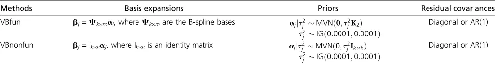
Parameter estimation:Now everything can be put together. In the basic form of the regression model (1), the param-eters bj(tr)(r = 1,. . .,k) are reparameterized by ajh(h = 1,. . .,m) defined in (3) and (4) after the B-spline basis expan-sions, and then we can specify the likelihood function as Table 1 Key features of the functional model and the nonfunctional model
Methods Basis expansions Priors Residual covariances
VBfun bj=Ck·maj, whereCk·mare the B-spline bases ajjt2j MVNð0;t2jK2Þ t2
j IGð0:0001;0:0001Þ
Diagonal or AR(1)
VBnonfun bj= Ik·kaj, where Ik·kis an identity matrix ajjt2j MVNð0;t2jIk·kÞ t2
j IGð0:0001;0:0001Þ
Diagonal or AR(1)
pYja0;a1;. . .;ap;S0
¼ Qn i¼1
MVN yijCa0þ Pp
j¼1
xijCaj;S0 !
; (11)
whereyi= [yi(t1),. . .,yi(tk)]T, anda
j= [aj1,. . .,ajm]T. The hierarchical smoothness priors pðajjs2jÞpðs2jÞ for aj (j = 0,. . .,p) were proposed in the last section. When the residual covariance is assumed to be a diagonal matrix
S0, each diagonal entry s2
r (r = 1,. . .,k) is assigned a flat Jeffreys’ prior as pðs2
rÞ}1=s2r to make pðS0Þ ¼
pðs2
1;. . .;s2kÞ ¼ Qk
r¼1pðs2rÞ. Let u¼ ½a0;a1;. . .;ap;t20; t2
1;. . .;t 2 p;s
2 1;. . .;s
2
kwith K= 2(p + 1) +kcomponents. The posterior distribution can be specified as
pðujYÞ}pðYjuÞpðuÞ
¼pYja0;a1;. . .;ap;s21;. . .;s2k
· Qp j¼0 h
p
ajjt2j
p
t2
j i Qk
r¼1
ps2r
: (12)
A variational Bayes (VB) algorithm based on the meanfield theory (Jaakkola and Jordan 2000; Beal 2003; Bishop 2006) can be used to efficiently evaluate the unknown parameters in the model. Specifically, the above defined intractable pos-terior is approximated by a tractable factorized form,
qðujYÞ ¼ QK l¼1
qðuljYÞ
¼qða0jYÞ⋯q
apjY
qt2 0jY
⋯q
t2
pjY
qs2 1jY
⋯qs2kjY:
(13)
We seek an optimal factorized approximate posterior distri-butionq^ðujYÞby minimizing the Kullback–Leibler divergence KLðqkpÞ ¼RQqðujYÞ ln ðqðujYÞ=pðujYÞÞdu or, equivalently,
maximizing a lower bound of the log-marginal distribution ln
p(Y) defined asLðqðujYÞÞ ¼ RQqðujYÞ ln ðpðu;YÞ=qðujYÞÞdu, whereQrepresents the whole parameter space ofu. It can be shown that such a minimization/maximization is reached at
^
qðuljYÞ}exp n
E^qðu2ljYÞ½ln pðu;YÞ o
; l¼1;. . .;K; (14)
whereE^qðu2ljYÞ½is the posterior expectation with respect to the factorized approximate distribution with thelth compo-nent removed. Since the posterior model belongs to the conjugate exponential family, all the required approximate distributions^qðuljYÞin (14) can be recognized as standard distributions. Then an iterative coordinate descent algo-rithm can be easily used to update ^qðjYÞ in (13) for each parameter based on Equations 14 sequentially until conver-gence. After obtaining the approximate posterior distribution ^
qðajjYÞfor markerj(j= 1,. . .,p), interesting quantities such as posterior mean and posterior covariance matrix are directly available.
When the stationary AR(1) residual covariance is used, the covariance matrix S0 is actually controlled by two parameters, s2
0 andr (0,r,1). We may further assign a noninformative Jeffreys’prior fors2
0 aspðs20Þ}1=s20 and a uniform prior for rasp(r) = 1[0,1]. A factorized form of
the approximate posterior distribution similar to that in Equation 13 can be specified, and the marginal distributions
q(|Y) for all the parameters except r can be optimized based on Equation 14 as above. The parameter r is not conjugate in the posterior and it is difficult to incorporate into the above-mentioned VB updating procedure. To han-dle this, we can apply the idea offixed-form VB approxima-tion (Salimans and Knowles 2013), by preassumingq(r|Y)
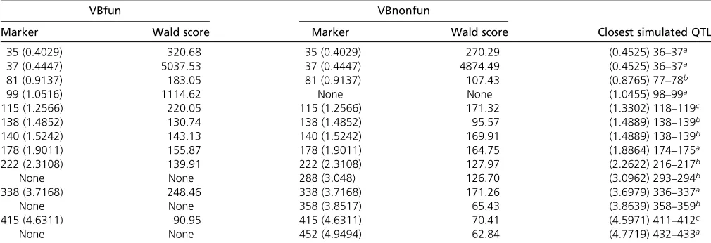
to be a Beta(r|m1, m2) distribution with unknown shape parametersm1andm2. The parametersm1andm2, controlling Table 2 The results of QTLMAS2009 data analysis, including the selected markers, their locations (in brackets), the corresponding Wald scores, and the closest true simulated QTL
VBfun VBnonfun
Marker Wald score Marker Wald score Closest simulated QTL
35 (0.4029) 320.68 35 (0.4029) 270.29 (0.4525) 36–37a
37 (0.4447) 5037.53 37 (0.4447) 4874.49 (0.4525) 36–37a
81 (0.9137) 183.05 81 (0.9137) 107.43 (0.8765) 77–78b
99 (1.0516) 1114.62 None None (1.0455) 98–99a
115 (1.2566) 220.05 115 (1.2566) 171.32 (1.3302) 118–119c
138 (1.4852) 130.74 138 (1.4852) 95.57 (1.4889) 138–139b
140 (1.5242) 143.13 140 (1.5242) 169.91 (1.4889) 138–139b
178 (1.9011) 155.87 178 (1.9011) 164.75 (1.8864) 174–175a
222 (2.3108) 139.91 222 (2.3108) 127.97 (2.2622) 216–217b
None None 288 (3.048) 126.70 (3.0962) 293–294b
338 (3.7168) 248.46 338 (3.7168) 171.26 (3.6979) 336–337a
None None 358 (3.8517) 65.43 (3.8639) 358–359b
415 (4.6311) 90.95 415 (4.6311) 70.41 (4.5971) 411–412c
None None 452 (4.9494) 62.84 (4.7719) 432–433a
For the Wald tests, the critical value corresponding to the significance level 0.05 is 18.31 for the estimates of VBfun (chi-square distribution with 10 d.f.) and 11.07 for the estimates of VBnonfun (with 5 d.f.), respectively (assuming the diagonal covariance structure in the model).
aSimulated QTL effects onf
1of the simulated logistic growth curves (traits), respectively. bSimulated QTL effects onf
3of the simulated logistic growth curves (traits), respectively. cSimulated QTL effects onf
the shape of the approximate marginal posterior distribution, can be estimated by using the novel Monte Carlo sampling-based method introduced in Salimans and Knowles (2013). Details of these VB algorithms are presented inAppendix B.
Variable selection:In principle, it is possible to execute the VB algorithm on the multivariate posterior model with a whole set of markers included and then construct the Wald test statistic based on the posterior mean and co-variance estimate ofajfor thejth marker (seeAppendix A) to detect QTL. A similar strategy has been used in some MCMC-based functional mapping studies (Xing et al.
2012). However, it has been shown that although the VB can generally provide accurate posterior mean estimates for the parameters, posterior uncertainties (e.g., posterior var-iances) are often underestimated (Grimmer 2011; Li and Sillanpää 2012), compared with MCMC. Therefore, the Wald test statistic constructed based on a VB estimate may not be reliable for screening the true positive signals, which motivates us to seek an alternative way to detect QTL un-der the VB scheme. However, we can nevertheless compute the Wald statistic for each marker and consider them as scores for ranking the markers. Specifically, if we consider a model denoted as M with only a subset of markers in-cluded, the corresponding marginal distributionp(Y|M) is called the model evidence or marginal likelihood. The parameter vector in the model M can be defined as
uM ¼ ½a0;aj;j2M;t20;tj2;j2M;s21;. . .;s2r. With the mar-ginal likelihoods for all the models computed, we may go
in two directions: (i) calculate the posterior distribution
p(M|Y)}p(Y|M)p(M) of different models given the data to find which model is preferable [if the prior p(M) is uniform, thenp(M|Y)}p(Y|M) (Bishop 2006)], and (ii) compare two models M1 and M2 by the Bayes factor BF¼pðYjM1Þ=pðYjM2Þ (Kass and Raftery 1995). Al-though the marginal likelihood p(Y|M) cannot be analytically computed for our problem, in variational Bayes estimation, the above-mentioned lower bound
Lð^qðuMjY;MÞÞ ¼ R
QMq^ðuMjY;MÞlnðpðuM;YjMÞ=^qðuMjY;MÞÞ duMcan be treated as an approximation (Bishop 2006). We assume that the prior p(M) is uniformly distributed, and then we can choose an optimal model (the best subset of markers) by satisfying M^ ¼arg maxMLð^qðuMjY;MÞÞ (Beal and Ghahramani 2003). Since it is impractical to perform the VB and compute the lower bounds for all possible com-binations of markers, we use a matching pursuit-like greedy algorithm, which is adapted here from Nott et al. (2012), who considered a different model structure. This procedure produces a sequence of candidate models, and we choose the one corresponding to the largest value of the lower bound. Since usually we are interested only in a small num-ber of QTL with large effects, we could stop the algorithm at an early stage by selecting only a small number of variables into the model without considering the whole solution path. In this case, the algorithm will search only through the low-dimensional space, which can be implemented very efficiently. Further details of this algorithm are shown inAppendix C.
Example Analyses
We evaluate performance of our methods with both simu-lated and real data examples. Our simulation analyses are largely based on the simulated data from the QTLMAS2009 workshop (Costeret al.2010), and the real data were orig-inally analyzed in Xiong et al. (2011). For parameter esti-mation and variable selection, we implemented both the functional multitrait VB approach and the nonfunctional multitrait VB approach presented in this article on all these data sets. For simplicity, here we name them asVBfunand VBnonfun, respectively. Furthermore, both diagonal and AR (1) structures were considered in each case to model resid-ual covariance. For the remainder, some of the key features of VBfun and VBnonfun are summarized in Table 1. The methods were implemented in MATLAB on a desktop with an Intel Core 2 2.13 GHz processor and 2 Gb memory. In practice, we used the MATLAB codes (publicly available at
http://www.psych.mcgill.ca/misc/fda/software.html) de-veloped by Ramsayet al.(2009) to generate cubic B-spline bases. Our own MATLAB codes for implementing VBfun and VBnonfun methods are available inSupporting Information,
File S1.
Analysis of QTLMAS2009 simulated data
Briefly, the simulated data set includes 453 SNP markers distributed over five chromosomes of 1 M each from 2025 individuals with a certain population structure and the growth traits following logistic curves yðtÞ ¼
f1=ð1þexp ððf22tÞ=f3ÞÞmeasured overfive time points (0, 132, 265, 397, and 530 days). In total, 18 additive QTL were simulated, with 6 contributing to each of the three parameters f1 (asymptotic yield), f2 (inflection point), and f3(slope of the curve) of a growth curve. Both geno-type (with map information) and phenogeno-type data are pub-licly available (Coster et al. 2010). The same data set has been analyzed by an MCMC approach of Heuven and Janss (2010) and Sillanpääet al.(2012). A fundamental difference
in model strategies between their approaches and ours has been explained in the Introduction. To compare with Heuven and Janss (2010), the same subsample of 1000 individuals is used in our simulation analyses.
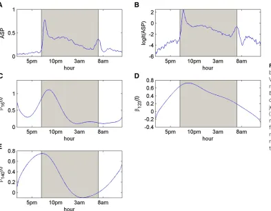
In VBfun, we specified six equidistant knots on the time domain [0, 530]. Note that the number of B-spline bases equals the number of knots plus the spline order, so if the spline order is 4, we obtain 10 B-spline bases in total. For both VBfun and VBnonfun, we ran the VB forward selection for 20 steps that continued with a backward selection procedure (we use the same procedure for the other two data examples). We then identified the best set of variables corresponding to the maximum of the lower bounds. Here we first describe the results by assuming the diagonal residual covariance structure, which might be a more reasonable assumption for the QTLMAS2009 data, since no residual dependence structure was simulated there. The information from the detected QTL is summarized in Table 2. The best model selected by VBfun includes 11 markers, which are all located very close to some of the true simu-lated QTL. The estimated trend functions of the genetic effects for the 11 selected markers are shown in Figure 1. The trend functions have similar shapes to the logistic growth curves. VBnonfun detects 13 markers that are largely overlapping with the markers found by VBfun, in which all the others are located close to some simulated QTL except marker 452. The estimated trend functions from VBnonfun are shown in Figure S1. In total, VBfun and VBnonfun detected 9 and 11 true simulated QTL, respec-tively, which is comparable to the results shown in Heuven and Janss (2010), where they reported 9 correctly detected QTL (with false discovery rate,0.05). Similarly to that in Heuven and Janss (2010), our methods are able to detect most of the QTL controlling the parametersf1andf3of the logistic growth curve, but find fewer that control f2. In addition, Sillanpää et al.(2012) correctly detected 6 QTL (with QTL inclusion probability.0.5) and 8 QTL (with QTL inclusion probability.0.05). Note that they considered only 500 individuals, which may reduce the statistical power to detect QTL with high probability. Compared to the MCMC approaches of Heuven and Janss (2010) and Sillanpääet al.
(2012), one major benefit of our VB method is its computa-tional efficiency. For both VBfun and VBnonfun, the whole computational procedure took only ,1 min, whereas the MCMC methods may take hours.
Additionally, the results by assuming AR(1) residual covariance structure are shown in Table S1, Figure S2, and Figure S3. Here, the analyses took a longer time, be-cause a stochastic optimization step is built into the VB al-gorithm for updating the nonconjugate part of the model. The results of both VBfun and VBnonfun here turned out to be slightly worse than in the case of the diagonal covariance structure, in the sense that fewer numbers of QTL are cor-rectly detected. Amazingly, the mean estimate of the param-eter r, measuring the decline of the correlation with time lag, is 0.91. This indicates that the temporal correlation Table 3 The simulated trend functions for the intercept and
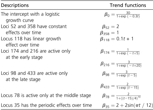
nine QTL
Descriptions Trend functions
The intercept with a logistic growth curve
b0¼1þexp 30ð20:3tÞ
Loci 52 and 358 have constant effects over time
b52¼2 b358¼1 Locus 118 has linear growth
effect over time
b118¼0.1t+ 1
Loci 174 and 216 are active only at the early stage
b174¼1þexp 1ð2tþ5Þ
b216¼1þexp ð32tþ20Þ
Loci 98 and 433 are active only at the late stage
b98¼1þexp3 ðt25Þ
b433¼1þexp 2ðt215Þ
Locus 78 is active only at the middle stage b78¼1þððt2215Þ=4Þ10
among the (non-QTL) residual errors is extremely high, al-though no such residual dependencies were actually simu-lated. Note that the QTL effects were simulated to the latent trait variables f1,f2, andf3, so that they only indirectly influenced the characteristic of the real phenotypes. Their way of simulation might accidently introduce the high re-sidual correlation to the phenotype data, and the methods assuming AR(1) residual covariance may have difficulties in associating observed dependency into the correct origin. However, the detected QTL between two residual structures partially coincide.
More complicated simulation studies
Here on the basis of the genotype data with 453 markers and 1000 individuals from the QTLMAS2009 workshop, we simulated new phenotype data by having nine additive QTL at markers 35, 52, 78, 98, 118, 174, 216, 358, and 433 together with an intercept term in the simulation model. The trend functions of the genetic and nongenetic effects simulated within the time domain [0, 24] (hr) are given in Table 3. Generally, they were simulated as different curves (linear, logistic, sine . . .) with various degrees of smooth-ness. All the other 444 markers were assumed to be inactive over time. The k simulated time points are equally spaced from 0 to 24. The residual termsei(tr) (r= 1,. . .,k) were simulated from the AR(1) process. The dynamic phenotype data were then generated based on Equation 1.
Again, VBfun and VBnonfun were compared using either diagonal residual covariance structure or AR(1) structure.
Evaluation of parameter estimation:Wefirst evaluate how accurately our methods can estimate the trend functions of the intercept and the genetic effects without any variable selection. We simulated four data sets with all possible combinations of k= 10, 100 (number of time points) and r = 0.5, 0.8 (residual correlation). The noise levels2
0 was fixed to be 15. The average heritabilities over time points
varied from 0.09 to 0.23 for those four data sets. We used both VBfun and VBnonfun with the assumption of AR(1) residual covariance structure to estimate the effects of nine simulated QTL. In VBfun, we specified 16 and 46 equidistant knots (corresponding to 20 and 50 B-spline bases) whenk= 10 andk= 100, respectively. Based on our experiments, the results were not sensitive to the number of knots we chose if the number was set to be large enough. However, it is not recommended to use too large a number of knots to save computation time. To measure the accuracy of the parame-ter estimates, we calculated the mean squared error (MSE) for each simulated QTL (including the intercept term) as
MSEbj¼1 k
b^j2bj2 2
¼1 k
Ca^j2bj 2
2
; (15)
where bjis the simulated trend function for markerj, and
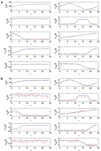
Ca^jis the estimated trend function. The results are summa-rized in Table 4. Also see Figure 2 including a comparison between the estimated trends and the true simulated trends for the case of k= 100 andr= 0.5. Results for the other three cases are presented inFigure S4,Figure S5, andFigure S6. For all the data sets, the posterior mean estimates of the parametersr and s2
0 are not far from their true simulated values, indicating the good performance of the fixed-form VB estimation. Regarding the QTL effects, VBfun tends to provide more accurate estimates than VBnonfun. Taking the case ofk= 100 andr= 0.5 as an example (see Figure 2), the trend functions estimated by VBfun are almost identical to the true simulated trends. Whereas VBnonfun mistakenly shrinks the estimated effects (over time) of marker 174 to-ward zero, the estimates of other markers show highly os-cillating patterns. VBfun seems to perform best when the number of time points is large (i.e.,k = 100) and the re-sidual correlation is not high (i.e.,r= 0.5).
If the diagonal residual covariance structure is assumed in the model (results are shown in Table S2, Figure S7, Table 4 The mean squared error comparing the estimated trend functions to the simulated ones
k= 10 k= 10 k= 100 k= 100
u= 0.5 k= 0.8 u= 0.5 u= 0.8
h2= 0.2265 h2= 0.0922 h2= 0.2347 h2= 0.1259
QLT effects F N F N F N F N
b0 0.2194 2.0375 0.4933 14.5590 0.0246 1.7757 0.1166 19.4684
b35 0.0704 0.1483 0.1138 0.5161 0.0189 0.1267 0.0573 0.5326
b52 0.2535 0.7231 0.0616 3.9968 0.0247 0.2045 0.0324 3.9995
b78 0.0921 0.1037 0.0937 0.1542 0.0248 0.1185 0.1442 1.2072
b98 0.1505 0.0725 0.4961 0.5038 0.0160 0.2116 0.4147 1.5341
b118 0.0127 0.0239 0.1416 0.1495 0.0063 0.0695 0.0185 0.1778
b174 0.0513 0.7201 0.1866 0.7229 0.0129 0.7464 0.1099 0.7473
b216 0.0459 0.0586 0.2224 0.0369 0.0099 0.0606 0.0677 1.1692
b358 0.0069 0.0493 0.0385 0.9960 0.0022 0.0481 0.0085 0.9988
b433 0.2278 0.0278 0.2753 2.2965 0.0332 0.1145 0.3022 2.3295
E½s2
0 14.8034 14.7677 14.9339 14.9758 14.9081 14.9560 15.0325 15.1299
E[r] 0.5088 0.5138 0.7796 0.7882 0.4987 0.5036 0.7779 0.7876
Figure S8,Figure S9, andFigure S10), VBfun seems to pro-vide identical estimates compared to the case when AR(1) structure is assumed. On the other hand, VBnonfun per-forms better together with diagonal covariance structure than with AR(1), in the sense that it does not mistakenly shrink the effects of any QTL toward zero.
s2
0 and correlation levelr werefixed to be 10 and 0.5, re-spectively. These simulations were repeated 50 times. We then applied the proposed VB methods assuming the AR (1) residual covariance structure on the data and monitored how many times each QTL was correctly identified by VBfun and VBnonfun in each of the four simulated conditions. The results are presented in Table 5. Overall, the VBfun method consistently performed better than VBnonfun. Especially when the number of individuals is small and the number of time points is large (i.e.,n= 200 andk= 100), VBfun tends to correctly detect eight of nine QTL with very high frequency, but VBnonfun detected none of them. Whenn= 500 andk= 100, VBfun is able to correctly identify all nine QTL in almost all 50 replicates, while VBnonfun detects only three. However, when n = 200 and k = 10, VBfun and VBnonfun behave similarly by selecting only two QTL frequently.
The results of both methods assuming the diagonal residual covariance structure are presented in Table S3. VBfun assuming the residual diagonal covariance structure identifies the correct set of QTL equally as well as the method together with the AR(1) residual covariance, but assuming the diagonal residual covariance results in more false positive QTL. On the other hand, VBnonfun assuming the residual diagonal covariance seems to correctly detect more true QTL than assuming AR(1) covariance.
To further evaluate how well our proposed methods can avoid false positive signals, we simulated another four replicated null data sets, where only an intercept term but no QTL influenced the phenotypes. The sample sizes, number of time points, and residual covariance structures were simulated as above. Results of the average number of false positive QTL over 50 replicates are shown in Table 6. We found that only VBfun together with the diagonal co-variance structure may tend to produce a few false positives in some of the replicates, when the nontrivial temporal re-sidual covariance structure indeed exists.
Analysis of mouse behavioral data
In the real data analysis, we considered a mouse behavioral data set, which has been previously analyzed by Xionget al.
(2011) and is publicly available at QTL Archive (http:// qtlarchive.org/db/q?pg=projdetails&proj=xiong_2011). The phenotype data contain active state probabilities (ASP) (y2[0, 1]) with 222 repeated measurements at each con-secutive 6-min time interval within 24 hr (from 1:48PM to 1:54 PM to 11:54AM to12:00AM, with 7PM to 7AM as the dark period and otherwise as the light period) for 89 back-cross mice. The genotype data consist of 233 informative polymorphic SNP markers distributed over 19 chromo-somes. Note that the data are quite challenging from the analysis point of view mainly due to the fact that (1) both the numbers of markers and time points are larger than the number of individuals and (2) considerable variations were shown among the active-state probabilities of the mice (Xiong et al. 2011), and the shape of the mean trajectory (see Figure 3A) is also quite complex. For detailed informa-tion on phenotyping and genotyping, please refer to Gould-ing et al. (2008) and Xiong et al. (2011). Before the statistical analysis, we performed the following three pre-processing steps:
1. The missing genotypes were replaced by their conditional expectations estimated from theirflanking markers with known genotypes (Haley and Knott 1992) once before the analysis.
2. We performed the logit transformation lnðy=ð12yÞÞ to the phenotypic measurements (Warton and Hui 2011), so that their values were not restricted to the domain [0, 1]. Specially, for those measurements with ASP of 0 and 1, we first changed values to 0.001 and 0.999, respectively, and then performed logit transformation. The mean trajectories of original and transformed phe-notypic data are shown in Figure 3, A and B, respectively. Although the logit transformation did not reduce any complexity in the original data, we found that, by directly applying our VB approaches to the original percentage phenotypes without any transformation, the methods would produce some unreasonable results [i.e., the esti-mated lower boundLð^qðuMjY;MÞÞgave positive values]. 3. To generate B-spline bases, we discretized the 222 time inter-vals by a set of single time points [1.9, 2,. . ., 23.9, 24] (e.g., 1.9 represents 1:48PM, and 24 represents 12:00AM). Table 5 The number of times each QTL has been correctly selected
over 50 replications, together with the average number of wrongly selected markers (false positives)
n= 200 n= 200 n= 500 n= 500
k= 10 k= 100 k= 10 k= 100
QTL F N F N F N F N
35 50 47 50 0 50 50 50 50
52 4 0 49 0 44 0 50 0
78 0 0 50 0 37 3 50 0
98 0 0 45 0 36 0 50 0
118 49 43 50 0 50 50 50 50
174 0 0 11 0 2 0 46 0
216 19 1 49 0 47 38 50 0
358 4 0 50 0 43 0 50 0
433 0 0 43 0 27 0 50 0
Average false positive 0.04 0.04 0.32 0 0.06 0.07 0.08 0
F and N represent VBfun and VBnonfun, respectively [assuming the AR(1) covariance structure in the model].
Table 6 Simulation study under the null: the average number of wrongly selected markers (false positives) over 50 replications
n= 200 n= 200 n= 500 n= 500
k= 10 k= 100 k= 10 k= 100
QTL F N F N F N F N
Diagonal 0.08 0 0.38 0 0.08 0 0.40 0
AR(1) 0 0 0 0 0 0 0 0
Here wefirst describe the results of VBfun when the AR (1) residual covariance structure is assumed. As in the last simulated example, we generated 50 B-spline bases needed in VBfun as an upper limit for complexity. VBfun then suggested the best model with three putative QTL, whose positions are shown in Table 7. The posterior mean esti-mates of AR(1) parameters s2
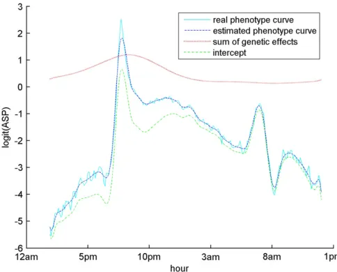
0 and r are 1.79 and 0.66, respectively. Among these three putative QTL, loci 16 (rs3689947) and 123 (rs6207781), with the largest Wald scores, are located at 81.40 cM on chromosome 1 and at 20.74 cM on chromosome 9, respectively. The estimating equations approach of Xionget al.(2011) detected two ma-jor QTL, which are located at 75 cM (between loci 15 and 16) on chromosome 1 and at 10 cM (at locus 119) on chromosome 9 [S. Sen (University of California, San Fran-cisco), personal communication]. Note that in the ge-notype data some adjacent markers are very highly correlated with each other, and our greedy search algo-rithm tends to select only a single marker from a group of highly correlated markers. This might explain why the positions found by our method are slightly different from theirs. In addition, our method detected another interest-ing locus 140, on chromosome 10. An overall genetic effect trend of the three putative QTL is calculated by(P89i¼1ððxi16CE½a16þxi123CE½a123þxi140CE½a140Þ=89Þ), and the curve is shown in Figure 4. The overall trend of the genetic effects shows a peak between 5AMand 2PM, during which time the mean trajectory of the phenotypes also shows a clear peak. This indicates that the three putative QTL
detected by our method may contribute to the phenotypic variation during the time period when the mice are highly activated. We may further reestimate the phenotypes by summing the estimated intercept and genetic effects of the selected loci. The mean trajectory of the reestimated pheno-types is also shown in Figure 4, which provides a smooth description of the original mean phenotype curve.
On the other hand, when the diagonal covariance struc-ture is assumed (results are shown inTable S4,Figure S11, andFigure S12), VBfun is able to detect loci 18, 123, and 137 (note that loci 18 and 137 are near to loci 16 and 140), which were also found in the AR(1) case. However, additionally, VBfun tends tofind many other markers with relatively small effects that are false positives. Thus, we can conclude that assuming a time-dependent AR(1) residual covariance seems to effectively control false positive signals.
Finally, VBnonfun and two different residual covariance structures were applied on the mouse data as well, but they did not detect any signals (results not shown).
Discussion
without the need to explicitly determine the optimal number of B-spline bases). Our nonparametric method should be generally applicable to many kinds of dynamic traits whether their trajectories are smooth or rather complicated. In this article, we have not considered yet the possible im-pact of some environmental covariates such as temperature and age variables and their interactions with QTL, as well as the QTL–QTL interactions on the target dynamic traits. Fol-lowing works such as Zhang and Xu (2005), Yi and Banerjee (2009), Minet al. (2011), and Li and Sillanpää (2012), it is not difficult to extend our current marker set by includ-ing the environmental covariates or the pairwise marker– environment or pairwise marker–marker interaction terms as new“marker”variables for variable selection.
Our model specification is largely based on the Bayesian P-splines, which has been applied in various nonparametric modelingfields such as structured additive models (Fahrmeir
et al. 2010) and time-varying coefficient models (Lee and Shaddick 2007). One common problem of such a model specification is that a relatively large number of B-spline bases need to be used in the model, which makes the sim-ulation-based MCMC algorithm infeasible for large-scale data sets with hundreds of markers and time points. This motivates us to alternatively use a fast deterministic vari-ational Bayes algorithm for computation. The VB approxi-mation method can not only provide accurate posterior mean estimates to the parameters of genetic effects, but also provides a lower bound estimate of the model evi-dence that can be used to guide variable selection (Beal and Ghahramani 2003). The matching pursuit-like algo-rithm adapted here from Nott et al. (2012) is a simple and efficient method for searching an“optimal subset”of markers that roughly maximizes lower bounds. However, since such a greedy algorithm does not fully explore the whole model space, it usually cannotfind a“perfect model ” that corresponds to the global maximum of the lower bounds especially in the case of polygenic traits. We rec-ommend using such a procedure only in the case of sparse genetic architecture to seek a small number of markers with relatively large genetic effects.
An important goal of our data analyses was to com-pare the functional (multivariate) mapping approach (i.e., VBfun) and the general nonfunctional multiple-trait ap-proach (i.e., VBnonfun) for analyzing the functional valued dynamic traits. Overall, the results from those three
exam-ples showed that the functional approach performs better than or at least equally as well as the nonfunctional ap-proach, from the perspective of both parameter estimation and variable selection. Especially when the number of time points is relatively large and the number of individuals is relatively small, the functional approach tends to show much higher statistical power to detect QTL than the non-functional approach, indicating that the non-functional approach owns the advantage of combining the information from dif-ferent repeated measurement points by specifying basis expansions and smoothing priors for genetic effects in the model. Dynamic phenotype data measured at a large num-ber of time points are often available from some high-throughput automated phenotyping platforms (e.g., Eberius and Lima-Guerra 2009). On the other hand, when the num-ber of time points is small, the benefit of using the functional approach is reduced. Note that our VB framework is quite flexible in the sense that the B-splines can be substituted by many other possible methods of basis expansions and corre-sponding priors as well. In practice, it is useful to compare different methods and choose the most preferable one.
The primary aim of our nonparametric method is to determine a subset of important markers approximating QTL and estimate the trends of their genetic effects over time. We also tested two possible residual covariance structures, (i) a nonstationary diagonal covariance structure and (ii) a station-ary AR(1) covariance structure, and evaluated their impacts on the QTL mapping. In most of our analyses, we found that compared to the AR(1) covariance structure, the simple diagonal structure assuming time independence of residual errors does not significantly affect the accuracy of the parameter estimation, but tends to significantly underestimate the Table 7 The results of mouse behavioral data analysis by using
VBfun, which assumed the AR(1) residual covariance structure, including the selected markers, their chromosomes, locations, and the corresponding Wald scores
Marker Chromosome Location (cM) Wald score
16 (rs13476259) 1 81.40 148.6427
123 (rs6207781) 9 20.74 122.1237
140 (rs3654717) 10 55.93 110.5854
For the Wald tests, the critical value corresponding to the significance level 0.05 is 67.50 for the estimates (chi-square distribution with 50 d.f.).
uncertainty (i.e., the posterior covariance for each marker), which may result in including some false positive QTL into the variable selection procedure. Therefore, even though the computation with AR(1) covariance structure is more expen-sive due to the presence of nonconjugacy in the posterior, it might be a more suitable choice especially when the herit-abilities of the dynamic traits under study are low. Other more complicated covariance structures such as some stationary parametric structures (Liu and Wu 2009) or non-parametric structures (Yap et al. 2009) can be possibly incorporated if needed, but they require the development of more specific algorithms for the computation of those newly involved parameters. Furthermore, it is necessary to point out that due to the approximative nature of the VB algorithm, the uncertainty estimates for markers may still be underestimated even by using an appropriate residual co-variance structure or, by other means, the estimated Wald statistic might be upward biased. On the other hand, the MCMC method is able to provide more accurate uncertainty estimates than the VB methods. Thus, after obtaining a small subset of markers from our VB variable selection procedure, we may then apply a MCMC algorithm to more accurately estimate the Wald statistics and perform the formal hypoth-esis testing. These can be taken as topics for future research.
Acknowledgments
We are grateful to the three anonymous referees for their valuable comments, which helped us to substantially im-prove the contents of this article. This work was supported by the Finnish Graduate School of Population Genetics and by a research grant from the Academy of Finland.
Literature Cited
Banerjee, S., B. S. Yandell, and N. Yi, 2008 Bayesian QTL map-ping for multiple traits. Genetics 179: 2275–2289.
Beal, M. J., 2003 Variational algorithms for approximate Bayesian inference. Ph.D. Thesis, University of London, London. Beal, M. J., and Z. Ghahramani, 2003 The variational Bayesian
EM algorithm for incomplete data: with application to scoring graphical model structures. Bayesian Stat. 7: 453–464. Bishop, C. M., 2006 Pattern Recognition and Machine Learning.
Springer-Verlag, New York.
Carbonetto, P., and M. Stephens, 2012 Scalable variational infer-ence for Bayesian variable selection in regression, and its accu-racy in genetic association studies. Bayesian Anal. 7: 73–108. Chib, S., and I. Jeliazkov, 2008 Inference in semiparametric
dy-namic models for binary longitudinal data. J. Am. Stat. Assoc. 101: 685–700.
Coster, A., J. W. M. Bastiaansen, M. P. L. Calus, C. Maliepaard, and M. C. A. M. Bink, 2010 QTLMAS 2009: simulated dataset. BMC Proc. 4: S1.
de Boor, C. M., 2001 A Practical Guide to Splines. Springer-Verlag, New York.
Eberius, M., and J. Lima-Guerra, 2009 High-throughput plant phenotyping: data acquisition, transformation, and analysis, pp. 259–278 inBioinformatics, edited by D. Edwards, J. Stajich, and D. Hansen. Springer-Verlag, New York.
Eilers, P. H. C., and B. D. Marx, 1996 Flexible smoothing using B-splines and penalized likelihood. Stat. Sci. 11: 89–121. Fahrmeir, L., and T. Kneib, 2011 Bayesian Smoothing and
Regres-sion for Longitudinal, Spatial and Event History Data. Oxford University Press, New York.
Fahrmeir, L., T. Kneib, and S. Konrath, 2010 Bayesian regularisa-tion in structured additive regression: a unifying perspective on shrinkage, smoothing and predictor selection. Stat. Comput. 20: 203–219.
Gee, C., J. L. Morrison, D. C. Thomas, and W. J. Gauderman, 2003 Segregation and linkage analysis for longitudinal meas-urements of a quantitative trait. BMC Genet. 4: S21.
Gong, Y., and F. Zou, 2012 Varying coefficient models for map-ping quantitative trait loci using recombinant inbred inter-crosses. Genetics 190: 475–486.
Goulding, E. H., A. K. Schenk, P. Juneja, A. W. MacKay, J. M. Wade et al., 2008 A robust automated system elucidates mouse home cage behavioral structure. Proc. Natl. Acad. Sci. USA 105: 20575–20582.
Grimmer, J., 2011 An introduction to Bayesian inference via var-iational approximations. Polit. Anal. 19: 32–47.
Haley, C. S., and S. A. Knott, 1992 A simple regression method for mapping quantitative trait loci in line crosses using flanking markers. Heredity 69: 315–324.
Hastie, T., R. Tibshirani, and J. Friedman, 2009 Elements of Sta-tistical Learning, Ed. 2. Springer-Verlag, New York.
Heuven, H. C. M., and L. L. G. Janss, 2010 Bayesian multi-QTL mapping for growth curve parameters. BMC Proc. 4: S12. Hurtado, P. X., S. K. Schnabel, A. Zaban, M. Veteläinen, E. Virtanen
et al., 2012 Dynamics of senescence-related QTLs in potato. Euphytica 183: 289–302.
Jaakkola, T. S., and M. I. Jordan, 2000 Bayesian parameter esti-mation via variational methods. Stat. Comput. 10: 25–37. Jiang, C., and Z.-B. Zeng, 1995 Multiple trait analysis of genetic
mapping for quantitative trait loci. Genetics 140: 1111–1127. Kass, R. E., and A. E. Raftery, 1995 Bayes factors. J. Am. Stat.
Assoc. 90: 773–795.
Lang, S., and A. Brezger, 2004 Bayesian P-splines. J. Comput. Graph. Stat. 13: 183–212.
Lee, D., and G. Shaddick, 2007 Time-varying coefficient models for the analysis of air pollution and health outcome data. Bio-metrics 63: 1253–1261.
Li, J., K. Das, G. Fu, R. Li, and R. Wu, 2011 The Bayesian LASSO for genome-wide association studies. Bioinformatics 27: 516–523. Li, J., R. Li, and R. Wu, 2012 Bayesian group lasso for nonparamet-ric varying coefficient models. Available at:http://www.personal. psu.edu/jzl185/jonathan/paper/bayesian_lasso_fi.pdf.
Li, Z., and M. J. Sillanpää, 2012 Estimation of quantitative trait locus effects with epistasis by variational Bayes algorithms. Ge-netics 190: 231–249.
Lin, M., and R. Wu, 2006 A joint model for nonparametric func-tional mapping of longitudinal trajectory and time-to-event. BMC Bioinformatics 7: 138.
Liu, T., and R. Wu, 2009 A Bayesian algorithm for functional mapping of dynamic complex traits. Algorithms 2: 667–691. Logsdon, B. A., G. E. Hoffman, and J. G. Mezey, 2010 A
varia-tional Bayes algorithm for fast and accurate multiple locus ge-nome-wide association analysis. BMC Bioinformatics 11: 58. Ma, C., G. Casella, and R. Wu, 2002 Functional mapping of
quan-titative trait loci underlying the character process: a theoretical framework. Genetics 161: 1751–1762.
Meier, L., and P. Bühlmann, 2007 Smoothingℓ1-penalized estima-tors for high-dimensional time-course data. Electron. J. Stat. 1: 597–615.
Nott, D. J., M. N. Tran, and C. Leng, 2012 Variational approxima-tion for heteroscedastic linear models and matching pursuit al-gorithms. Stat. Comput. 22: 497–512.
Ramsay, J., G. Hooker, and S. Graves, 2009 Functional Data Anal-ysis with R and MATLAB. Springer-Verlag, New York.
Salimans, T., and D. A. Knowles, 2013 Fixed-form variational posterior approximation through stochastic linear regression. Available at:http://arxiv.org/abs/1206.6679.
Segura, V., B. J. Vilhjálmsson, A. Platt, A. Korte, . Seren et al., 2012 An efficient multi-locus mixed-model approach for ge-nome-wide association studies in structured populations. Nat. Genet. 44: 825–830.
Sillanpää, M. J., P. Pikkuhookana, S. Abrahamsson, T. Knürr, A. Frieset al., 2012 Simultaneous estimation of multiple quanti-tative trait loci and growth curve parameters through hierarchi-cal Bayesian modeling. Heredity 108: 134–146.
Warton, D. I., and F. K. C. Hui, 2011 The arcsine is asinine: the analysis of proportions in ecology. Ecology 92: 3–10.
Wu, R., and M. Lin, 2006 Functional mapping-how to map and study the genetic architecture of dynamical complex traits. Nat. Rev. Genet. 7: 229–237.
Xing, J., J. Li, R. Yang, X. Zhou, and S. Xu, 2012 Bayesian B-spline mapping for dynamic quantitative traits. Genet. Res. 94: 85–95.
Xiong, H., E. H. Goulding, E. J. Carlson, L. H. Tecott, C. E. McCul-lochet al., 2011 Aflexible estimating equations approach for mapping function valued traits. Genetics 189: 305–316. Xu, S., 2003 Estimating polygenic effects using markers of the
entire genome. Genetics 163: 789–801.
Yang, J., R. Wu, and G. Casella, 2009 Nonparametric functional mapping of quantitative trait loci. Biometrics 65: 30–39. Yang, R., and S. Xu, 2007 Bayesian shrinkage analysis of
quanti-tative trait loci for dynamic traits. Genetics 176: 1169–1185. Yang, R., J. Li, X. Wang, and X. Zhou, 2011 Bayesian functional
map-ping of dynamic quantitative traits. Theor. Appl. Genet. 123: 483–492. Yap, J. S., J. Fan, and R. Wu, 2009 Nonparametric modeling of longitudinal covariance structure in functional mapping of quantitative trait loci. Biometrics 65: 1068–1077.
Yi, N., and S. Banerjee, 2009 Hierarchical generalized linear models for multiple quantitative trait locus mapping. Genetics 181: 1101–1113. Zhang, Y.-M., and S. Xu, 2005 A penalized maximum likelihood method for estimating epistatic effects of QTL. Heredity 95: 96–104. Zhao, W., H. Li, W. Hou, and R. Wu, 2007 Wavelet-based para-metric functional mapping of developmental trajectories with high-dimensional data. Genetics 176: 1879–1892.
Communicating editor: N. Yi
Appendix A
Our modeling strategy is largely based on an idea of a combination of B-splines with a difference penalty added on the parametersajhdefined in Equation 3 or so called P-splines (Eilers and Marx 1996). An important property of B-splines is that if all the parameters are the same, then thefitted curve is a horizontal line (a constant value). Inspired by this fact, the frequentist P-splines with thefirst- and second-order penalties are defined as
Xm
h¼1
cjhðtÞajhþlj Xm
h¼2
ajh2ajh21 2
(A1)
and
Xm
h¼1
cjhðtÞajhþlj Xm
h¼3
ajh22ajh21þajh222; (A2)
respectively, where lj.0 is a tuning parameter. The difference penalties lj Pm
h¼2ðajh2ajh21Þ 2
or ljPmh¼3ðajh22ajh21þajh22Þ
2
play a role to push the adjacent parameters of B-splines to share similar values to induce the smoothness to the curve. The tuning parameterlj.0 for markerjdetermines how smooth a curve will be. Note that the higher-order penalties can be specified as well, but only thefirst-order and second-order penalties are widely used in practice (Fahrmeir and Kneib 2011). From the perspective of the Bayesian statistics, the difference penalties above can be interpreted as the random walk smoothing priors (Lang and Brezger 2004), which have been introduced previously in Equations 5–9. Next, we explain briefly how to convert the random walk smoothing priors (5)–(9) to the matrix form, which is defined in (10). For the first-order case, from (5) and (7), we can obtainpðajÞ}exp ð2ðð10001 a2j1þ
Pm
h¼2ðajh2ajh21Þ2Þ=t2jÞÞ. It is not difficult to show that
1 1000a
2 j1þ
Xm
h¼2
ajh2ajh21 2
¼aT jU1ajþ
D1aj
T
D1aj; (A3)
where
U1m·m¼
0 B B @
1
1000 0 ⋯ 0
0 0 ⋮
⋮ ⋱ ⋮
0 ⋯ ⋯ 0
1 C C
A and Dð1m21Þ·m¼ 0 B B @
21 1 0
21 1
⋱ ⋱
0 21 1
Then we have ajjt2j MVNð0;t2jK211Þ with K1¼U1þD
T
1D1. Similarly for the second-order case, we obtain
ajjt2j MVNð0;tj2K221Þwith K2¼U2þD
T
2D2, where
U2m·m¼
0 B B B B @
1
1000 0 ⋯ ⋯ 0
0 10001 ⋮
⋮ 0 ⋮
⋮ ⋱ 0
0 ⋯ ⋯ ⋯ 0
1 C C C C
A and D
ðm22Þ·m
2 ¼
0 B B @
1 22 1 0
1 22 1
⋱ ⋱ ⋱
0 1 22 1
1 C C A
Finally, note that, in the original article on Bayesian P-splines (Lang and Brezger 2004), the prior specifications in (5) or (7) and (8) were replaced byp(aj1)}1 orp(aj1)}1 andp(aj2)}1, which results in a rank deficient penalty matrixK1orK2. Our prior setting given above, proposed by Chib and Jeliazkov (2008), guaranteesK1orK2to be full rank, which is required to proceed to the variational Bayes estimation that is introduced inAppendixes BandC.
Appendix B VB Estimation
As mentioned earlier, the meanfield variational Bayes algorithm can be applied to compute a factorized approximate posterior distribution qðujYÞ ¼QKl¼1qðul jYÞ, by minimizing the Kullback–Leibler divergence between it and the true posterior distribution. It is known that the minimization of the KL divergence with respect to eachq(ul|Y) is reached at ^
qðuljYÞ, defined by formula (14). If the posterior belongs to the conjugate exponential family so that^qðuljYÞ for l= 1,. . .,Kcan be derived as standard parametric distributions, then a simple coordinate descent algorithm can be used for sequentially updating each^qðul jYÞ. However, if for one parameterul 9, the marginal distribution^qðul 9jYÞdefined by (14) is
not recognized as any standard distribution, then proceeding with the VB algorithm based on (14) is no longer straightforward, since it might not be possible to derive an analytical form of the expectationE^qðul9jYÞ½ln pðu;YÞ. Instead, we may assume that the marginal approximate distribution oful9is in afixed formqhðul 9jYÞ ¼hðul9Þ exp ðtðul9Þh2aðhÞÞ belonging to the exponential family, where his au·1 vector of natural parameters that determines the shape of the approximate distribution,tðul9Þis a 1·uvector of statistics,a(h) defines the normalizing constant, andhðul9Þis a base
measure. The minimization of the above-mentioned KL divergence with respect to qhðul 9jYÞ is now equivalent to the
optimization problem
^
h¼arg min
h Eqhðul9jYÞ
h
ln qhul 9jY
2Eqhðu2l9jYÞ½ln pðu;YÞ i
; (B1)
where the expectationEqhðu2l9jYÞ½ln pðu;YÞcan be easily computed, if^qðjYÞdefined in (14) for all other parameters expectul9 are standard parametric distributions.
Salimans and Knowles (2013) demonstrated that the minimization is given at
~
h¼Eq^hðul9jYÞ
h
~tul9ÞT~tðul9Þ
i21
Eqhðul9jYÞ h
~tul9ÞTEqh^ðu2l9jYÞ½ln pðu;YÞ i
; (B2)
where h~¼ ½2aðhÞ;h^TT, and~tðul9Þ ¼ ½1;tðul9Þ. If we can sample fromqh^ðul 9jYÞ, then the two expectations in (B2) can be evaluated by the Monte Carlo simulation methods. Based on these ideas, Salimans and Knowles (2013) designed a stochastic optimization algorithm to estimateh^ or, alternatively, an optimal marginal approximate distribution^qðul 9jYÞ ¼qh^ðul 9jYÞ. We use
Algorithm 1 in their article for evaluating the approximate distribution of r, which is a key parameter defining the AR(1) covariance matrix.
Next, following the above principles, we present the specific VB algorithms for estimating the marker effects. The variable selection part is then explained inAppendix C.
ln pðu;YÞ ¼ln 8 < :p
Yja0;a1;. . .;ap;s21;. . .;s2k Yp
j¼0 h
pajjt2j
pt2ji Y
k
r¼1
ps2r
9 = ;
¼ 21 2
Xn
i¼1 2
4k ln 2pþX k
r¼1 ln s2rþ
0
@yi2Ca02Xp j¼1
xijCaj 1 A T
S21 0
0
@yi2Ca02Xp j¼1
xijCaj 1 A 3 5 21 2 Xp
j¼0 h
m ln 2pþm ln t2j þlnjKdj þt2j 2aTjK2d1aj i
þX
p
j¼0 h
a ln b2ln GðaÞ2ðaþ1Þln t2j 2bt2j 2i
2X
k
r¼1
ln ps2k; (B3)
wherea=b= 0.0001. By using formula (14), we can derive the analytical form ofq(•|Y) for each parameter inuas follows. I. Derivation of^qða0jYÞ
By keeping only terms containinga0, we obtain
ln ^qða0 j YÞ}E^qðu=a0jYÞ½ln pðu;YÞ ¼ 2
1 2aT0CT
nCTE½S21 0 CþE
t22
0
KdCa0þP
n
i¼1
yi2P
p
j¼1
xijCE½aj !T
E½S201Ca0þC;
(B4) where C represents those terms that do not contain a0, and E½S021 represents a k · k diagonal matrix with
E½S201 ðr;rÞ ¼E½s22 r
for r= 1,. . .,k. Here the notationE[•] represents the posterior expectation (first moment) of the parameter • with respect to its approximate marginal distribution q^ð•jYÞ. We can recognize from (B4) that ^qða0jYÞ is amultivariate normal distributionwith mean
E½a0 ¼COV½a0CTE½S201 Xn
i¼1 0
@yi2Xp j¼1
xijCE
aj 1A
(B5)
and covariance matrix
COV½a0 ¼
nCTES21 0
CþE½t202Kd21: (B6)
Furthermore, the second moment can be calculated asE½a0aT0 ¼E½a0E½a0TþCOV½a0. II. Derivation of^qðajjYÞ(j = 1,. . ., p)
ln ^qajjY
}E^qðu=ajjYÞ½ln pðu;YÞ ¼ 2 1 2aTjCT
Pn
i¼1
x2
ijCTE½S2 1 0 CþE
h t22
j i
Kd
Caj (B7)
þX
n
i¼1 0
@yi2CE½a02Xp l6¼j
xilCE½al 1 A T
xijE½S201CajþC: (B8)
We recognize ^qða0jYÞas a multivariate normal distribution with mean (or thefirst moment)
Eaj
¼COVaj
CT
E½S201 Xn
i¼1 0
@yi2CE½a02Xp l6¼j
xilCE½al 1
Axij (B9)
and covariance matrix
COVaj
¼ X
n
i¼1
xij2CTE
S21 0
CþE
t22
j
Kd !21
: (B10)
Furthermore, the second moment can be calculated asEajaTj
¼Eaj
Eaj T
þCOVaj
III. Derivation of^qðt2
jjYÞ(j = 1,. . ., p) We have
ln ^q
t2
jjY
}E^qðu=t2
jjYÞ½ln pðu;YÞ ¼ 2
A1jþ1
ln t2 j 2
B1j t2
j þ
C; (B11)
where
A1j¼
m
2þa; (B12)
and
B1j¼
TraceEajaTj
Kd
2 þb: (B13)
^
qðt2
jjYÞ is recognized as an inverse gamma distribution, IG(A1j,B1j). The moment function can be computed as
E½t22
j ¼A1j=B1j
. IV. Derivation of^qðs2
rjYÞ(r = 1,. . ., k) We have
ln ^qs2 rjY
}E^qðu=s2
rjYÞ½ln pðu;YÞ ¼ 2ðA2rþ1Þ ln s 2 r2Bs22r
r þC; (B14)
where
A2r¼
n
2; (B15)
and
B2r¼ Pn
i¼1
yiðtrÞ2crE½a02Ppj¼1xijcrE½aj 2
þncrCOV½a0cTr þ Pn
i¼1 Pp
j¼1xij2crCOV
aj
cT r
2 ; (B16)
wherecrrepresents therth row vector ofC.^qðs2rjYÞis recognized as an inverse gamma distribution IG(A2r,B2r). In addition, the moment functionE½s22
r ¼A2r=B2r needs to be computed. Furthermore, the lower boundLð^qðujYÞÞcan be evaluated as
L^qðujYÞ¼RQ^qðujYÞln^qpðu ðu;jYYÞÞdu¼EQK
l¼1^qðuljYÞ½pðu;YÞ2 PK
l¼1 ^
qðuljYÞ ln ^qðuljYÞ
¼pmþm
2 2
nk
2 ln ð2pÞ þ
ðpþ1Þ ln ðjKdjÞ
2 þ
Xp
j¼0
ln COVaj
2 þ ðpþ1Þa ln ðbÞ2ðpþ1Þ ln GðaÞ2X
p
j¼0
A1j ln
B1j
2ln GA1j
2X
k
r¼1
½A2r ln ðB2rÞ2ln GðA2rÞ:
(B17)
To proceed with the VB algorithm, we need to update these approximate marginal posterior distributions ^qð•Þ for each parameter sequentially or, by other means, we just need to update the values of the quantities including E[a0], COV[a0],
E½a0aT0, E[aj], COV[aj], E½ajaTj,A2r,B2r, E½s2r2 (for r = 1,. . .,k),A1j, B1j, and E½t2j 2 (for j= 1,. . .,p) in turn, until convergence. The convergence can be checked by the lower bound. In stept, we calculateLðtÞ2Lðt21Þ=LðtÞ. If it is smaller than some predefined threshold (some small positive value such as 10210), then the algorithm can stop.
On the other hand, if an AR(1) structureS0ðr;sÞ ¼s20ðrjr2sj=ð12r2ÞÞforr= 1,. . .,k,s= 1,. . .,kis used, the above steps I–III can be used to update^qðajjYÞandq^ðt2jjYÞforj= 0,. . .,phere as well. Next, we add two extra steps (IV* and V*) for updating q^ðs2
0jYÞ and ^qðrjYÞ, respectively. Note that ^qðs20jYÞ is updated based on formula (14), whereas ^qðrjYÞ is estimated by the above-mentionedfixed-form variational method of Salimans and Knowles (2013).
IV*. Derivation of^qðs2 0jYÞ We have
ln ^qs20jY}E^qðu=s2
0jYÞ½ln pðu;YÞ ¼ 2ðA3þ1Þ ln s
2 02
B3 s2