In-Structure Response Spectra Development Using Complex Frequency Analysis Method

In-Structure Response Spectra Development Using Complex Frequency

Analysis Method

Hadi Razavi1,2, Ram Srinivasan1

1

AREVA, Inc., Civil and Layout Department, Mountain View, CA

2

Corresponding Author, (Hadi.Razavi@areva.com)

ABSTRACT

In seismic analysis of structures in nuclear facilities, in addition to the seismic response of the main lateral systems, the In-Structure Response Spectra (ISRS) at the key locations, where equipment is attached, are also required. The ISRS are in turn used for the analysis and design of the subsystems and components located at different parts of the structure. To develop ISRS, it is common practice to first run a dynamic time history analysis of the structure subject to the ground motion excitation then determine the time history of the structure subject to the ground motion excitation then determine the time history response of the structure at the points under consideration and finally determine the response of a SDOF system, with variable frequency, subject to the calculated response time history. This process is, however, usually very slow because there are two time history analyses required one for the entire structure and one for the many SDOF to get the response spectra. Also even though the output at just a few locations is needed, the entire structure is analyzed which is very ineffective. In this paper, use of the frequency response analysis method is presented which is faster compared to the conventional time history analysis method. In this method the two sets of time history analysis computations, are replaced with an almost static analysis and FFT and IFFT which are very fast and effective algorithms.

INTRODUCTION

Problems in the vibration theory are divided into two categories; wave propagation problems and inertia problems. Problems in structural dynamics belong to the family of inertia problems in which the governing second order differential equation has either constant or variable coefficients, for linear and nonlinear problems, respectively. For linear problems, the solution can be reached using either time domain methods (modal superposition method, direct time integration method, or state space method), time- independent methods (modal response spectrum analysis method), and the frequency domain method (Fourier Transform Method and Laplace Transform Method). For nonlinear problems, however, direct time integration is almost the only option.

The main problem with both time domain methods and modal response spectrum method is that they are both computationally expensive because in the former method, the entire mass and stiffness matrices are used for each time step and the latter requires to obtain large number of eigen-values which again requires a great deal of computational time. Another disadvantage of these methods is that they cannot handle the problems dealing with frequency dependent materials, such as soil dynamics problems or soil-structure interaction problems.

In this paper, the frequency domain method is used to determine the ISRS due to ground motion accelerations. The steps are illustrated in the following sections.

TRANSFER FUNCTIONS CALCULATION

[ ]

[ ]

[ ]

      =       +       +      •• • ) (t P U K U C U

M (1)

Where mass, damping, and stiffness matrices are calculated by the space discretization (Finite Element Method), however, the solution of this equation in the time domain, is usually done using time discretization with Finite Difference Method. To convert this equation in the frequency domain one needs to apply an integral transformation, called Fourier Transform, which is a way to express a time varying function in terms of its harmonic components. Applying this transformation, changes the Equation (1) to the following equation in the frequency domain;

[ ]

[ ] [ ]

)

{

( )

} {

( )

}

(

−

ω

2

M

+

i

ω

C

+

K

U

i

ω

=

P

i

ω

(2)

It is interesting to see that using the Fourier Transform changes the Differential Equation (1) to an algebraic Equation (2), like a static problem, for each excitation frequency, which is much faster and easier to solve. This significant simplification is the main benefit of using the integral transforms, including Fourier Transform, in different fields of applied mathematics. In general form, every time an integral transform is used, it reduces one dimension from the corresponding differential equation. For example if the partial differential equation has two independent variables, x and t, one integral transformation converts it to an ordinary differential equation with one independent variable and the second integral transform changes it to a set of algebraic equations.

So from Equation (2) the problem can be considered as a static problem for each excitation frequency and be re-written as follow;

[

K

(

i

ω

)

]

{

U

(

i

ω

)

} {

=

P

(

i

ω

)

}

(3)

And the solution would be;

{

U(i

ω

)

}

=

[

K(i

ω

)

]

−1

{

P(i

ω

)

}

(4)

This means that the structural response at all of the dynamic degrees of freedoms can be determined at each frequency of excitation. The Transfer Function is defined as the ratio of any structural output to any of the corresponding excitation input in the frequency domain as;

) ( ) ( ) .( .

ω

ω

ω

i X i Y i F

T = (5)

To determine the transfer function for a given point and a given direction, the unit complex harmonic ground acceleration is applied to the base of the structure as follow;

t i

g t e

U = ω

• •

)

( (6)

And the corresponding load vector would be;

{

}

[ ]

{ }

i t

e M i

P(

ω

) =− Γ ω (7)

FREQUENCY DOMAIN CONVERSION OF THE GROUND ACCELERATION

In this step, the frequency domain representation of the ground acceleration is determined using the Fourier Transform. The Fourier Transformation of a time series is defined below;

dt

e

t

x

i

X

∫

i t

− −

=

α α ω

π

ω

(

)

2

1

)

(

(8)

And the time series can be back calculated from its Fourier Transform using the Invers Fourier Transform as follows;

ω

ω

π

α α ω

d

e

t

i

X

t

x

∫

i t

−

=

(

)

2

1

)

(

(9)

For a discrete time series, as in the case of ground motion acceleration, above integrals become summations that are called Discrete Fourier Transform (DFT) and Inverse Discrete Fourier Transform (IDFT), respectively. There is a very efficient and fast formulation to evaluate the DFT and IDFT, which are called Fast Fourier Transform (FFT) and Inverse Fast Fourier Transform (IFFT), respectively.

The main assumption in the Fourier Transform is that the time series (here the ground motion acceleration) is periodic in its entire length, meaning that entire record will be repeated infinite number of times in the time domain. This assumption means that each time the record is repeated, at the end of the record, the same initial conditions (at rest condition) should be maintained. In other words, the structural response at the end of the record should be zero so that the previous cycles wouldn’t have any effects on the subsequent cycles. For this reason, in the frequency domain analysis, many zeros are added to the end of the record (quite zone, or zero padding) to make sure the response will completely damp out by the end of the quite zone. Based on the FFT algorithm, it is most efficient if the number of the time points is a power of 2. So, the length of the quite zone is defined long enough so that the length of the time data is a power of 2.

Zero padding, however, is not applicable when there is no structural damping or very low structural damping because the structural response will never damp out, no matter how long the quite zone is. This is why zero padding does not work in the un-damped or low damped structures and the frequency domain analysis would fail if no adjustment is made. A very good technique to avoid this issue is the Exponential Window Method (EWM) which applies an exponentially decaying function to the time series and the impulse response function to make sure it damps out.

STRUCTURAL RESPONSE IN THE FREQUENCY DOMAIN

After converting the ground motion acceleration into the frequency domain and calculating the Transfer Function for a given structural response, the structural response in the frequency domain can be easily calculated from equation (10) by multiplying the ground acceleration, in the frequency domain, by the Transfer Function of the desired response.

) ( * ) .( . )

(i

ω

T F i

ω

X i

ω

Y = (10)

SDOF RESPONSE IN THE FREQUENCY DOMAIN

damping ratio and variable natural frequencies, the absolute acceleration Transfer Function for a SDOF would be;

β

ξ

β

β

ξ

ω

i i i F T _SDOF 2 ) 1 ( 2 1 ) ( . . ₂ + − + = (11)

So the frequency response of the SDOF would be;

) ( * ) ( . . * ) .( . ) ( * ) ( . . )

(i

ω

T F i

ω

Y i

ω

T F i

ω

T F i

ω

X i

ω

YSDOF = SDOF = SDOF (12)

SDOF RESPONSE IN THE TIME DOMAIN

Now, to get the response of each SDOF in time domain, IFFT can be used on the SDOF response in the frequency domain. So,

)) ( ( )

(t IFFT Y i

ω

ySDOF = SDOF (13)

This means that for example if the ISRS for the absolute acceleration at a given point was of interest, at this step, the time history of the absolute acceleration, for any given SDOF, at that point is determined.

IN-STRUCTURE RESPONSE SPECTRA (ISRS)

Now that the response of SDOF with a given natural frequency is determined, to develop the ISRS, the maximum absolute value of each SDOF response, with different natural frequency, would need to be calculated. The ISRS would be the plot of the spectral values versus the SDOF frequencies,

NUMERICAL EXAMPLE

Figure 1.Isometric View of the Stick Model

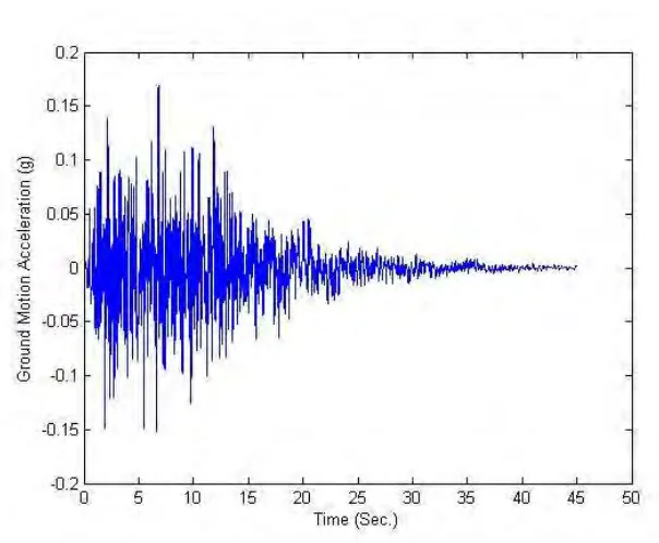
Figure 2.Horizontal (X Direction) Ground Motion Acceleration

To get the frequency content of the ground acceleration, FFT is applied and the Real and Imaginary parts of the results are shown in Figures 3 and 4.

Figure 3.Real part of the Horizontal Ground Motion Acceleration

Figure 4.Imaginary Part of the Horizontal Ground Acceleration

Figure 5.Real Part of the Absolute Acceleration Transfer Function at the ISRS Point Due to Horizontal Ground Motion Acceleration in the X Direction

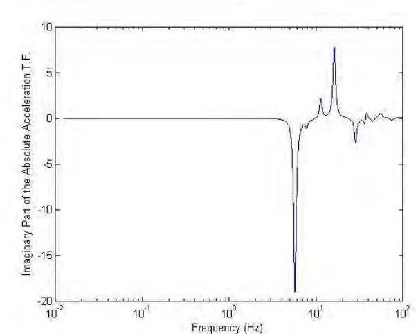
Figure 6.Imaginary Part of the Absolute Acceleration Transfer Function at the ISRS Point Due to Horizontal Ground Motion Acceleration in the X Direction

Figure 7.Real Part of the Absolute Acceleration at the ISRS Location

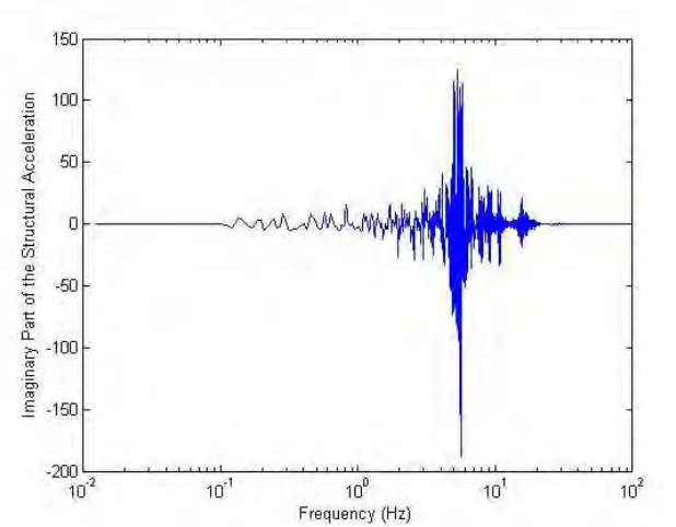
Figure 8.Imaginary Part of the Absolute Acceleration at the ISRS Location

.

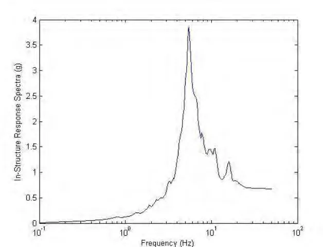
Figure 9.In-Structure Response Spectra for 5% Damping

CONCLUSION

In this paper the application of the frequency domain analysis of structural dynamic problems in the development of In-Structure Response Spectra (ISRS) is presented. This method converts the very tedious time history dynamic analysis to developing the required transfer functions, which is almost like static analysis in the frequency domain, and very fast algorithms of FFT and IFFT. The step by step formulation along with a numerical example of a multistory building in a nuclear facility is illustrated.

NOMENCLATURE

[ ] [ ] [ ]

M

,

C

,

K

Are the mass, damping, and stiffness matrices

[

K

(

i

ω

)

]

Is the dynamic stiffness in the frequency domain

                  • •• U U

U , , Are the relative displacement, velocity, and acceleration vectors in time domain

{ } {

P

(

t

)

,

P

(

i

ω

)

}

Are the load vectors in time domain and frequency domain

ω

Is circular frequency of the load (rad/sec)

      ) (i

ω

U Is displacement vector in the frequency domain

) ( ), (i x t

X

ω

Are input in frequency domain and time domain

) ( ), (i y t

Y

ω

Are output in frequency domain and time domain

) .( .F i

ω

T Is transfer function in the frequency domain

β

Is the ratio of the input frequency to the SDOF natural frequency

[ ]

Γ

Is the influence vector due to specific component of ground motion IFFT

FFT , Are the Fast Fourier Transform and Inverse Fast Fourier Transform IDFT

REFERENCES

ASCE 4-98 (1998), “Seismic Analysis of Safety Related Nuclear Structures and Comments”

Gholampour, A., Ghassemieh, M., Razavi, H., (2011).“A Time Stepping Method in Analysis of Nonlinear Structural Dynamics”, Journal of Applied and Computational Mechanics, Vol. 5, No.2,

Kausel, E., Roesset. J., (1992), “Frequency Domain Analysis of Undamped Systems”, Journal of

Engineering Mechanics, Vol. 118, issue 4, PP 721-734.

MATLAB, (2011), The language of Technical Computing.

Piersol A., Paez, T., (2009), “Harris’ Shock and Vibration Handbook”, Sixth Edition

Razavi, H, Abolmaali, Ali, Ghassemieh, M.,(2007).“A Weighted Average Parabolic Acceleration Time Integration Method for Problems in Structural Dynamics”, Journal of Computational Methods in Applied

Mathematics, Vo. 7, Issue 3, PP 227-238.

Razavi, H., (2002), “A Fast Formulation of Duhamel’s Integral for Problems in Structural Dynamics”,