A new approach to face recognition using Curvelet Transform

University of Windsor University of Windsor

Scholarship at UWindsor

Scholarship at UWindsor

Electronic Theses and Dissertations Theses, Dissertations, and Major Papers

2008

A new approach to face recognition using Curvelet Transform

A new approach to face recognition using Curvelet Transform

University of Windsor

Follow this and additional works at: https://scholar.uwindsor.ca/etd

Recommended Citation Recommended Citation

Mandal, Tanaya, "A new approach to face recognition using Curvelet Transform" (2008). Electronic Theses and Dissertations. 680.

https://scholar.uwindsor.ca/etd/680

A NEW APPROACH TO FACE RECOGNITION USING CURVELET

TRANSFORM

by

Tanaya Mandal

A Thesis

Submitted to the Faculty of Graduate Studies

through Electrical and Computer Engineering

in Partial Fulfillment of the Requirements for

the Degree of Master of Applied Science at the

University of Windsor

Windsor, Ontario, Canada 2008

1*1

395 Wellington Street Ottawa ON K1A0N4 Canada

Bibliotheque et Archives Canada Direction du

Patrimoine de I'edition

395, rue Wellington Ottawa ON K1A0N4 Canada

Your file Votre reference ISBN: 978-0-494-42267-0 Our file Notre reference ISBN: 978-0-494-42267-0

NOTICE:

The author has granted a non-exclusive license allowing Library and Archives Canada to reproduce, publish, archive, preserve, conserve, communicate to the public by

telecommunication or on the Internet, loan, distribute and sell theses

worldwide, for commercial or non-commercial purposes, in microform, paper, electronic and/or any other formats.

AVIS:

L'auteur a accorde une licence non exclusive permettant a la Bibliotheque et Archives Canada de reproduire, publier, archiver,

sauvegarder, conserver, transmettre au public par telecommunication ou par Plntemet, prefer, distribuer et vendre des theses partout dans le monde, a des fins commerciales ou autres, sur support microforme, papier, electronique et/ou autres formats.

The author retains copyright ownership and moral rights in this thesis. Neither the thesis nor substantial extracts from it may be printed or otherwise reproduced without the author's permission.

L'auteur conserve la propriete du droit d'auteur et des droits moraux qui protege cette these. Ni la these ni des extraits substantiels de celle-ci ne doivent etre imprimes ou autrement reproduits sans son autorisation.

In compliance with the Canadian Privacy Act some supporting forms may have been removed from this thesis.

Conformement a la loi canadienne sur la protection de la vie privee, quelques formulaires secondaires ont ete enleves de cette these.

While these forms may be included in the document page count,

their removal does not represent any loss of content from the thesis.

Bien que ces formulaires

Author's Declaration of Originality

I hereby certify that I am the sole author of this thesis and that no part of this

thesis has been published or submitted for publication.

I certify that, to the best of my knowledge, my thesis does not infringe upon

anyone's copyright nor violate any proprietary rights and that any ideas, techniques,

quotations, or any other material from the work of other people included in my thesis,

published or otherwise, are fully acknowledged in accordance with the standard

referencing practices. Furthermore, to the extent that I have included copyrighted

material that surpasses the bounds of fair dealing within the meaning of the Canada

Copyright Act, I certify that I have obtained a written permission from the copyright

owner(s) to include such material(s) in my thesis and have included copies of such

copyright clearances to my appendix.

I declare that this is a true copy of my thesis, including any final revisions, as

approved by my thesis committee and the Graduate Studies office, and that this thesis has

ABSTRACT

Multiresolution tools have been profusely employed in face recognition. Wavelet

Transform is the best known among these multiresolution tools and is widely used for

identification of human faces. Of late, following the success of wavelets a number of new

multiresolution tools have been developed. Curvelet Transform is a recent addition to that

list. It has better directional ability and effective curved edge representation capability.

These two properties make curvelet transform a powerful weapon for extracting edge

information from facial images. Our work aims at exploring the possibilities of curvelet

transform for feature extraction from human faces in order to introduce a new alternative

To

My motherland, India

My parents

&

ACKNOWLEDGEMENTS

I express my deep and sincere gratitude to my advisor, Dr. Jonathan Wu for

giving me this opportunity to work under his supervision; for his guidance, suggestion

and support. I would like to thank my external reader Dr. Nihar Biswas for his priceless

advices. I convey my sincere thanks to my program reader Dr. Huapeng Wu for his

valuable comments. Also I would like to thank my friend Angshul for a conference

publication and for all the technical discussions we had. Special thanks to my mother

Dali Mandal, my father Sankar Mandal, my brother Jeet, my fiance Anirban, my friends

Payel, Shilpi and Sudeepta for their constant support and love. Finally, I take this

opportunity to thank my group members, especially Rashid and Adeel, for their kind

TABLE OF CONTENTS

AUTHOR'S DECLARATION OF ORIGINALITY iii

ABSTRACT iv

DEDICATION v

ACKNOWLEDGEMENTS vi

LIST OF TABLES xii

LIST OF FIGURES xiv

LIST OF ABBREVIATIONS xvi

CHAPTER

1. INTRODUCTION 1

1.1 Introduction to Face Recognition 1

1.2 Challenges in Face Recognition 3

1.3 Objective 4

1.4 Scope of this Work 4

1.5 Thesis Outline 5

2. LITERATURE REVIEW 6

2.1 Introduction 6

2.2 Feature Extraction Approaches 6

2.2.1 Active Appearance Model 7

2.3.1 Holistic Approaches 10

2.3.1.1 Face Recognition by PCA 10

2.3.1.2 Face Recognition by ICA 12

2.3.1.3 Face Recognition by LDA 13

2.3.1.4 Face Recognition by SVM 14

2.3.1.5 Neural Network Approaches 14

2.3.2 Feature Based Methods 15

2.3.2.1 Elastic Bunch Graph Matching 15

2.3.2.2 Hidden Markov Models 15

2.3.3 Hybrid Methods 16

2.3.3.1 Modular Eigenface 16

2.3.3.2 Flexible Appearance Model 16

2.3.3.3 3D Morphable Models 17

2.3.4 Other Approaches 18

3. WAVELET AND CURVELET TRANSFORM 19

3.1 Introduction 19

3.2 Wavelet Transform 19

3.2.1 Continuous Wavelet Transform 21

3.2.2 Discrete Wavelet Transform 22

3.2.3 2D Wavelet Decomposition 22

3.3 Curvelet Transform 24

3.3.2 Fast Discrete Curvelet Transform 25

3.3.3 Application of Curvelets 28

3.4 Wavelet vs. Curvelet 29

4. THE CLASSIFIERS 32

4.1 Introduction 32

4.2 Support Vector Machine 32

4.2.1 Majority Voting with SVM 34

4.2.2 One-Against-All and One-Against-One 34

4.3 ^-Nearest Neighbour Classifier 35

4.3.1 Properties of Jt-NN 35

4.3.2 Distance Measures 36

4.3.3 How to Choose k 37

5. FACE RECOGNITION USING CURVELET FEATURES 38

5.1 Introduction 38

5.2 Datasets 38

5.2.1 AT&T "The Database of Faces" 38

5.2.2 Georgia Tech Database of Faces 39

5.2.3 Essex Grimace Database 40

5.3 Curvelet Based Feature Extraction 40

5.3.1 Recognition using Simple Curvelet Features and ANN 43

5.3.1.2 Experiments on AT&T Database 46

5.3.1.3 Experiments on Georgia Tech Database 47

5.3.1.4 Comparison with Wavelets 47

5.3.1.5 Discussion 50

5.3.2 Recognition using Bit Quantization, Curvelet Features and SVM... 51

5.3.2.1 Experiments on Essex Grimace Database 53

5.3.2.2 Experiments on AT&T Database 54

5.3.2.3 Experiments on Georgia Tech Database 55

5.3.2.4 Comparison with Wavelets 55

5.3.2.5 Discussion 57

6. FACE RECOGNITION USING CURVELET SUBSPACES 58

6.1 Introduction 58

6.2 Datasets 58

6.2.1 JAFFE Database 58

6.2.2 Faces94 Database 59

6.3 Recognition using Curvelet Subbands 60

6.3.1 Recognition using Curvelet Subbands and PCA 60

6.3.1.1 Results for Essex Grimace Database 64

6.3.1.2 Results for JAFFE Database 65

6.3.1.3 Results forFaces94 Database 66

6.3.1.4 Comparison Wavelet-based PCA and Traditional

6.3.1.5 Discussion 68

6.3.2 Recognition using Discriminant Curvelet Features 69

6.3.2.1 Results for Essex Grimace Database 71

6.3.2.2 Results for JAFFE Database 72

6.3.2.3 Results for Faces94 Database 73

6.3.2.4 Comparison with Discriminant Wavelet Method 73

6.3.2.5 Discussion 75

7. CURVELETS AND WAVELETS: A COMBINED APPROACH 76

7.1 Introduction 76

7.2 Recognition using Curvelets and Wavelets 76

7.2.1 Experimental Results 78

7.2.2 Discussion 80

7.3 Comparative Study 81

8. CONCLUSION 84

8.1 Contribution 84

8.2 Future Work 85

REFERENCES 86

APPENDIX A 91

APPENDIX C 96

LIST OF TABLES

Table 2.1: Classification of Face Recognition Techniques 9

Table 5.1: Curvelet based results for Essex Grimace 45

Table 5.2: Curvelet based results for AT&T 46

Table 5.3: Curvelet based results for Georgia Tech 47

Table 5.4: Comparison with wavelet based results on Essex Grimace 48

Table 5.5: Comparison with wavelet based results on AT&T 49

Table 5.6: Comparison with wavelet based results on Georgia Tech 50

Table 5.7: Curvelet based results for Essex Grimace 53

Table 5.8: Curvelet based results for AT&T 54

Table 5.9: Curvelet based results for Georgia Tech 55

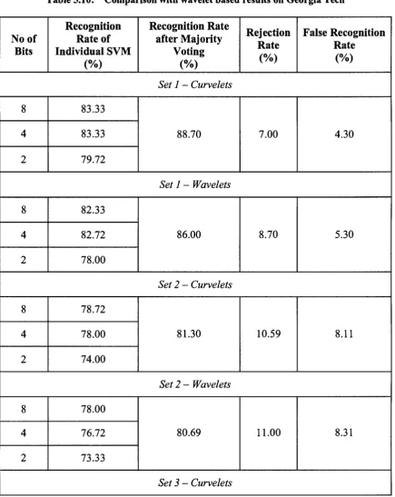
Table 5.10: Comparison with wavelet based results on Georgia Tech 56

Table 6.1: Curvelets & PCA based results for Essex Grimace 64

Table 6.2: Curvelets & PCA based results for JAFFE 65

Table 6.3: Curvelets & PCA based results for Faces94 67

Table 6.4: Discriminant curvelet based results for Essex Grimace 71

Table 6.5: Discriminant curvelet based results for JAFFE 73

Table 7.1: Results for Combined Approach on AT&T 80

Table 7.2: Comparative Study 82

Table I: Curvelet Based Results for JAFFE 91

Table II: Comparison with Wavelets on JAFFE 92

Table III: Curvelet Based Results for Faces94 93

Table IV: Comparison with Wavelets on Faces94 94

Table V: Results for AT&T 95

LIST OF FIGURES

Figure 1.1: A Generic Face Recognition System 2

Figure 2.1: Active Appearance Model 8

Figure 2.2: Eigenfaces 12

Figure 2.3: Flexible Appearance Model 17

Figure 3.1: Shifting of Wavelet 20

Figure 3.2: Scaling of Wavelet 21

Figure 3.3: 2D 1-level Wavelet Decomposition 23

Figure 3.4: Left - Original Lena Image; Right - 3-level Wavelet Decomposition 23

Figure 3.5: A Few Curvelets 25

Figure 3.6: Curvelets in Fourier Frequency (left) and Spatial domain (right) 26

Figure 3.7: Contrast Enhancement by Curvelets 28

Figure 3.8: Image Denoising by Curvelet Transform 28

Figure 3.9: Edge Representation by Wavelet and Curvelet Transform 30

Figure 4.1: Support Vector Classification 33

Figure 4.2: Effect of A:-value 37

Figure 5.1: Sample Images from AT&T Database 39

Figure 5.2: Sample Images from Georgia Tech Database 40

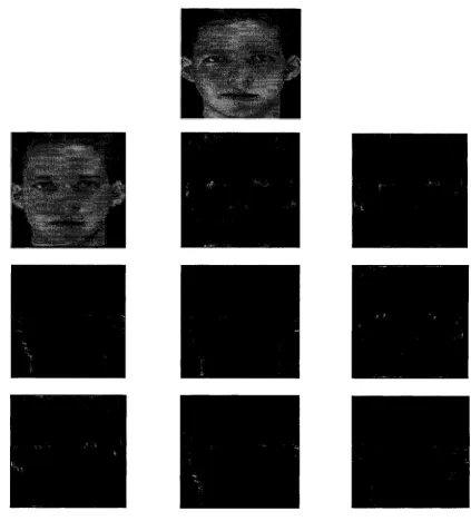
Figure 5.4: Curvelet Transform of Faces: 1st image is the original image, 1st image in

the 2nd row is the approximate coefficients and others are detailed

coefficients at eight angles 42

Figure 5.5: The images in the first column are the original 8-bit representations; the

images in the second column are the 4 bit images while the last ones are 2

bit representations 52

Figure 6.1: Sample Images fron JAFFE Database 59

Figure 6.2: Sample Images from Faces94 Database 59

Figure 6.3: Curveletfaces: 1st image in the 1st row is the original image; 2nd image in

the 1st row is the approximate coefficients and others are detailed

coefficients at eight angles 61

Figure 6.4: Curvelet Based PCA face Recognition Scheme 62

Figure 6.5: Comparison with wavelet based PCA and traditional PCA on JAFFE....67

Figure 6.6: Comparison with wavelet based PCA and traditional PCA on Faces94..68

Figure 6.7: Recognition Scheme for Discriminant Curvelet Features 69

Figure 6.8: Comparison with discriminant wavelet based results on JAFFE 74

Figure 6.9: Comparison with discriminant wavelet based results on Faces94 75

LIST OF ABBREVIATIONS

Active Appearance Model

Active Shape Model

Convolution Neural Network

Continuous Wavelet Transform

Discrete Cosine Transform

Dynamic Link Architecture

Elastic Bunch Graph Matching

Evolution Pursuit

Fast Discrete Curvelet Transform

Fast Fourier Transform

Fisher Linear Analysis

Fisher Linear Discriminant

Hidden Markov Model

Independent Component Analysis

Japanese Female Facial Expression

Kernel Principal Component Analysis

Kerhunen-Loeve

k Nearest Neighbour

Linear Discriminant Analysis

Linear Fisher Analysis

NFL:

NFP:

NFS:

OAA:

OAO:

ORL:

PCA:

PDBNN:

NN:

SOM:

STFT:

SVM:

USFFT:

Nearest Feature Line

Nearest Feature Plane

Nearest Feature Space

One Against All

One Against One

Olivetti Research Labrotary

Principal Component Analysis

Probability Decision Based Neural Network

Neural Network

Self Organizing Map

Short Time Fourier Transform

Support Vector Machine

CHAPTER 1

INTRODUCTION

1.1 Introduction to Face Recognition

Face Recognition can be defined as a problem of identifying or verifying a

person from still images or video sequences using a stored database of facial images.

Usually, the input to a face recognition system is an unknown face; in identification

problems, the system retrieves the identity of the input face from the database of known

individuals; whereas in verification problems the system either accepts or rejects the

claimed identity of the query face. Face recognition has been studied for more than 30

years now and it has emerged as one of the most successful applications of image

analysis. Due to the growing interest in biometrics authentication, it has become a

popular research area not only in the field of computer vision, but in neuroscience and

psychophysics as well. Unlike other biometrics (fingerprints, iris etc.) face recognition is

non-intrusive i.e. images can be taken, identified or verified even without the knowledge

of the subject. Moreover, the data required for the system is human readable and can be

collected easily with simple devices like camera. Face recognition has become a major

issue especially in the past decade, due to its important real-world applications in areas

like video surveillance, smart cards, database security, telecommunication, digital

Broadly, face recognition techniques can be divided into two categories,

depending upon the type of images (still or video) being used in the recognition system.

Our work is confined to recognition of faces from still images only. Usually, the available

images are 2D intensity images of human faces, which are 3D objects. So this problem

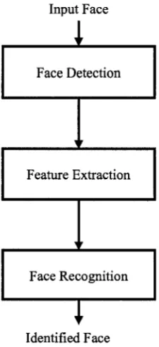
can be seen as a problem of recognising 3D objects from 2D images. A fully automatic

face recognition system must perform the following three subtasks: face detection,

feature extraction and recognition/identification. However, each of these subtasks itself is

a separate area of research and concentrating on all of them simultaneously is difficult.

Isolating the subtasks not only simplify our job but also enhance the assessment and

advancement of the component techniques. So, instead of detecting faces from images,

standard databases of faces have been used for the experiments; and our prime focus has

been developing a new efficient feature extraction technique.

Input Face

1

i '

Feature Extraction

i '

Face Recognition

1.2 Challenges in Face Recognition

Faces are specific objects, that look similar from its most common appearance

(frontal faces), but subtle features make them different. We, human beings, recognize

faces with natural ease; but machine recognition of faces is a challenging job. The

advantage of computer face recognition system is its capacity to handle large number of

faces where human brain has limited memory i.e. capacity to remember faces. However,

there are various problems associated with automatic face recognition; they are listed

below:

• Head pose: Rotation or tilt of the head; even if the appearance is frontal, it affects

the performance of the recognition system significantly.

• Illumination change: The direction of light illuminating the faces greatly affects

the recognition accuracy. It has been noticed that illuminating a face image

bottom up reduces the accuracy of the system.

• Facial expression change: From minor expression changes like smiling to

extreme expression variations like shouting or crying or making grimaces, tend to

affect the recognition rate of a system largely.

• Aging: Images taken at long interval or even at different days may seriously affect

the correct recognition rate of a system.

• Frontal vs. Profile: Profile images can be difficult to recognize, when mostly

frontal faces are available for matching.

• Occlusion: Even partial occlusion of faces due to objects or accessories like

sunglass or scarf, makes identification a difficult task.

Other issues with face recognition are: (i) it is not as accurate as other biometrics

like fingerprints or iris recognition, (ii) optimum size of the facial images to be used is

still an open issue to researchers, (iii) the problem with accurate feature localization.

Though, static image based face recognition has attained a certain level, but still far away

from the capability of human perception.

1.3 Objective

Feature extraction is a key step prior to recognition and an effective feature

extraction method can greatly enhance the performance of any face recognition system

both in terms of accuracy and speed. The features extracted from facial images can be

local (lines, curves, edges etc.) or facial features (eyes, nose mouth etc.). This study aims

at developing a novel face recognition technique from static images, employing a new

multiresolution analysis tool called digital curvelet transform for feature extraction. The

feature extraction method proposed in this thesis is a generic method which is based on

capturing information about the local features like edges, curves etc.

1.4 Scope of this Work

A novel approach towards human face recognition based on a multiresolution

analysis tool named digital curvelet transform is discussed in this thesis. This work

includes the following studies:

• Face recognition using curvelet transform and k-NN classifier; comparison with

• Application of curvelet transform on bit quantized images and recognition using

SVM classifier; comparison with results achieved using wavelet transform.

• Combination of curvelet features and PCA; comparison with existing techniques

like traditional PCA and wavelet-based PCA.

• Combination of curvelet features with LDA; a comparative study with

wavelet-based LDA method.

• A combined approach using both curvelet and wavelet transform, incorporating a

PCA+LDA framework.

• Comparative study of proposed curvelet based methods with published work.

1.5 Thesis Outline

This thesis is organized into eight chapters. Chapter 1 provides a general

introduction to face recognition, the challenges associated with this problem, the

objectives and scope of the thesis. In Chapter 2 a detail review of previous work on face

recognition can be found. Chapter 3 presents a theoretical description of wavelet

transform and curvelet transform; as well as discusses why curvelet transform should be

able to provide an effective means for feature extraction from face images. Chapter 4

aims at giving an overview of the classifiers that have been used for the identification

task. Chapters 5, 6 and 7 explain the proposed methods and list the experimental results

along with the comparative studies. Chapter 8 summarizes the contributions and indicates

the scope of future work. Some additional information has been provided in the

CHAPTER 2

LITERATURE REVIEW

2.1 Introduction

The earliest work on face recognition has been found to take place in 1950s in

the field of psychology by Bruner and Tagiuri and in engineering by Bledsoe in 1960s. In

1970s, Kelly and Kanade started the research on automatic machine recognition of faces

[1]. Since 1990s face recognition has become popular in different fields like computer

vision, neuroscience, psychophysics etc. This field has grown fast and significantly in the

past decade due to increased interest in commercial opportunities, availability of

real-time hardware and importance in surveillance related applications.

Various techniques and algorithms have been developed by researchers. A

comprehensive survey of all those techniques is out of the scope of this thesis. Interested

reader can refer to the works of Zhao et al. [1] and Gross et al [2]. Since this work is

restricted to the use of static images, the current chapter provides a detailed review on the

still-image based face recognition research.

2.2 Feature Extraction Approaches

face recognition system. The features extracted from facial images are either local (lines,

curves, edges etc.) or facial features (eyes, nose mouth etc.). Grossly, feature extraction

techniques can be divided into three categories [1]:

• Generic Methods - based on edges, lines and curves.

• Feature-Template Based Methods - deals with detection of facial features like

eyes, nose, mouth etc.

• Structural Matching Methods - a statistical method which takes geometrical

constraints into consideration.

Early face recognition researchers focused on individual features, such as locating

the position of eyes; later, structural matching methods were found to be more reliable. A

successful example of such a statistical method is Active Appearance Model introduced

by Cootes et al. [3] in 2001; this method is briefly discussed below.

2.2.1 Active Appearance Model [3]

A statistical model called 'Active Appearance Model' (AAM) [3] was

suggested by Cootes et al. in 2001. This model is basically a combination of a shape

model called Active Shape Model or ASM [4] and a model of appearance variation of

shape free textures. A training set of 400 facial images, each manually labelled with 68

landmark points and 10,000 intensity values sampled from different facial images have

been used for this work. Then, a shape model is constructed using each set of landmark

points as a vector and applying PCA; a shape model consists of mean shape, orthogonal

mapping matrix Ps and projection vector bs. Each sample image is warped to match its

information. A texture model, consisting of mean texture, orthogonal mapping matrix Pg

and projection vector bg, was constructed using PC A. To correlate between shape and

texture variation, PCA is applied for the third time on the concatenated vectors bs and bg.

In this combined model, a vector c controls shape and texture of the model. While

matching an image with the model, an optimal vector of parameters is searched by

minimizing the difference between the synthetic images and the given one. After

matching, a best fitting model is generated, which actually gives the exact locations of all

the facial features.

Set of landmark points

s = s + Psb-K

g — I + Pgbg

b

P C ^

Shape Free Patch

Figure 2.1: Active Appearance Model [3]

2.3 Face Recognition Approaches

Various face recognition techniques have been discussed in [1] and [2]. In the

work of Zhao et al. face recognition methods are divided primarily into following three

categories; table 2.1 shows the detail classification:

• Feature Based or Structural Methods - for these approaches, the local features

such as eyes, nose, mouth etc are extracted and their location and statistical

information are fed to a structural classifier.

• Hybrid Methods - these methods use both the local features and the whole face

region for recognition.

Table 2.1: Classification of Face Recognition Techniques [1]

Approach

Holistic Approaches

Principal Component Analysis (PCA)

Eigenface

Fisherface

SVM

ICA

Other Representations

LDA/FLA

PDBNN

Feature based methods

Pure geometry methods

Dynamic Link Architecture

Convolution Neural Network

Hybrid Methods

Modular Eigenface

Hybrid LFA

Component based

Representative Works

Direct application of PCA

FLD on eigenspace

Two-class problem based on SVM

ICA based feature analysis

FLD/LDA on raw images

Probabilistic decision based NN

Earlier methods, recent methods

Graph Matching methods

SOM learning based CNN methods

Eigenface & eigenmodules

Local & global feature methods

2.3.1 Holistic Approaches

2.3.1.1 Face Recognition by PCA

PCA is a useful tool to obtain a lower dimensional representation of data. It is

used not only to reduce statistical redundancy; but to reduce the system's sensitivity to

noise (for example blurring, partial occlusion, change of background etc.) as well.

Various face recognition algorithms have been proposed based on PCA. A brief overview

of PCA is given here for ready reference [5, 6].

Let X = {Xn eRd \n = 1,2 N) be an ensemble of vectors, which is formed

by converting each of the images to a vector by row concatenation, with d being the

N

product of the width and height of an image. Let E(x) = 1/N ^ X n be the average

n = l

vector in the ensemble. After subtracting the average from each element of X, we get a

modified ensemble of vectors.

X = {X„,n = L2...JV} with X„ = X-E(x) (2.1)

The covariance matrix M for the ensemble X is defined by

M = cov( X) = E(X ® X) (2.2)

where, M is a d x d matrix, with elements

M{i,j) = \INfd[Xn{i)Xn{j)-\,\<i,j<d (2.3)

It is well known from matrix theory that the matrix M i s positively definite (or

semidefinite) and has only real non-negative eigenvalues [5]. The eigenvectors of matrix

Sirovich and Kirby first used K-L transform to present human faces. Afterwards Turk and

Pentland developed a PC A based face recognition system in 1991.

The work of Turk and Pentland [8] was motivated by that of Sirovich and

Kirby. In their work, each of the training images was converted to a vector by row

concatenation. The entire set of training images thus constructed the covariance matrix.

This covariance matrix was solved for eigenvectors and eigenvalues. Then n best

eigenvectors associated with n largest eigenvalues were selected; these eigenvectors were

named 'eigenfaces'. This method claimed that each face can be represented as a weighted

combination of selected eigenvectors or eigenfaces. The classification task was

performed using nearest neighbour classifier. This method was found to be robust to

illumination changes but performed weakly with scale variation.

Later, the work of Turk and Pentland was extended to a Bayesian approach by

Moghaddam and Pentland in 1997 [9]; in their system the simple eigenspace based

method was extended to use probabilistic measure of similarity. However, this scheme

suffers from the problem of estimating probabilistic distributions in a high dimensional

space from limited number of training examples per class [1]. In [10] Moghaddam argued

Bayesian approach to be superior in terms of simplicity, computational efficiency and

performance over PCA, ICA and nonlinear Kernel PCA (KPCA), where he examined

Figure 2.2: Eigenfaces [8]

PCA has now become one of the most popular tools for dimensionality

reduction. Though this is widely used, it has two major drawbacks: high computational

complexity and low discriminatory power. However, Chung et al. [11] suggested the use

of Gabor Filter in combination with PCA in order to overcome the shortcomings of PCA.

The authors of [11] argued that when raw images are subjected to PCA, the correlation of

facial features is not well-reflected in eigenspace. So, they suggested using Gabor filter to

extract facial features and then use PCA to classify the features optimally. It has been

claimed that several problems like, deformation of face images due to in-plane in-depth

rotation, illumination and contrast variation can be solved by extracting facial features

using Gabor Filters.

2.3.1.2 Face Recognition by ICA

Independent Component Analysis is a generalization of Principal Component

Analysis. ICA is argued to have the following advantages over PCA:

• ICA finds a not-necessarily orthogonal basis which can reconstruct the data better

than PCA, even in the presence of noise.

• ICA is sensitive to higher order statistics of the data, not only covariance matrix.

Based on the above arguments, ICA has been used to extract features for face recognition

by Bartlett et al. [12] in 1998 and performance improvement over PCA based method

was reported.

2.3.1.3 Face Recognition by LDA

Linear Discriminant Analysis or Fisher Discriminant Analysis has also been

successfully applied in face recognition by researchers [13]. LDA has been found to

improve the classification accuracy of a system, when more than one image is available

per class. LDA based recognition method aims at maximizing between-class scatter

simultaneously minimizing within-class scatter. LDA training is performed via scatter

matrix analysis [14]. For an N-class problem, the between and within class scatter matrix,

Sb and Sw respectively, are calculated as follows:

^ = E ^ K X «(- » o ) ( »;- » o )r (2-4)

^ w = ZPr ( w , ) C , (2-5)

i = l

where Pr (w,) is prior class probability, ni is conditional mean vector, n0 is overall mean

vector and Ci is average scatter of the sample vectors. Methods of combining PCA and

LDA have been studied in [15, 16]. For this purpose first the face images are projected

into eigenspace and then eigenspace projected vectors are again projected to LDA

2.3.1.4 Face Recognition by SVM

Support Vector Machine or SVM was employed as a classifier to recognize

human faces by Phillips in 1998 [17]. Given a set of points, SVM finds the optimal

'hyperplane'. A hyperplane separates the data points into two classes and at the same

time maximizes the distance from either class. This also indicates that SVM is a binary

classifier whereas face recognition is a multi-class problem. The faces were projected in

difference space where it can be considered as a two-class problem.

2.3.1.5 Neural Network Approaches

Neural Network based approaches have also been very popular in addressing

the problem of face recognition. Neural networks have found their application in both

holistic and feature-based approaches. Probability Decision Based Neural Network

(PDBNN) method by Lin et al. [18] and Evolution Pursuit (EP) by Liu and Wechsler [19]

are two successful examples of neural network approaches applied holistically. The

PDBNN method is described here briefly.

PDBNN is an extension of DBNN proposed by Kung and Taur in 1995 [20];

PDBNN has three modules: face detector, eye localizer and face recognizer. Unlike other

methods, this technique only considers the upper part of faces (eyebrows, eyes and nose,

not mouth) in order to make the system robust to facial expression. The speciality of this

method is its modularity i.e. for each class or person PDBNN dedicates one of its subnets

for the representation of that particular person. Two sets of features are constructed from

the segmented facial regions at reduced resolution and these two features are fed to two

2.3.2 Feature Based Methods

Many feature based methods have been proposed till date. Some methods made

use of geometry of local features, some used Hidden Markov Models (HMM) or

Bayesian classifiers. Elastic Bunch Graph Matching (Okada et al. 1990 [21], Wiskott et

al. 1997 [22]) is one of the most widely known algorithms of this kind.

2.3.2.1 Elastic Bunch Graph Matching

This technique is based on Dynamic Link Architecture or DLA (Buhmann et al.

1990 [23], Lades et al. 1993 [24]). DLA differs from traditional artificial neural network

by the fact that syntactical relationships in neural network can be represented by DLA.

Both Buhmann et al. and Lades et al. used Gabor wavelets to extract features (called

'jets'), which were locally estimated and were found robust to illumination changes,

translation, distortion, scaling and rotation. 'Jets' [21] are small patches of grey values in

an image around a pixel, which are based on wavelet transform and can be defined as a

convolution of the image with a family of Gabor kernels [22]

- k 2 ( k2x2^

2(T 2

a2

exp(ikjX) - exp( ) (2.6)

A set of such jets (called 'bunch graph representation') was constructed from different

facial images. EBGM based methods have been successfully applied in the areas of face

detection, gender classification, pose estimation and object recognition.

2.3.2.2 Hidden Markov Models

HMM was applied for feature extraction and face identification by Samaria et

intuitively divided into components such as forehead, eyes, nose, mouth and chin. These

were considered as strips of pixels. Nefian et al. in 1998 reported better performance

using KL projection instead of using raw pixel values. The recognition accuracy of HMM

using ORL database [59] was found to be 87%. Later using 2D HMM [27] recognition

performance was improved to 95%.

2.3.3 Hybrid Methods

2.3.3.1 Modular Eigenface

These methods use local features along with the entire face region. Modular

Eigenface [28] by Pentland et al. 1994 is an example of hybrid methods where the global

eigenfaces as well as the local eigenfeatures were used for identification. The concept of

eigenfaces was extended to eigenfeatures, namely eigeneyes, eigenmouth etc.

Recognition performance was computed as a function of eigenvectors, both for

eigenfeatures alone and for combined representation. For lower-order spaces,

eigenfeatures were found to be more effective compared to eigenfaces and the

combination showed a marginal improvement only.

2.3.3.2 Flexible Appearance Model

Flexible appearance model [29] was used for automatic face recognition by

Lanities et al. in 1995. Both shape and grey-level information had been used for

recognition. The shape information was captured using Active Shape Model. To increase

image, three types of information, including shape parameters, shape-free image

parameters and local profiles have been used for classification.

*Hstiraep S i p w&M fluted : o * r a § i m mma shape

• , , . . , j .

f f T

jciasteitjoa

Figure 2.3: Flexible Appearance Model [1]

2.3.3.3 3D Morphable Models

Recently 3D Morphable models [30] by Blanz et al. 1999 and component-based

recognition methods [31] by Heisele et al. 2001 have become quite popular. The key idea

of component-based methods is to decompose the face into a number of facial

components that are interconnected by a flexible geometric model. The system believes

that by using components the pose change due to head movement can be accounted for.

However, the method requires a large number of samples to work successfully.

3D Morphable Models have better ability to deal with the head pose and

face images (frontal, semiprofile and profile) per person to compute the 3D face model.

From this 3D face model synthetic images are generated. For face recognition nine facial

components were used along with the entire face image, where as for face detection

fourteen facial components were used. SVM was used as a classifier and recognition

accuracy reported is quite high.

2.3.4 Other Approaches

Discrete Cosine Transform (DCT) and Fourier Transform have been applied to

face recognition problem in [32] and [33] respectively. In [32] the authors tried to detect

some critical areas of the facial images. The method was based on matching the image to

a map of facial attributes associated with specific areas of face. DCT has also been used

in combination with HMM in [34]. Spies and Ricketts in [33] used Fourier spectra for

face analysis.

Most of the methods discussed above use frontal images. Liposcak et al. [35]

have worked on profile images based on the original and morphological representation of

derived profile shapes. They converted the grey-scale images to binary images. After

normalization, they simulated the hair growth and haircut to derive two more profile

silhouettes. Feature vectors extracted from these three profile images were used for

recognition. 3D range images (obtained using laser scanner) have also been used as an

input to face recognition system [2]. Infrared scanning of face images has been utilized in

[36]. Some significant recent developments in face recognition field include 2D PC A

CHAPTER 3

WAVELET AND CURVELET TRANSFORM

3.1 Introduction

Multiresolution analysis tools such as Wavelet Transform have already been

proved quite useful for analyzing the information content of images; and hence they have

found their application in areas like image processing, pattern recognition and computer

vision. This chapter discusses Wavelet Transform, the best known multiresolution tool

and Curvelet Transform, a new multiresolution analysis tool used in this work. The

underlying theory of both the transforms have been studied. The description of Wavelet

Transform has been kept short as it is quite well-known and discussed in numerous books

and research articles.

3.2 Wavelet Transform

Wavelet is a widely known multiscale transform, which is capable of providing

the time and frequency information of a signal simultaneously. Fourier analysis of a

signal enables us to represent a signal by the sum of a series of sines and cosines. But,

Fourier expansion has only frequency resolution but no time resolution. Wavelet

Transform, developed to overcome the limitations of Short Time Fourier Transform

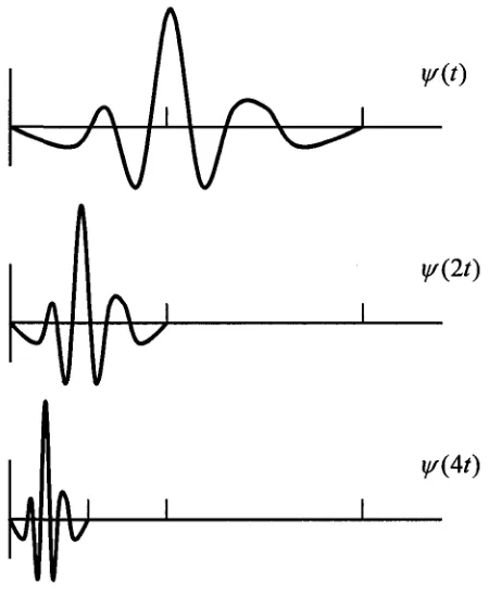
In wavelet analysis a signal is processed at different scales or resolutions. The

signal is cut up into different frequency components by a wavelet prototype function and

each of the components is studied with a resolution matched to its scale. This wavelet

prototype function y/{t) is called 'mother wavelet', as other wavelets are generated from

this single basic wavelet by translation and scaling [40]. A wavelet function can be

defined as a waveform of limited duration which has an average value of zero. As the

original signal can be represented in a linear combination of such wavelet functions,

further operations on the signal can easily be performed using just the corresponding

wavelet coefficients.

It is worth mentioning that higher scale means more 'stretched' wavelets. More

stretched the wavelet, longer the portion of signal it's being compared with, hence

coarser the resolution. On the other hand lower scale corresponds to more 'compressed'

wavelet, which in turn corresponds to rapidly changing details of the signal.

y/(t-k)

j / ( 2 0

W{At)

Figure 3.2: Scaling of Wavelet

3.2.1 Continuous Wavelet Transform

Continuous Wavelet Transform or CWT can be defined as the sum over entire

time of the signal fit) multiplied by scaled, shifted versions of wavelet

function y/(t) [39].

W(s,r)= jfiOvliWt

Equation 3.1 shows how a signal fit) can be decomposed by a set of basis

functions y/ST it), called wavelets. Here, s and r corresponds to scale and translation

respectively. The wavelets y/ST it) are generated from mother wavelet function y/it) by

1 ft-T^

VI

¥„(*) =-TV <3'2)

v s J

3.2.2 Discrete Wavelet Transform

CWT can operate at any possible scale; but computing wavelet coefficients at

every possible scale is tedious and impractical. So some particular values of scale and

position have to be chosen. Generally a didactic scale is chosen and using this, accurate

results can be achieved. This is called Discrete Wavelet Transform. This is obtained by

modifying the wavelet representation in (3.2) [39] as follows

1

J' I t

t IX L rt tJ rt

(3.3)

44 I

i J

Here j and k are integers and s0 > 1 is a fixed dilation step. T0 is the translation factor

and depends upon dilation step.

3.2.3 2D Wavelet Decomposition

As this work deals with images i.e. 2D signals, 2D wavelet decomposition

becomes an important topic of discussion. Wavelet decomposition can be regarded as the

projection of a signal on the set of wavelet basis vectors. Two dimensional wavelet

transform is derived from two ID wavelet transform by taking tensor products [6]. It is

implemented by applying ID wavelet transform to the rows of the original (image data in

this case) data and to the columns of the row transformed data. When wavelet transform

XL

:HL.

LH

HH

Figure 3.3: 2D 1-Ievel Wavelet Decomposition

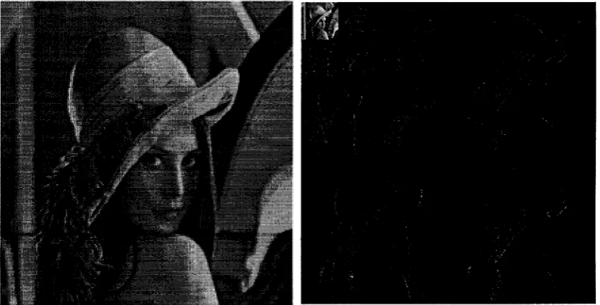
LL is a coarser approximation of the original image data. LH, HL and HH

correspond to horizontal, vertical and high frequency changes of the data. Figure 3.3

shows 1-level decomposition. Further decomposition can be carried out on LL subband.

Figure 3.4 shows a 3-level wavelet decomposition of the original 'lena' image (left). One

of the advantages of wavelet decomposition is that, it provides local information in both

frequency and space domain.

3.3 Curvelet Transform

Over the past two decades, following the success of wavelets, other

multiresolution tools like contourlets, ridgelets etc. were developed. "Curvelet

Transform" is a recent addition to this list of multiscale transforms [41-43]. It was

developed by Candes and Donoho in 1999. The development of curvelet transform was

motivated by the need of image analysis [41]. This transform has improved directional

capability, better ability to represent edges and other singularities along curves as

compared to other traditional multiscale transforms, e.g. wavelet transform.

3.3.1 First Generation Curvelets

Curvelet construction is based on combining several ideas [41]:

• Ridgelets - a method of analysis suitable for objects with discontinuities along

straight lines

• Multiscale Ridgelets - a pyramid of windowed ridgelets, renormalized and

transported to a wide range of scales and locations

• Bandpass Filtering - separates an object out into a series of disjoint scales.

Curvelet Transform is based on above mentioned multiscale ridgelets. In combination

with these, spatial bandpass filtering is used to isolate different scales. Curvelet

coefficients are of two types: at coarse scale they are called 'wavelet scaling function

coefficients' and at fine scale they are called 'multiscale ridgelet coefficients' of

bandpass filtered object. Like ridgelets, curvelets can occur at any scale, location and

the relationship between width and length can be expressed as width «length2 and

anisotropy increases with decreasing scale obeying power law [42]. Figure 3.5 shows

how curvelets look like at different scales, locations and orientations.

Figure 3.5: A Few Curvelets at different scale, position and angle [42]

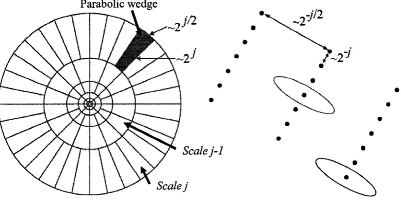
3.3.2 Fast Discrete Curvelet Transform

In past few years curvelet construction has been redesigned in order to make it

simpler to understand and use. This second generation curvelet transform [44] is not only

simpler, but is faster and less redundant compared to its first generation versions

discussed in previous section. In order to implement curvelet transform, first of all a 2D

FFT of the image is taken. Then the 2D Fourier Frequency Plane is divided into

'parabolic' wedges. Finally an inverse FFT of each wedge is taken to find the curvelet

of the Fourier Frequency plane in its left image; the right one represents curvelets in

spatial Cartesian grid associated with a given scale and orientation [44]. From the right

image, it can also be seen that curvelets are thin elliptical in shape; due to the parabolic

relation between their width and length, they take the shape of elongated needles.

Figure 3.6: Curvelets in Fourier Frequency (left) and Spatial domain (right) [44]

There are two different digital implementations:

• Curvelets via USFFT (Unequally Spaced Fast Fourier Transform)

• Curvelets via Wrapping.

Though both the implementations use the same digital coronization but differ in the

choice of spatial grid. Both of the FDCTs run in 0(n2 log«) flops for n by n Cartesian

arrays [44]. Letf[tl,t2],0<tl, t2<n be a Cartesian array and let /[«,,n2]denote its

Pj = {(nx,n2):nX0 <nx <nl0 + LXJ,n20 <n2 <n2fi+L2J) (3.4)

Both the FDCT algorithms are described below.

Algorithm for FDCT via USFFT [44]:

1. Apply 2D FFT and obtain Fourier samples f[nx ,n2], - nl2< nx, n2 < nil.

2. For each scale/angle pair (_/,.£), resample (or interpolate) f[nx,n2]to obtain

sampled values f\nx, n2 -nx tan 9t ] for (nx, n2) e P^.

3. Multiply the interpolated (or sheared) object / w i t h the parabolic windowUJ}

effectively localizing / near the parallelogram with orientation^, and obtain

fj,t[ni,n2] = f[ni,n2-nlianet]Uj[n1,n2]. (3.5)

4. Apply the inverse 2D FFT to each fjt, hence collecting the discrete coefficients.

Algorithm for FDCT via Wrapping [44]:

1. Apply 2D FFT and obtain Fourier samples / [ « , ,n2], -nl2<nx, n2 <nl2 .

2. For each scale j and angled , form the productC/^. ^[wj, n2 ]f[n{, n2] .

3. Wrap this product around the origin and obtain

fjJ[n1,n2] = W(UJJ)[nl,n2], (3.6)

where the range nx and n2 is now 0 < nx < LXj and 0 < n2 < L2j.

3.3.3 Application of Curvelets

Curvelets, being a new concept, has not yet been very popular. So far, it has

been successfully applied mostly in the fields of image processing, like image denoising

[42], image compression [45], image fusion [46], contrast enhancement [47], image

deconvolution [48], high quality image restoration [49], astronomical image

representation [50] etc. Recently curvelets have also been employed to address a few

problems of computer vision and patter recognition, like Optical Character Recognition

[51], finger-vein pattern recognition [52] and palmprint recognition [53].

3.4 Wavelet vs. Curvelet

The sparsity of Fourier series is destroyed due to discontinuities (Gibbs

Phenomenon); it requires a large number of terms to reconstruct a discontinuity in

Fourier series within good accuracy. Later, wavelets are found to have the ability to solve

the problems of Fourier series, as they are localized and multiscale. However, though

wavelets do work efficiently in one-dimension, they fail to represent higher dimensional

singularities effectively due to limited orientation selectivity. Wavelets and related

classical multiresolution ideas exploit a limited dictionary made up of roughly isotropic

elements occurring at all scales and locations [54]. These dictionaries do not exhibit

highly anisotropic elements and there are only a fixed number of directional elements

(The standard orthogonal wavelet transforms have wavelets with primarily vertical,

primarily horizontal and primarily diagonal orientations) independent of scale. Images do

not always exhibit isotropic scaling and thus these limitations of wavelets call for other

kinds of multi-scale representation.

The most interesting fact about curvelets is that it has been developed specially

to represent objects with 'curve-punctuatedsmoothness' [54] i.e. objects which display

smoothness except for discontinuity along a general curve; images with edges would be

good example of this kind of objects. Wavelet transform has been profusely employed to

address different problems of pattern recognition and computer vision because of their

capability of detecting singularities. But, though wavelets are good at representing point

singularities in both ID and 2D signals, they fail to detect curved singularities efficiently.

Figure 3.9 shows the edge representation capability of wavelet (left) and curvelet

required for an edge representation than that compared to the number of required

curvelets, which are of elongated needle shape. Roughly, to represent an edge of squared

error 1/iV, 1/N wavelets but only 1 /-JN curvelets [55] are required. One more novelty

of curvelet transform is that it is based on anisotropic scaling principal, where as wavelets

rely on isotropic scaling.

Figure 3.9: Edge Representation by Wavelet and Curvelet Transform [56]

Let us consider a function/, which has a discontinuity across a curve and is

otherwise smooth; if it is approximated by the best m terms in Fourier expansion, the

squared error is given by [56]

/ - / . ccm 1/2, m -»+oo (3.7)

For wavelets,

J J m ccm , m -> +oo (3.8)

~ 2

/ - /mc oc log(w)3m~2, m ->• +00 (3.9)

To summarize, wavelet transform suffers from the following limitations:

• Edge representation - though wavelets perform better that FFT, it is not optimal.

• Limited number of directional elements independent of scale

• No highly anisotropic element

Curvelet transform is capable of solving the above problems. Curvelets thus can be

considered as a higher dimensional generalization of wavelets and have the unique

mathematical property that they can represent curved singularities effectively (hence the

CHAPTER 4

THE CLASSIFIERS

4.1 Introduction

The task of assigning an object or event to one of several discrete categories

(i.e. class) on the basis of prior knowledge is called 'classification'; and the task of a

classifier is to partition feature space into class-labelled decision regions. Support Vector

Machine (SVM) and ^-Nearest Neighbour (Ar-NN) are the two classifiers that have been

used in this work. This chapter contains brief overview of both the classifiers.

4.2 Support Vector Machine [57]

SVM models are a close cousin of classical neural networks. This is a

supervised learning method, which determines the optimal hyperplane for linearly

separable data and extends the patterns which are not linearly separable, to map into

space by transformation of original data (by kernel function). The speciality of this

classifier is that it always determines the hyperplane which maximizes the margin

between two datasets. Using a kernel function, SVM is alternatively used as a training

method for polynomial, radial basis function and multi-layer perceptron classifiers in

with linear constraints, rather than by solving a non-convex, unconstrained minimization

problem as in standard neural network training.

The binary support vector classifier uses the discriminant function

f: X c 9T -> 9T of the following term

f(x) = (a.ks(x)) + b (4.1)

ks(x) = [k(x,sx),k(x,s2), k(x,sd)]T is the vector of evaluation of kernel functions

centered at the support vectors S = {s{,s2, sd},Sj e 91", which are usually subset of

the training data; a is the weight vector and b is a bias. The binary classification rule

q : X -> Y = {1,2} is defined as

fl fir / ( x ) i 0 [2 for f(x)<0

Support V e c t o r s

Hyper Plane

4.2.1 Majority Voting with SVM

The majority voting strategy is a commonly used method to implement the

multi-class SVM classifier. Let qj :JSfc9T -*{y),y)} , 7=1.2 g be a set of

gbinary SVM rules. The /h rule qj(x)classifies the inputs x into class

y\, e Y ory* e Y. Let v(x) be a vector [ex I] of votes for classes 7 when the input x is

to be classified. The vector v(x) = [vl(x),v2(x) vc(x)]T is computed as

set vy = 0, Vy e Y

for j = l,2....gdo

vy(x) = vy(x) + l, where y = qt(x);

end

The majority votes based multi-class classifier assigns the input x into such class

y e Y having the majority of votes

y = arg max v (x) (4.3) / = 1.2 g

4.2.2 One-Against-AU and One-Against-One

The two most popular approaches are the One-Against-AU (OAA) Method and

the One-Against-One (OAO) Method. In this work an OAA SVM has been used; because

it constructs g binary classifiers as against g(g - 1 ) / 2 classifiers required for OAO SVM

while addressing a g class problem. The OAA decomposition transforms the multi-class

[\ for y = y,

y,=L

, V (

4

-

4

)

The discriminant functions

/ , ( x ) = ( a , . M x ) ) + &„,;>, 6 7 (4.5)

are trained by the binary S VM solver from the set T£,, y e Y .

4.3 ^-Nearest Neighbor Classifier

Nearest Neighbor is an instance based learning method, where the key idea is to

store all the training samples. Now given a query instance Y , the nearest neighbors of

that query sample are found on the basis of distance; for k-nearest neighbor classifier, k

such examples closest to Yq are found. Then a majority voting scheme is used to

determine the class of Yq and it is assigned to the most common class among its k nearest

neighbors.

4.3.1 Properties of fc-NN

• This classifier does not build any model or try to simplify the dataset. It is

more like a black box predicting the class of the query sample.

• Requires entire training dataset to be stored, leading to expensive computation

if the data set is large. This effect can be offset, at the expense of some

allow nearest neighbors to be found efficiently without doing an exhaustive

search of the data set [58].

When N -> oo, where N is the number of training samples, the error rate is

never more than twice the minimum achievable error rate of an optimal

classifier i.e. one that uses true classification distributions [58].

This is robust to the noise present in training data; even removal of random

points has little effect on its performance.

Computational complexity is 0(kNd), where, iVis the total number of training

examples and 0(d) is the order of complexity to calculate distance to one

training example.

4.3.2 Distance Measures

Usually, the distance between the query and any training example is computed

in terms of Euclidean Distance. Other popular distance measures are Manhattan and

Z"norm. Therefore the distance between Yq=(yvy2 .y„)and X = (xvx2, xn)\s

given by

Euclidean: D_Dx,yXy = , V (x, - y_q t)2 (4.6)

Dx,yq

- # ( *

-- # " '

- y,f

-

y,

1

Manhattan: Dx Y = /> | JC,. - yi \ (4.7)

4.3.3 How to Choose k

The most critical task here is to find the optimum value for k. For large

training sets, large value of k seems to work better. But if k is too large the classifier

becomes insensitive to noise. Small value of k might be necessary for small sets of

training examples; In practice, k should be large enough so that error rate can be

minimized but not too large, as that leads to over-smooth decision boundaries; k should

also be kept small in order to include only the nearby samples, but again too small k

value seems to lead to noisy boundaries. It is difficult to balance and find out an optimal

value, k = 1 (nearest neighbour rule) is often used in practice. The following figure is an

example taken from [58]; it is a plot of 200 data points from oil data set, showing values

x6 plotted against x7. Figure 4.2 shows that value of k controls degree of smoothness of

the decision boundary. Small k value produces may small regions for each class, but

larger k results fewer and larger regions.

K = t K --- 3 '••K=n

'T

•

• I • • •

a - I . a a

3-7 _{* .' '}

» •

*

, « * . •

«

% a%

CHAPTER 5

FACE RECOGNITION USING CURVELET FEATURES

5.1 Introduction

A thorough discussion on curvelet and wavelet transform is provided in chapter

3 according to which curvelets can be as good as (or, even superior to) wavelets for

extracting features from facial images in section 3.4. In this chapter the results of

different experiments carried out on three different datasets will be presented and

analyzed along with comparative studies with wavelet-based techniques.

5.2 Datasets

Experiments have been carried out on three popular datasets: AT&T (ORL)

database, Georgia Tech database and Essex Grimace database. A brief description of each

of them is given below.

5.2.1 AT&T "The Database of Faces" [59]

This database contains 10 different images of each of 40 distinct subjects taken

between April 1992 and April 1994 at Olivetti Research Laboratory, Cambridge, UK. For

expressions (open / closed eyes, smiling / not smiling) and facial details (glasses / no

glasses). All the images were taken against a dark homogeneous background with the

subjects in an upright, frontal position (with tolerance for some side movement). The

images are in '.pgm' format and of dimension 92 x 112 (width x height), 8-bit grey

levels.

Figure 5.1: Sample images from AT&T database

5.2.2 Georgia Tech Database of Faces [60]

This database contains images of 50 people taken in two or three sessions

between 06/01/99 and 11/15/99 at the Center for Signal and Image Processing at Georgia

Institute of Technology. All people in the database are represented by 15 color JPEG

images with cluttered background taken at resolution 640 x 480 pixels. The average size

of the faces in these images is 150 x 150 pixels. The pictures show frontal and/or tilted

faces with different facial expressions, lighting conditions and scale. The color images

are converted to grey-scale images for experimental use. No other pre-processing like

Figure 5.2: Sample images from Georgia Tech database

5.2.3 Essex Grimace Database [61]

A sequence of 20 images each for 18 individuals consisting of male and female

subjects was taken, using a fixed camera. During the sequence the subjects move their

head and make grimaces which get more extreme towards the end of the sequence. There

is about 0.5 seconds between successive frames in the sequence. Images are taken against

a plain background, with very little variation in illumination. The images are in '.jpg'

format and of size 180 x 200.

Figure 5.3: Sample images from Essex Grimace database

5.3 Curvelet Based Feature Extraction

Multiresolution analysis tools are applied in order to lessen the effect of variable

on the classification systems. Also, working with high-dimensional images is

computationally expensive. For these reasons, multiresolution analysis has gained

immense popularity in the field of image processing and computer vision. The most

popular multiresolution analysis tool is Wavelet Transform. It has enjoyed a wide-spread

popularity in the field of computer vision. It has been profusely employed to address the

problem of face recognition for feature extraction. Following the success of wavelets, a

number of multiresolution analysis tools were developed in recent past; namely,

contourlet, ridgelet and curvelet transform. In chapter 3 it has been argued theoretically,

that curvelet transform, because of its better directional elements and highly anisotropic

scaling property might supersede wavelets as the bases for face recognition. The

following sections validate this empirically.

Our face recognition system is divided into two stages, training stage and

classification stage. In the training stage, curvelet transform is applied to decompose the

images. An interesting fact about curvelet transform is that, it has been developed

especially to represent objects with 'curve-punctuatedsmoothness' [54] i.e. objects which

display smoothness except for discontinuity along a general curve; facial images with

edges are good examples of this kind of objects. Say, the images are represented by 8 bits

i.e. 256 gray levels. In such an image two very close regions can have differing pixel

values. Such a gray scale image will then have a lot of "edges" - and consequently the

curvelet transform will capture this edge information. These curvelet coefficients are fed

to a classifier, which performs the identification task. According to [62], the recognition

accuracy does not degrade if the size of the image is reduced. Following this as a

times, depending on the size of the original image. Training images are selected

randomly and rest is used as test set. For cross-validation, the entire recognition process

is repeated three times for each database. Figure 5.4 shows one approximate and detailed

curvelet coefficients at eight different angles, for a sample face from AT&T database.

Figure 5.4: Curvelet transform of faces: first image is the original image, first image in

All the experiments have been done with grayscale images only. The color

images of Georgia Tech and Essex Grimace databases have been converted to grayscale

images. Note that, the experiments have been carried out on three different databases to

test the robustness of the algorithm against:

• Illumination variation - AT&T, Georgia Tech

• Expression variation - Essex Grimace

• Head movement - AT&T, Georgia Tech

• Scaling of subjects - Georgia Tech

• Cluttered background - Georgia Tech

5.3.1 Recognition using Simple Curvelet Features and £NN

This experiment is designed to work with simple curvelet features extracted

from facial images. Due to lack of previous work in the area of curvelet transform for

face recognition, this basic experiment is a good point to start from. In this experiment,

the training images are simply subjected to curvelet transform and all the curvelet

coefficients are fed to a k-NN classifier. LI norm is used as the distance basis. Curvelet

transform parameters are set to scale = 3 and angle = 8. These values for scale and angle

are determined empirically, with the aim to balance recognition accuracy and

computational efficiency of the system. Higher scale sometimes may result into better

recognition rate (sometimes the improvement is only marginal), but that decreases the

speed of the system as well.

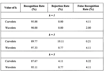
There are three parameters for evaluating the performance of a face recognition

Recognition rate corresponds to the number of correct classification among all the images

tested. The system rejects images in case of a tie or when no common class exists. When

the images are assigned to the wrong class i.e. when Mr. A is wrongly identified as Mr.

B, it is called false recognition. These parameters are usually expressed in terms of

percentage. The results for the three datasets are given in the following page. Few

5.3.1.1 Experiments on Essex Grimace Database

• Image size = 50 x 45

• Train: Test = 8:12

Table 5.1: Curvelet based results for Essex Grimace

Value of k Recognition Rate

(%)

Rejection Rate

(%)

False Recognition Rate

5.3.1.2 Experiments on A T& T Database

• Image size = 56 x 46

• Train: Test = 6:4

Table 5.2: Curvelet based results for AT&T

Value of k Recognition Rate