A Crank–Nicolson collocation spectral method for the two dimensional telegraph equations

R E S E A R C H

Open Access

A Crank–Nicolson collocation spectral

method for the two-dimensional

telegraph equations

Yanjie Zhou

_{and Zhendong Luo}

*_{Correspondence:}

[email protected]

2_{School of Mathematics and}

Physics, North China Electric Power University, Beijing, China Full list of author information is available at the end of the article

Abstract

In this paper, we mainly focus to study the Crank–Nicolson collocation spectral method for two-dimensional (2D) telegraph equations. For this purpose, we first establish a Crank–Nicolson collocation spectral model based on the Chebyshev polynomials for the 2D telegraph equations. We then discuss the existence, uniqueness, stability, and convergence of the Crank–Nicolson collocation spectral numerical solutions. Finally, we use two sets of numerical examples to verify the validity of theoretical analysis. This implies that the Crank–Nicolson collocation spectral model is very effective for solving the 2D telegraph equations.

MSC: 65N30; 65N12; 65M15

Keywords: Crank–Nicolson collocation spectral method; Telegraph equation; Existence, stability, and convergence; Numerical experiment

1 Introduction

Because any bounded closed domain inR2 _{can be approximately filled with several} rectangles [ai,bi]×[ci,di] (i= 1, 2, . . . ,I), for convenience and without losing universality, we just assume that= [a,b]×[c,d]⊂R2_{with boundary∂and consider the following} two-dimensional (2D) telegraph equations:

⎧ ⎪ ⎪ ⎨ ⎪ ⎪ ⎩

utt–μu+αut+βu=f(x,y,t), (x,y,t)∈×[0,T],

u(x,y,t) =ϕ(x,y,t), (x,y,t)∈∂×[0,T],

u(x,y, 0) =H(x,y), ut(x,y, 0) =G(x,y), (x,y)∈,

(1)

whereuis the unknown function,utt=∂2u/∂t2,=∂2/∂x2+∂2/∂y2is the Laplace opera-tor,T is the final time,f(x,y,t),ϕ(x,y,t),H(x,y), andG(x,y) are four given functions, and μ= (LCˆ)–1_{,α=GRμ, andβ= (RC}ˆ_{+GL)μare three known positive constants becauseGis} the conductance of the dielectric material,Ris the distributed resistance of the conductor,

Lis the distributed inductance, andCˆ is the capacitance between the two conductors. For convenience, but without losing generality, we further assume thatϕ(x,y,t) = 0.

The telegraph equations have a very significant physical background, so that they have become a type of important evolution partial differential equations (PDEs) and have been

successfully used in many numerical simulations in mathematical and physical problems used to describe the propagation of an electric signal in a cable of transmission line and wave phenomena. Especially, they can be suitable for modeling the interaction between reaction and diffusion in physics and biology (see [1,2]). Therefore, the study for the tele-graph equations has significant meaning. However, the teletele-graph equations in the real-world problems usually include the complex known data, such as the complicated initial and boundary value conditions, the intricate source term, the discontinuous coefficients, so that they have no analytic solution. Thus we have to rely on numerical solutions.

The finite difference scheme (FDS), the finite element method (FEM), the finite volume element method (FVEM), and the spectral method are regarded to be four most popular methods, but the accuracy of the spectral method is highest in the four numerical meth-ods because it adopts smooth functions (such as trigonometric functions, Chebyshev’s polynomials, Jacobi’s polynomials, and Legendre’s polynomials) to approximate unknown function, whereas FEM and FVEM usually adopt standard polynomials to approximate an unknown function, and FDS adopts difference quotient to approximate derivative. Par-ticularly, with rapid development of computers, the spectral method has achieved great success in many numerical computing fields (see, e.g., [3,4]). The spectral method is a weighted residual way for PDEs and generally is classified as the Galerkin spectral method, the spectral tau method, and the collocation spectral (CS) method, which are used to solve many PDEs including the second-order elliptic equations, parabolic equations, hyperbolic equations, and hydromechanics equations (see, e.g., [3–9]).

Although FDS, FEM, and FVEM have been used to solve the telegraph equations (see [1,

2,10–16]), as far as we know, the spectral method, especially the CS method, has yet not been used to solve the 2D telegraph equations. Therefore, in this paper, we first develop a Crank–Nicolson CS (CNCS) model for the 2D telegraph equations. Then we analyze the existence, uniqueness, stability, and convergence for the CNCS solutions. Finally, we utilize some numerical simulations to verify the validity of theoretical analysis. It shows that the CNCS model is very valid for solving the 2D telegraph equations.

The remaining contents in this paper are scheduled as follows. In Sect.2, we first re-view the spectral-collocation method and some Sobolev spaces. Then, in Sect.3, we build the CNCS model for the 2D telegraph equations and analyze the existence, uniqueness, stability, and convergence of the CNCS solutions. Next, in Sect.4, we use two sets of nu-merical examples to verify that the results of nunu-merical computations are accorded with the theoretical analysis and to certify that the CNCS model is very valid for solving the 2D telegraph equations. Finally, we supply the main conclusions and discussion in Sect.5.

2 The CS method and some useful Sobolev spaces

2.1 The CS method

LetPNbe an interpolation subspace in a one- or two-dimensional space. The CS method consists in that the solution u of PDE is approximated with the interpolation polyno-mialuN inPN, whose interpolation nodes adopt the so-called Chebyshev–Gauss–Lobatto (CGL) points (see [4]).

The Chebyshev polynomials are some special Jacobi polynomials, which are orthogonal with the Chebyshev weight functionω(x) = 1/√1 –x2_{over [–1, 1], namely,}

1

–1

where

γn=Tn2ω=

1

–1

T_n2(x)ω(x) dx.

Let{xj}N_j=0 and{yk}N_k=0 be two sets of space nodes, that is, the CGL points inx andy

directions, respectively, and let{ωk}N_k=0be a set of weights. They are, respectively, defined by

xk= –cos πk

N , yk= –cos kπ

N , ωk=

π

ckN

, 0≤k≤N, (2)

wherec0=cN = 2 andck= 1 (k= 1, 2, . . . ,N– 1). They have the following property (see, e.g., [3]).

Theorem 1 Let {xk}N

k=0, {yk}Nk=0, and{ωk}Nk=0 be the sets of CGL quadrature nodes and

weights,respectively.Then

1

–1 1

–1

p(x,y)ω(x)ω(y) dxdy= N

j=0 N

k=0

p(xj,yk)ωjωk, ∀p(x,y)∈P2N–1. (3)

More specifically, the CS basic principle is to get an approximate solution foru(x,y) by a sum

uN(x,y) = N

j=0 N

k=0

uN(xj,yk)hj(x)hk(y), (4)

whereuN(x,y)∈PN, the interpolation nodes{xj}Nj=0and{yk}Nk=0are the CGL points given by (2), and{hj(x)}_j=0N and{hk(y)}N_j=0are the Lagrange basis polynomials associated with the sets of the CGL points{xj}N

j=0and{yk}Nk=0, respectively. Moreover, the derivative ofuN(x,y) atxkis obtained by

∂uN(xk,y) ∂x =

N

j=0 N

l=0

uN(xj,yl)hj(xk)hl(y), 0≤k≤N, (5)

where the first-order derivativeh_j(xk) at the CGL points can be computed by the following formulas:

h_j(xk) = ⎧ ⎪ ⎪ ⎪ ⎪ ⎪ ⎪ ⎨ ⎪ ⎪ ⎪ ⎪ ⎪ ⎪ ⎩

–2N₆2+1, k=j= 0, ck

cj

(–1)k+j

xk–xj , k=j, 0≤k,j≤N,

– xk

2(1–x2_k), 1≤k=j≤N– 1, 2N2₊₁

6 , k=j=N,

(6)

2.2 Some useful Sobolev spaces

First, we supply several useful Sobolev spaces, whose detailed descriptions can be found in [17].

Let∈R2be a bounded open domain with boundary∂, and letL2() denote the set of all square-integrable functions defined on, equipped with inner product and norm

(u,v) =

uvdxdy and u0=

|u|2dxdy

1/2

, ∀u,v∈L2().

For a nonnegative integermandα= (α1,α2) (whereαi≥0 are integers, and|α|=α1+α2), define

Hm() =u∈L2() :Dαu∈L2(), 0≤ |α| ≤m, equipped with norm and seminorm

um=

0≤|α|≤m Dα_u2

0 1/2

and

|u|m=

|α|=m Dαu2₀

1/2 ,

whereDα_u= ∂|α|u

∂xα1∂yα2. SetH0m() ={u∈Hm() :Dαu(x)|∂= 0,|α|<m}and letH–m()

denote the dual space ofHm 0().

Further, letω=:ω(x,y) =ω(x)ω(y) = 1/(1 –x2_{)(1 –y}2_{),= (–1, 1)}2_{, and letL}2

ω()

de-note the set of all square-integrable functions defined on, equipped with norm

u0,ω=

|u|2ωdxdy

1/2 ,

and letHm

ω() :={u∈L2ω() :D α_u∈L2

ω(), 0≤ |α| ≤m}be the weighted Sobolev space

onwith the CGL quadrature weight function, equipped with the norm

um,ω=

0≤|α|≤m

Dαu2_0,ω

1 2

.

Furthermore, letH_0,1ω() ={u∈Hω1() :u|∂= 0}, (·,·)ωdenote the weighted inter product

ofL2ω() =Hω0(), and let · Hl(Hm

ω)be the norm in the space

Hl0,T;H_ωm()≡

v(t)∈H_ωm() :v2_Hl_(Hm ω)≡

T

0 l

i=0 _dd_tiiv(t)

2

m,ω

dt<∞

.

Next, define theHω1-orthogonal projectionRN :H0,1ω()→PN such that, for anyu∈

H1 0,ω(),

∇(RNu–u),∇v

or, equivalently,

uN(x,y) =RNu(x,y) = N

j=0 N

k=0

uN(xj,yk)hj(x)hk(y). (7)

Therefore we can also approximate the unknown solutionu(x,y) withRNu(x,y). Further,

RN has the following important property (see [4, Chapter III]).

Theorem 2 For any u∈Hωq()with q≥1,we have

∇RNu0,ω≤ ∇u0,ω, ∂k(RNu–u)_0,ω≤CNk–q, 0≤k≤q≤N+ 1,

where C is a general positive constant independent of N andt and used subsequently. Finally, we provide several formulas used often in the following discussions.

(1) The Poincaré inequality. There exist a constantCpsuch that

Cpum≤ |u|m≤ um, ∀u∈H₀m().

(2) The Hölder inequality.

|uv|dxdy≤

|u|2dxdy

1

2

|v|2dxdy

1 2

, ∀u,v∈L2().

(3) Green’s formula.

vudxdy= –

∇u· ∇vdxdy+

∂

v∂u

∂nds, ∀u∈H

2_(),∀v∈H1_(),

whereu=∂2_u/∂x2_+∂2_u/∂y2_{,∇u= (∂u/∂x,∂u/∂y), andnis the unit outer normal}

vector on∂.

(4) The Cauchy inequality.

ab≤εa

2

2 +

b2

2ε, ∀a≥0,b≥0,ε> 0.

3 The CNCS method for the 2D telegraph equations

3.1 The analysis of the existence, uniqueness, and stability of weak solutions for the 2D telegraph equations

Since by using transformsx = –1 + 2(x–a)/(b–a) andy = –1 + 2(y–c)/(d–c) we can ensure [a,b]↔[–1, 1] and [c,d]↔[–1, 1], respectively, for convenience, we can assume thata=c= –1 andb=d= 1 in the subsequent discussions. By using Green’s formula we can obtain the following weak form for the 2D telegraph equations (1).

Problem 3 Find u∈H2_(0,T;H1

0,ω())such that

⎧ ⎨ ⎩

(utt,v)ω+μ(∇u,∇v)ω+α(ut,v)ω+β(u,v)ω= (f,v)ω, ∀v∈H_0,1ω(),

u(x,y, 0) =H(x,y), ut(x,y, 0) =G(x,y), (x,y)∈.

In the following, we employ the variational principle (see, e.g., [3,4]), and the Hölder and Cauchy inequalities to analyze the existence, uniqueness, and stability of the weak solution for Problem3. We have the following main conclusion.

Theorem 4 If f ∈L2_(0,T;L2

ω()),G∈L2ω(),and H∈Hω1(),then there exists a unique

generalized solution u∈H2_(0,T;H1

0,ω())for the variational formulation(8)satisfying the

following stability: ut0,ω+u1,ω≤ ˜C

G0,ω+H1,ω+fL2_(H–1 ω )

, (9)

whereC˜ = 2max{1,β, 1/(2α)}/min{μ,β}.

Proof Because (8) is equivalent to (1) and the system of equations (1) has a generalized solutionuof other form, just as obtained in [10], which is a solution in (8), it is only nec-essary to demonstrate the uniqueness. Thus, we only need to prove that equation (8) has only a zero solution whenf(x,y,t) =H(x,y) =G(x,y) = 0.

Takingv=utin the first formula of equation (8), we have dut20,ω

2 dt +μ

d∇u2_0,ω

2 dt +αut

2 0,ω+β

du2_0,ω

2 dt = (f,ut)ω. (10)

By integrating (10) from 0 to t∈[0,T] and by the Hölder and Cauchy inequalities we obtain

ut2_0,ω+μ∇u20,ω+ 2α

t

0

ut20,ωdt+βu20,ω

=G2_0,ω+∇H20,ω+βH20,ω+ 2

t

0

(f,ut)ωdt

≤ G2_0,ω+∇H_0,2_ω+βH2_0,ω+ 1 2α

t

0

f2_0,ωdt+ 2α t

0

ut20,ωdt. (11)

Therefore, when f(x,y,t) =H(x,y) =G(x,y) = 0, we obtainu0,ω=∇u0,ω= 0, which

impliesu= 0, that is, equation (8) has a unique weak solutionu∈H1

0,ω(). Further, from

(11) we obtain (9). This completes the proof of Theorem4.

3.2 The CNCS method for the 2D telegraph equations

3.2.1 The establishment of the CNCS model

To establish the CNCS model for the 2D telegraph equations, it is necessary to discretize

uttandutby means of the second-order difference quotient and spatial variables by means of the CNCS method. For this purpose, let{xj}N

j=0and{yk}Nk=0be the space nodes inxand

ydirections, respectively, with

xj= –cos

jπ

N, yk= –cos kπ

N,

un_,u

twith (un+1–un–1)/(2t),uttwith (un+1– 2un+un–1)/t2, andun(x,y) withunN(x,y), namely,

un(x,y)≈un_N(x,y) = N j=0 N k=0

un_N(xj,yk)hj(x)hk(y), 0≤n≤K.

Thus, we can establish the following CNCS model for the 2D telegraph equations.

Problem 5 Find un

N∈UN ≡H0,1ω()∩PN such that ⎧ ⎪ ⎪ ⎪ ⎪ ⎪ ⎨ ⎪ ⎪ ⎪ ⎪ ⎪ ⎩

(un+1_N – 2un_N +un–1_N ,vN)ω+μt

2

2 (∇u n+1

N +∇un–1N ,∇vN)ω

+α₂t(un+1_N –un–1_N ,vN)ω+βt

2

2 (u n+1

N +un–1N ,vN)ω

=t2_(f(t

n),vN)ω, ∀vN∈UN, 1≤n≤K– 1,

u0_N(x,y) =RNG(x,y), u1N(x,y) =u0N+ 2tRNH(x,y), (x,y)∈,

(12)

where f(tn) =f(x,y,tn).

3.2.2 The analysis of the existence,uniqueness,and stability of the CNCS solutions

We further employ the Lax–Milgram theorem (see, e.g., [3]) and the Hölder and Cauchy inequalities to analyze the existence, uniqueness, and stability for the CNCS solutions. We have the following main conclusion.

Theorem 6 If f∈L2(0,T;L2ω()),G∈Hω1(),and H∈Hω1(),then there exists a unique

sequence of solutions un_N ∈UN (n= 1, 2, . . . ,K)for the CNCS model(12)satisfying the

fol-lowing stability: un_N1,ω≤

_{8 +μC}2 p+β

C2

pmin{μ,β} 1/2

∇H0,ω+∇G0,ω

+

t

αmin{μ,β} n

j=1

f(tj)2_0,ω 1/2

, n= 1, 2, . . . ,K. (13)

Proof SetA(u,v) = (u,v)ω+μt

2

2 (∇u,∇v)ω+

αt

2 (u,v)ω+

βt2

2 (u,v)ωandF(v) =t2(f(tn),

v)ω+ (2un_N–un–1_N ,v)ω–μt

2

2 (∇u n–1

N ,∇v)ω+α₂t(un–1_N ,v)ω–βt

2

2 (u n–1

N ,v)ω. Then Problem5

can be rewritten as the following:

Problem 7 Find un_N∈UN ≡H0,1ω()∩PN such that ⎧

⎨ ⎩

A(un+1

N ,vN)ω=F(vN)ω, ∀vN∈UN, 1≤n≤K– 1,

u0_N(x,y) =RNG(x,y), u1N(x,y) =u0N+ 2tRNH(x,y), (x,y)∈.

(14)

It is obvious thatA(·,·) is a bounded and positive definite bilinear functional onUN and, for givenf(tn),un

N, andun–1N ,F(·) is a bounded linear functional onUN. Thus, by the Lax– Milgram theorem (see, e.g., [3]) Problem7has a unique sequence of solutionsun

By takingvN =un+1N –un–1N in the first equation of (14), with the Hölder and Cauchy inequalities, we have

un+1_N –un_N2_0,ω–un_N–un–1_N 2_0,ω+μt 2

2 ∇u n+1

N

2 0,ω–∇u

n–1 N

2 0,ω

+αt 2 u

n+1 N –un–1N

2 0,ω+

βt2 2 u

n+1 N

2 0,ω–u

n–1 N

2 0,ω

=t2f(tn),un+1_N –un–1_{N 0,ω}

≤t3 2α f(tn)

2 0,ω+

αt

2 u n+1 N –un–1N

2

0,ω. (15)

From (15) we obtain

un+1_N –un_N2_0,ω–un_N–un–1_N 2_0,ω

+μt 2

2 ∇u n+1 N

2

0,ω–∇u

n–1

N

2 0,ω

+βt

2

2 u n+1 N

2 0,ω–u

n–1 N

2 0,ω

≤t3 2α f(tn)

2

0,ω. (16)

Summing (16) from 1 tonand using the second formula of (14), we obtain un+1_N –un_N2_0,ω+μt

2

2 ∇u n+1 N

2

0,ω+∇u

n N

2 0,ω

+βt

2

2 u n+1

N

2 0,ω+u

n N

2 0,ω

≤u1_N–u0_N2_0,ω+μt 2

2 ∇u 1 N

2

0,ω+∇u

0 N

2 0,ω

+βt 2

2 u 1 N

2 0,ω+u

0 N

2 0,ω

+t

3

2α n

j=1

f(tj)2_0,ω

≤4t2

C2 p

∇RNH20,ω+

μt2

2

∇RNH20,ω+∇RNG20,ω

+βt 2

2C2 P

∇RNH20,ω+∇RNG20,ω

+t

3

2α n

j=1

f(tj)2_0,ω

≤

4t2 C2

p

+μt 2

2 + βt2

2C_P2 ∇H

2

0,ω+∇G20,ω

+t 3

2α n

j=1

f(tj)2_0,ω, n= 1, 2, . . . ,K– 1. (17)

Thus from (17) we obtain∇un_Nω=un_Nω= 0 (n= 1, . . . ,K) when H(x,y) =G(x,y) =

f(x,y,t) = 0, which impliesun_N= 0 (n= 1, 2, . . . ,K). In other words, the CNCS model (14) has a unique series of solutions. From (17) we immediately attain (13). This completes the proof of Theorem6.

3.2.3 The analysis of convergence of the CNCS solutions

Theorem 8 Under the conditions of Theorem6,the errors between the solution for Prob-lem3and the series of solutions of Problem5have the following estimates:

_{u(tn) –u}n

N1,ω≤C

t2+N–2, 1≤n≤K, (18)

where C is a general positive constant independent to N andt.

Proof Ifut is approximated with (un+1–un–1)/2tandutt is approximated with (un+1– 2un_+un–1_)/t2_{, then we obtain the following semidiscretized formulation of equation (8)} in time: ⎧ ⎪ ⎪ ⎨ ⎪ ⎪ ⎩

(un+1– 2un_+un–1_,v)

ω+μt

2

2 (∇u

n+1_+∇un–1_,∇v)

ω+α₂t(un+1–un–1,v)ω

+β₂t2(un+1_+un–1_,v)

ω=t2(f(tn),v)ω, ∀v∈U, 1≤n≤K– 1,

u0(x,y) =G(x,y), u1(x,y) =H(x,y), (x,y)∈,

(19)

Leten₁=u(tn) –un_,en

2=un–RNun, anden3=RNun–unN.

(1) First, estimateen 1.

At timet=tn, by applying Taylor’s expansion to (8) and subtracting (19), taking

v=en+1

1 –en–11 , using Green’s formula and the Hölder and Cauchy inequalities, we

obtain

en+1₁ –en₁2_0,ω–en₁–en–1₁ 2_0,ω+μt 2

2 ∇e n+1 1

2 0,ω–∇e

n–1 1

2 0,ω

+αten+1₁ –en–1₁ 2_0,ω+βt2en+1₁ 2_0,ω–en–1₁ 2_0,ω

=t 4

12

utttt

ξ₁n,en+1₁ –en–1_{1 ω}–μt 4

2

utt

ξ₂n,en+1₁ –en–1_{1 ω}

+αt 4

6

uttt

ξ₃n,en+1₁ –en_1ω+βt 4

2

utt

ξ₂n,en+1₁ –en–1_{1 ω}

≤αten+1₁ –en–1₁ 2_0,ω+ t 7

144αutttt

ξ₁n2_0,ω+μ 2_t7 4α utt

ξ₂n2_0,ω

+αt 7

36 uttt

ξ₃n2_0,ω+β 2_t7

4α utt

ξ₂n2_0,ω, (20)

wheretn≤ξ1n,ξ2n,ξ3n≤tn+1. Becausee11=e01= 0, simplifying and summing (20) from 1ton, we obtain

2en+1₁ –en₁2_0,ω+t2∇en+1₁ 2_0,ω+∇en₁2_0,ω+ 2βt2e₁n+12_0,ω+en₁2_0,ω

≤C2(u)min{μ, 2β}t6, (21)

where

C2(u) = 1

72αmin{μ, 2β}utttt

ξ₁n2 0,ω+ 18μ

2_u tt

ξ₂n2

0,ω

+ 4α2uttt

ξ₃n2 0,ω+ 36β

2_u tt

ξ₂n2

0,ω

Further, we obtain

en_11,ω≤C(u)t2. (22)

(2) Next, estimatee2.

The estimate ofe2can be immediately obtained by Theorem2, that is, when

un_∈H3_(),

en_21,ω≤CN–2, n= 1, 2, . . . ,K. (23)

(3) Finally, estimatee3=RNun–unN.

Subtracting Problem5from (19) takingv=vN∈UN, we obtain

un+1–un+1_N – 2un–un_N+un–1–un–1_N ,vN

ω

+μt 2

2

∇un+1–un+1_N +∇un–1–un–1_N ,∇vN

ω

+αt 2

un+1–un+1_N –un–1–un–1_N ,vN

ω

+βt 2

2

un+1–un+1_N +un–1–un–1_N ,vN

ω

= 0, ∀vN∈UN, (24)

By Theorem2, (24), the property ofRN, the Hölder and Cauchy inequalities, and

Taylor’s formula we have

en+1₃ –en₃2_0,ω–en₃–en–1₃ 2_0,ω+μt 2

2 ∇e n+1 3

2 0,ω–∇e

n–1 3

2 0,ω

+αt 2 e

n+1 3 –en–13

2

0,ω+βt

2_en+1 3

2 0,ω–e

n–1 3

2 0,ω

=un+1– 2un+un–1–un+1_N – 2un_N+un–1_N ,en+1₃ –en–1_{3 ω}

+RNun+1–un+1– 2

RNun–un

+RNun–1–un–1

,en+1₃ –en–1_{3 ω}

+μt 2

2

∇un+1–un+1_N +∇un–1–un–1_N ,∇en+1₃ –en–1_{3 ω}

+μt 2

2

∇RNun+1–un+1

+∇RNun–1–un–1

,∇en+1₃ –en–1_{3 ω}

+βt 2

2

un+1–un+1_N +un–1–un–1_N ,en+1₃ –en–1_{3 ω}

+βt 2

2

RNun+1–un+1+RNun–1–un–1,en+13 –en–13

ω

=RNun+1–un+1– 2

RNun–un

+RNun–1–un–1

,en+1₃ –en–1_{3 ω}

+βt 2

2

RNun+1–un+1+RNun–1–un–1,en+13 –en–13

ω

≤αt 2 e

n+1 3 –en–13

2

0,ω+Ct

Becausee1

3=e03= 0, summing (25) from1ton, we get en+1₃ –en₃2_0,ω+μt

2

2 ∇e n+1 3

2 0,ω+∇e

n 3

2 0,ω

+βt2en+1₃ 2_0,ω+en₃2_0,ω

≤Ct2N–4, n= 1, 2, . . . ,K. (26)

Thus we obtain

en_31,ω≤CN–2, n= 1, 2, . . . ,K. (27)

By combining (22)–(23) with (27) we get (18). This completes the proof of

Theorem8.

Remark1 Theorems6shows that in the CNCS model, that is, Problem5, for the 2D tele-graph equations, there exists a unique series of the solutions that is stable and continuously depends on the initial value and source functions. In order that the error estimates in The-orem8attain an optimal order, it is necessary to take the time-steptandNsatisfying tN–1_{. This theoretically ensures that Problem5is effective and reliable for solving} the 2D telegraph equations.

4 Numerical experiments

In this section, we utilize two sets of numerical experiments to verify the correction of the theoretical results of the CNCS model, that is, Problem5, for the 2D telegraph equations. These numerical examples are implemented by Matlab software in Laptop (Microsoft Sur-face Book: Int Core i7 Processor, 16 GB RAM).

4.1 Example 1

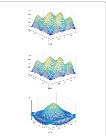
In the 2D telegraph equation (1), we take¯ = [–1, 1]×[–1, 1];L=Cˆ =R=G= 1, that is,α= 1,β= 2,μ= 1;ϕ(±1,y,t) = (1 –cos2πy)exp(–t) (–1≤y≤1 andt∈[0,∞)),ϕ(x,±1,t) = (1 –cos2πx)exp(–t) (–1≤x≤1 andt∈[0,∞)),H(x,y) = 1 –cos2πxcos2πy,G(x,y) = cos2πxcos2πy– 1, andf(x,y,t) = 3exp(–t) + (8π2– 3)cos2πxcos2πyexp(–t). Thus we can find the following analytical solutions for the telegraph equations (1):

u(x,y,t) = (1 –cos2πxcos2πy)exp(–t), (x,y,t)∈[–1, 1]×[–1, 1]×(0,∞).

When we take the time stept= 0.01 and the number of nodes in every directionN= 100, from Theorem8, the theoretical errors between the analytical solution and the CNCS solutionsun

N (n= 1, 2, . . . ,K) should beO(10–4).

Figure 1 (a)The CNCS solution whent= 0.0.(b)The analytical solution whent= 0.0.(c)The errors between the analytical solution and CNCS solution att= 0.0

because both errors are not greater thanO(10–4_{). This implies that the CNCS model is} efficient and feasible for solving the 2D telegraph equations.

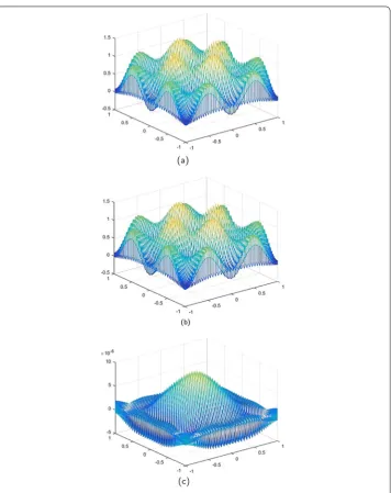
4.2 Example 2

In the 2D telegraph equation (1), we still took¯ = [–1, 1]×[–1, 1];L=Cˆ =R=G= 1, that is, α = 1, β = 2, μ= 1; ϕ(±1,y,t) = 0 (–1≤y≤1 and t∈[0,∞)), ϕ(x,±1,t) = –sinπxexp(0.5t) (–1≤x≤1 andt∈[0,∞)),H(x,y) =sinπxcosπy,G(x,y) = 0.5sinπx×

cosπy, andf(x,y,t) = (2.75 + 2π2_{)sinπxcosπyexp(0.5t). Thus we can find the following} analytical solutions for the telegraph equations (1):

Figure 2 (a)The CNCS solution whent= 0.3.(b)The analytical solution whent= 0.3.(c)The errors between the analytical solution and CNCS solution att= 0.3

When we take the time stept= 0.01 and the number of nodes in every directionN= 100, by Theorem8the theoretical errors between the analytical solution and the CNCS solutionsun

N (n= 1, 2, . . . ,K) still isO(10–4).

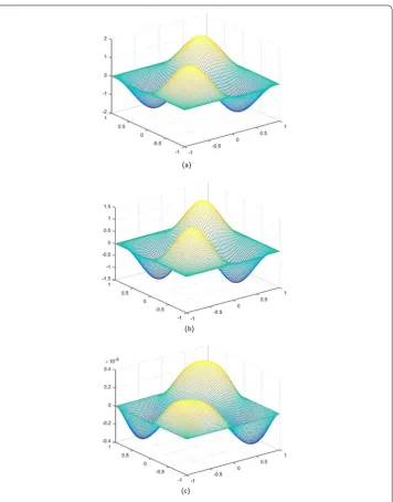
Figure 3 (a)The CNCS solution whent= 0.5.(b)The analytical solution whent= 0.5.(c)The errors between the analytical solution and CNCS solution att= 0.5

Remark2 The accuracy of the CNCS solutions is far higher than other numerical meth-ods, for example, the time–space FEM. For instance, in [10], though the time step is taken as 0.0025 and the space step is taken as 0.0000625, the accuracy of the time–space FEM solutions only attains 10–3_{, whereas our time-step is only 0.01 andN= 100, or,} equiva-lently, the space step is also taken as 0.01, but the accuracy of the CNCS solutions can attain 10–6_.

5 Conclusions and discussion

Figure 4 (a)The CNCS solution whent= 0.9.(b)The analytical solution whent= 0.9.(c)The errors between the analytical solution and CNCS solution att= 0.9

to check the feasibility and effectiveness of the CNCS model and to verity that the numer-ical computing consequences accord with the theoretnumer-ical ones. Moreover, we have shown that the CNCS model is very valid for solving the 2D telegraph equations.

Even if we only study the CNCS method for the 2D telegraph equations, the CNCS method can be easily and effectively used to solve for the telegraph equations in the three-dimensional space or the telegraph equations with complex geometric domains.

for-Figure 5 (a)The CNCS solution whent= 0.9.(b)The analytical solution whent= 0.9.(c)The errors between the analytical solution and CNCS solution att= 0.9

mat with very few unknowns in other paper, so that it can greatly lessen the accumulation of the rounding errors.

Acknowledgements

The authors are thankful to the honorable reviewers and Editors for their valuable suggestions and comments, which improved the paper.

Funding

This research was supported by the National Science Foundation of China grants 41704047 and 11671106, the National Key Research and Development Project of China Grant 2017YFC1500301, and the cultivation fund of the National Natural and Social Science Foundations in BTBU Grant LKJJ2016-22.

Availability of data and materials

Competing interests

The authors declare that they have no competing interests.

Authors’ contributions

Both authors contributed equally and significantly in writing this article. Both authors wrote, read and approved the final manuscript.

Author details

1_{School of Science, Beijing Technology and Business University, Beijing, China.}2_{School of Mathematics and Physics,}

North China Electric Power University, Beijing, China.

Publisher’s Note

Springer Nature remains neutral with regard to jurisdictional claims in published maps and institutional affiliations.

Received: 17 February 2018 Accepted: 8 June 2018

References

1. Hesameddini, E., Asadolahifard, E.: A new spectral Galerkin method for solving the two dimensional hyperbolic telegraph equation. Comput. Math. Appl.72, 1926–1942 (2016)

2. Mittal, R.C., Bhatia, R.: A collocation method for numerical solution of hyperbolic telegraph equation with Neumann boundary conditions. Int. J. Comput. Math.2014, 1–9 (2014)

3. Guo, B.Y.: Spectral Methods and Their Applications. World Scientific, Singapore (1998)

4. Shen, J., Tang, T.: Spectral and High-Order Methods with Applications. Science Press, Beijing (2006)

5. Luo, Z.D., Jin, S.J.: A reduced-order extrapolation spectral-finite difference scheme based on the POD method for 2D second-order hyperbolic equations. Math. Model. Anal.22(5), 569–586 (2017)

6. An, J., Luo, Z.D., Li, H., Sun, P.: Reduced-order extrapolation spectral-finite difference scheme based on POD method and error estimation for three-dimensional parabolic equation. Front. Math. China10(5), 1025–1040 (2015) 7. Guo, B.Y.: Some progress in spectral methods. Sci. China Math.56(12), 2411–2438 (2013)

8. Baltensperger, R., Trummer, M.R.: Spectral differencing with a twist. SIAM J. Sci. Comput.24, 1465–1487 (2003) 9. Canuto, C., Hussaini, M.Y., Quarteroni, A., Zang, T.A.: Spectral Methods in Fluid Dynamics. Springer, Berlin (2012) 10. He, S., Li, H.: Time discontinuous space-time finite element method for telegraph equations. Appl. Math. J. Chin. Univ.

Ser. A27(4), 425–438 (2012)

11. Mohanty, R.K.: New unconditionally stable difference schemes for the solution of multi-dimensional telegraphic equations. Int. J. Comput. Math.86(12), 2061–2071 (2009)

12. Hashemi, M.S., Baleanu, D.: Numerical approximation of higher-order time-fractional telegraph equation by using a combination of a geometric approach and method of line. J. Comput. Phys.316, 10–20 (2016)

13. Biazar, J., Eslami, M.: A new method for solving the hyperbolic telegraph equation. Comput. Math. Model.23(4), 519–527 (2012)

14. Ma, W.T., Zhang, B.W., Ma, H.L.: A meshless collocation approach with barycentric rational interpolation for two-dimensional hyperbolic telegraph equation. Appl. Math. Comput.279, 236–248 (2016)

15. Elgindy, K.T.: Higher-order numerical solution of second-order one-dimensional hyperbolic telegraph equation using a shifted Gegenbauer pseudospectral method. Numer. Methods Partial Differ. Equ.32(1), 307–349 (2016)