2016 Joint International Conference on Artificial Intelligence and Computer Engineering (AICE 2016) and International Conference on Network and Communication Security (NCS 2016)
ISBN: 978-1-60595-362-5
Fuel-optimal Lorentz-augmented Spacecraft Formations Using Novelty
Minimum Sliding Mode Error Feedback Controller
Si-Zhen LU
1,a, Cao LU
2,b, Xiao-Yan ZHANG
2,c, Xiao-Yong QIN
2,d,*1College of Computer Science, Sichuan University, Chengdu, Sichuan, China
2State Key Laboratory of Astronautic Dynamics, Xi'an Satellite Control Center, Xi'an, Shaanxi, China a[email protected], b[email protected], c[email protected],
*Corresponding author
Keywords: Spacecraft Formation Flying (SFF), Minimum Sliding Mode Error Feedback Control (MSMEFC), Nonsingular Terminal Sliding Model Control (NTSMC), Lorentz Spacecraft, Geomagnetic Lorentz Force.
Abstract. A dynamics model of satellite formation flying (SFF) is derived in an elliptical orbit with the existence of J2 perturbation and the Lorentz force. The Lorentz force is considered as the propellantless electromagnetic propulsion for orbital maneuvering and maintenance. However, the direction of Lorentz force is limited by the local magnetic field and the velocity of the spacecraft with respect to the local magnetic field, which is unable to provide the required control acceleration timely; therefore, it always works as an auxiliary strategy to reduce the fuel consumptions. Based on the above assumptions, the fuel-optimal control scheme is proposed for the SFF based on the minimum sliding mode error feedback controller (MSMEFC), which is implemented by using the thruster control and Lorentz force. Moreover, the optimal trajectories of the required specific charge of deputy Lorentz spacecraft and the thruster-generated control acceleration have been developed with details, respectively. Numerical examples are presented to demonstrate the efficacy of the proposed controller to maneuver and maintenance the SFF with the optimal fuel consumptions.
Introduction
According to the fundamental physical principle, a moving charged particle experiences the Lorentz force in a magnetic field. It is deduced that a charged spacecraft could actively generate the Lorentz force by modulating its surface charge when it moves through the Earth’s magnetic field. Therefore, the Lorentz force is a possible good means to control the spacecraft without the fuel consumptions [1-2]. However, due to the limitations that the directions of Lorentz force is determined by the local magnetic field and the velocity of the spacecraft with respect to the local magnetic field. As the result of this constrain, the Lorentz force cannot completely replace the traditional propulsion technologies. It always works as a means of auxiliary propulsion to reduce the expenditure of the fuel onboard, which can extend the work life and reduce the life cycle costs for the most space missions [3-4]. Thus, the concept of Lorentz-augmented spacecraft has attracted the enough attentions and become the hot research spot, since it is proposed [5-7].
perform the orbital control. The work life cycle of most SFF missions are constrained by the amount of propellant onboard, especially for the deputy spacecraft to maneuver or maintenance with respect to the chief spacecraft for a long time. It is anticipated that the formation flight is one of the important applications for which the Lorentz-augmented orbits is well suited. Yamakawa et al. studied the effect of the Lorentz force on the relative motion between spacecraft [19]. Shu et al. discussed the control problem for the SFF by using the Geomagnetic Lorentz force in a circular or elliptical orbit [12]. The optimal Lorentz-augmented controller had been proposed for the SFF in elliptic orbits by Xu [3]. Pollock et al. studied the relative motion, which includes the effect of both Lorentz and coulomb forces [20].
Obviously, the developments of the SFF technology by using the Lorentz force have the important theoretical values and broad application prospects. However, due to the characteristics of SFF technology and the physical properties of Lorentz force, its development poses tremendous challenges. The main challenge is to control the relative position between the chief and deputies in the formation when the external perturbations from gravitational perturbation, atmospheric drag, solar radiation pressure, and Earth oblateness cause the drifts of desired formation position [17]. Additionally, the Lorentz force is constrained by its directions in the Earth’s magnetic field. The optimal combined strategy between the Lorentz force and thruster force is the theoretical difficulty to address. With a view to tackle these challenges, this paper focuses on developing the robust control schemes with the Lorentz force that can achieve the formation objectives, even in the presence of unknown spacecraft masses, uncertainties and perturbations.
In this paper, a novelty controller is proposed based on the minimum sliding mode error feedback control (MSMEFC) with the optimal use of the Lorentz force for SFF. The MSMEFC is first proposed by Cao et.al [21-22], which is a robust nonlinear feedback sliding mode control (SMC) methodology with the advantages of rapid response, even to estimate the external perturbations. Hence, the novel revision of MSMEFC is innovative developed by three steps. The first step is to design an adaptive nonsingular terminal SMC (ANTSMC) with the estimation of spacecraft masses without the effects of unknown perturbations. Based on the controller designed in the first step, a cost function is formulated on the basis of the principle of minimum sliding mode error; then the unknown perturbations are estimated and fed back to the ANTSMC, which constitutes the new MSMEFC. It is obvious that the new MSMEFC can estimate the spacecraft masses and unknown perturbations, in order to enhance the control performance and precisions. Then, to minimize the fuel consumption of the new MSMEFC for SFF, the optimal control law of Lorentz force is proposed as the auxiliary propulsion by solving the fuel-optimal objective function [17].
The present paper is organized as follows. Section.2 introduces the complete nonlinear mathematical model of the SFF system and deduces the Lorentz force experienced by a charged spacecraft. The novelty MSMEFC is formulated with the optimal Lorentz force as the auxiliary propulsion, which is demonstrated with detailed proof of stability in the presence of unknown spacecraft mass, thruster fault and external perturbations in Sec.3. For a detailed assessment of the proposed control strategy, numerical simulations are performed in Sec.4 to verify its effectiveness. In Sec.5, some discussions and concluding remarks are presented.
Dynamic Model of Spacecraft Formation Flying Equation of Relative Motion
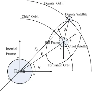
The investigated system comprises a chief spacecraft in an elliptical planar trajectory and a deputy spacecraft moving in a desired relative trajectory around the chief, as shown in Fig.1. The inertial coordinate systemOXYZis attached to the center of the Earth. The chief orbit is described by a radial
distance
,0,0
T 3 c rc r from the center of the Earth, which is under the J2influence and the true
local-vertical-local-horizontal (LVLH) frame as Fig.1. The relative orbit position vector ρ is expressed in this frame. Hence, the relative position and velocity of the deputy satellite from the origin of the chief satellite coordinate frame is defined by , 3,
, ,
T,
, ,
Tx y z x y z
ρ ρ ρ ρ ,
respectively.
c
r
d
[image:3.612.221.377.132.288.2]r
Figure 1. Illustration of a chief-deputy type of satellite formation.
In this study, the spacecraft are modeled as point masses and theJ2perturbations of the chief and
deputy spacecraft are considered in the mathematical model. Hence, the relative motion for the chief spacecraft with respect to the deputy, taking into account the thrust, Lorentz force and perturbation forces, can be written in the form of TH equations [23].
0
2 0
2 2 c c c
c c
r r + r
r r
. (1)
Whereis the instantaneous angular rate of the chief orbit and is the acceleration of true anomaly.
2
2 2
3
2
2 2
3
2 2
3
2 2
2
dx cx cx Lx x c
dy cy cy Ly y c
dz cz cz Lz z c
x y y x x J J a a d
r
y x x y y J J a a d
r
z z J J a a d
r
. (2)
Wherejc d, for the chief spacecraft and deputy spacecraft, respectively. is the gravitational
constant of the Earth. J d a a2, , ,L care the accelerations due to theJ2gravitational potential, disturbance
force, Lorentz force and thruster control force, respectively.
To obtain the relative acceleration arising in the presence of theJ2effects, the method proposed by
Schweighart and Sedwick [24] is used. The relative acceleration vector is obtained by multiplying the relative position vector by the gradient of theJ2potential field.
2 2d 2c 2 rc
Where theJ2gradient is given by:
2 2 2
2
2 2 2
2
2 5
2 2
1 3sin sin sin sin 2 sin 2 sin
6 1 1 7 1
sin sin 2 sin sin sin 2 cos
4 2 4 4
1 3 1 5
sin 2 sin sin 2 cos sin sin
4 4 2 4
e c
c
i i i
J R
r i i i
r
i i i
J . (4)
The gradient can be simplified by orbit-averaging it to capture only the secular effects and eliminate the periodic effects. To obtain that simplified version, the following integral is used:
2
2 0 2 3
2 2 2
4 0 0
1
0 0
2
0 0 3
3 8 1 3cos 2
c e c s d s r s
s J R r i
J J. (5)
Inserting into Eq.(2) and rearranging the terms yields:
2
3 3
2
3 3
3 3
2 2 4
2 3 Ux x c c Uy y c c Uz z c c
x y y s x a d
r r
y x x s y a d
r r
z s z a d
r r
. (6)
Where aU acaL. For the convenience of the controller design and the estimation of spacecraft
mass, the Eq.(6) can be restated as:
D D d
m ρm AρBρ U F t . (7)
2 3 3 2 3 3 3 3 ,2 4 0
0 2 0
0 , 2 0 0
0 0 0
0 0 3
D u d D
c c
c c
c c
m t m t
s r r s r r s r r
U a F d
A B
. (8)
WheremD stands for the unknown mass of deputy spacecraft,
3 1
, , T
x y z
u u u
U is the total
control force of the thruster and Lorentz force. It is assumed that the control input has the saturation limit defined by N uj N j, x y z, , .
3 1
, , T
d Fdx Fdy Fdz
F is the external disturbance forces on the
Lorentz Force
In this subsection, the acceleration of Lorentz force is derived by a particle of chargeqin the
rotating reference. The chief spacecraft is assumed to fly in a given elliptical orbit with the inclination anglei. Let
X Y Z, ,
be an ECI reference frame whose origin is at the center of the Earth, wheretheX axis points towards the vernal equinox andZ axis is towards the North Pole, theY axis
completes the right-hand triad. To simplify the analysis, assume that the geomagnetic field can be modeled as that of a perfect dipole at the center of the Earth and the magnetic North Pole is aligned with the Earth’s geographic North Pole. In terms of the spherical coordinates, which consist of radiusr, colatitude angle, and azimuth fromXaxis, the magnetic field can be expressed as:
0
3 2cos ˆ sin ˆ 0ˆ B
r
B r . (9)
Where B0 is the strength of the field in weber-kilometer. Then the Lorentz
accelerationaLexperienced by a particle with chargeqmoving through a magnetic fieldBis given by:
L rel e
q q
m m
a V B V ω r B. (10)
Where q m is the specific charge (i.e., charge-to-mass ratio) of Lorentz spacecraft,
withqandmbeing the charge and the mass of the Lorentz spacecraft, respectively. Vreldenotes the
relative velocity of the Lorentz spacecraft with respect to the local magnetic fieldB. Vis the velocity vector of the spacecraft and theωeis the Earth’s angular velocity vector. Hence, the Eq. (10) shows
that the rotation of the magnetic field allows the Lorentz force to do work on the spacecraft.
One first needs to expressVrelin terms of the Hill coordinates. The detailed explanations of the
coordinate transformation leading to the expression ofVrelin the Hill frame is provided in reference
[26]. The expression for the Lorentz spacecraft’s velocity relative to the local magnetic field is given:
cos cos sin
cos sin sin
cos sin sin sin
c e e
x
rel y c e e
z c e e
x r y i z i
V
V y r x i z i
V z r x i y i
V
. (11)
Then, letrin the ECI frame
X Y Z, ,
coordinate system ber
X Y Z
T. Thusrˆ, , ˆ ˆin Eq. (9) are given by:
2 2 2 2
2 2
1 ˆ 1 1
ˆ , , ˆ
0
X XZ Y
Y YZ X
r r X Y X Y
Z X Y
r . (12)
Where 2 2 2
r X Y Z . Then the magnetic fieldBin Eq.(9) is given by:
0 5
2 2 2
3 3 2
x y z
XZ B
B
YZ B
r
B
Z X Y
To obtainBin the Hill frame, all the quantities appearing on the right hand side of Eq. (13) must be expressed in the Hill frame. The absolute position vectorr rc ρ
rcx
, ,y zTis obtained in the Hillframe as:
3 1 3
R R R
c
i c i i
i c i i
i c i i
X r x
Y i y
Z z
X c c s c s r x c s s c c y s s z Y s c c c s r x c c c s s y c s z Z s s r x c s y c z
. (14)
3 1 3
cos sin 0 1 0 0 cos sin 0
R sin cos 0 , R 0 cos sin , R sin cos 0
0 0 1 0 sin cos 0 0 1
i i i
i i
. (15)
Where c and s denote the sine and cosine functions of the angle given as subscript. Hereis the right ascension of the ascending node and iis the inclination angle of the chief spacecraft.
Based on the above discussions, the Lorenz accelerations expressed in RM frame can be formulated by substituting Eq. (11) and Eq. (13) into Eq. (10) as:
, ,
T
L x y z
x y z z y y z x x z z x y y x
l l l
l V B V B l V B V B l V B V B
a l
. (16)
In the present investigations, the desired trajectory is calculated from the circular formation. The chief and deputy spacecraft keep a constant separation from each other, and the formation model is
mathematically defined as 2 2 2 2
dc
x y z r . The equations of the desired circular trajectory are given as
follows:
sin 2cos 2
3 sin
d dc d d
x nt
r
y nt
z nt
. (17)
Where rdcis the circular formation size, is the phase angle between the chief and the deputy
satellite (the initial phase angle is determined through the initial conditions), andnis the mean orbital
rate of the chief trajectory. In this paper, we only deal with this kind of formation type, although the proposed controller developed is applicable to any formation types and spacecraft configurations.
Novelty MSMEFC Design with Lorentz Force
Based on the chief-deputy SFF mathematical model presented in the previous section, we present the theoretical basis for developing the novelty MSMEFC with the optimal Lorentz force for the SFF in the presence of unknown spacecraft masses, thruster fault and external disturbances. The design of proposed MSMEFC can be divided into three parts [21-22], which is given with details in the following parts.
To facilitate the discussions below, we define the relative state vector and the desired relative trajectory asρ ρ,and , 3
d d
ρ ρ , respectively. The performance index are defined as the tacking errorε ε, 3.
,
d d
As discussed earlier, the deputy spacecraft massmDis assumed to be unknown. It is estimated
online by the proposed adaptation law that provides the estimate parameter to the controller. Therefore, the parameter estimation error is given by:
ˆ
D D D
m t m m t . (19)
WheremˆD
t denotes the estimate of the deputy spacecraft massmD. For the closed-loop system,the estimated parameter does not converge to their true value; therefore, the parameter update law is only introduced for the robustness purpose [17].
Basic Controller for Novelty MSMEFC
The first step of the novelty MSMEFC is to derive the basic controller for SFF without the external disturbances based on the ANTSMC. It is well known that the control performance of a SMC relies heavily on the chosen sliding manifold. The ANTSMC owns the nonlinear hyper-plane-based sliding mode, which has a wide variety of design strategies with rapid and finite time convergence [26].
Based on the SFF system described by Eq. (7) and the definition of the tracking error in Eq.(18), the nonsingular sliding manifold is designed as
1 1
p q C
S ε ε . (20)
Where 3 3
1
C is a constant, strictly positive, diagonal matrix. The positive odd
integerspandqsatisfy the following condition:
pq. (21)
It is important to pay attentions that one of the vectors has the fractional power in the nonlinear sliding surface in Eq.(20). For the vectorεp q, the fractional power is defined as.
The ANTSMC design starts with building sliding manifold in the system state space. Our objective is to derive the control law that can drive the deputy spacecraft to a desired trajectory and maintain it there. Therefore, we derive the control law to estimate the deputy spacecraft mass, which is given based on the Lyapunov stability theorem without considering the effects of the external disturbances. The candidate Lyapunov function is defined as follows [17, 26].
2
1 1
1
1 1
2 2
T
D D
m m
V S S . (22)
Where1is a positive constant. Taking the derivative ofValong its trajectory gives:
1
1 1 1 1
1 1
1
1 1
1
1 ˆ 1 ˆ
1 ˆ
T T p q
D D D D D D D
T p q
D D D d D D
p
m m m m C m m m
q p
m C m m m m
q
V S S S ε ε ε
S ε ε ρ ρ
. (23)
Substituting formDρfrom Eq.(7), one can obtain:
1
1 1
1
1 ˆ
T p q
D D D d D D
p
m C m m m m
q
Adding the relationship ofmDdescribed in Eq.(19), the new form ofVis as follows:
1 1 1 1 1 1 1ˆ ˆ ˆ
1 ˆ
T p q
D D D d
T p q
D d D D
p
m C m m
q p
m C m m
q
V S ε ε Aρ Bρ u ρ
S ε ε Aρ Bρ ρ
. (25)
It is important to emphasize that the control forceuis different from theUin Eq. (7), which is the process controller without the external disturbances. Based on Eq. (25), the control law described by control force and the adaptive law for the mass of the deputy spacecraft are defined as:
1 2 1
1
1 1 1 1
ˆ , 1 ˆ , 2 p q
eq v eq D d
T p q
v D d
q m C p p m C q
u u u u Aρ Bρ ε ρ
u S S ε ε Aρ Bρ ρ
. (26)
The acceleration form of the control force (26) can be rewritten as:
1 2 1
1
1 1 1 1
,
1 ˆ ˆ
, ,
2
p q
u ueq v ueq d
T p q
v D D d
q C p
p
m m C
q
a a a a Aρ Bρ ε ρ
a S S ε ε Aρ Bρ ρ
. (27)
Where 3 3
, ,
x y z diag
for all
i: i0
, and is similar to.It is important to note that εp q13 3 is a diagonal matrix with the form as follows:
1
1
11 ([ p q p q p q ])
p q
x dx y dy z dz
diag
ε ρ ρ ρ ρ ρ ρ . (28)
Because p and q are positive odd integers, in order to convenient for the control law designed by
Eq. (26) to avoid singular problem, we must add another constrain 1 p 2
q
.
For the SFF mathematical model in Eq.(7), if the basic control law is defined by Eq.(26), then the system will asymptotically approach to the sliding mode surfaceS1
t 0without considering theexternal disturbances. Furthermore, the system tracking errorρ ρ,will converge to zero in finite time.
Estimation of Disturbances for Novelty MSMEFC
Based on the above controller, the external disturbance accelerations are taken into account and the linear sliding manifold is given as follows:
2 C2
S ε ε. (29)
WhereC2
is a constant.
For the high precision control, one hopes that the sliding mode manifold should satisfy
20
For this purpose, we can first expand S2in a Taylor series based on Eq. (27), such that:
2 t t 2 t , , t t , ,t u dC2 d
S S Z ρ ρ Λ V ρ ρ a ρ ρ . (30)
The details aboutZ
ρ ρ, , t
andΛ
t V
ρ ρ, , t
can be found in the references [21-22], which is notdiscussed here for simplicity.
When the system remains in the prescribed sliding manifold, the sliding manifold is called the ideal sliding mode and the corresponding control acceleration isaueq. The Taylor series of the sliding mode
is given by:
2 t t 2 t , , t t , ,t ueq dC2 d
S S Z ρ ρ Λ V ρ ρ a ρ ρ . (31)
Therefore, a new evaluation criterion is described, which is the error covariance between the actual sliding mode and the ideal sliding mode, such that:
2 2 2 2 , , , ,
T T T T
v v
t t t t t t t t t t t t
R S S S S Λ V ρ ρ a a V ρ ρ Λ . (32)
For compensating the effects of disturbances on the actual control accelerationaU, the unknown
disturbances accelerationd
t is introduced and the actual control acceleration is modified by:,
U u ueq v ueq v u U ueq v
a a d a a d a a a a d a a d. (33)
Insertingauinto Eq. (30) and rearranging this term yields the Taylor series of the sliding mode with
the feedback of the unknown external disturbances. The sliding mode is defined as estimated sliding mode, such that:
2 2 2
2 2
, , , ,
, , , , , ,
u d d
U d d
t t t t t t C
t t t t t t C
S S Z ρ ρ Λ V ρ ρ a ρ ρ
S Z ρ ρ Λ V ρ ρ a Λ V ρ ρ d ρ ρ
. (34)
In order to achieve the optimal unknown disturbances, it is assumed that the consistent estimates of the unknown disturbances must match the following relationship. The residual error covariance between the estimated sliding modeSˆ2
t and the ideal sliding modeS2
t approximates equivalent tothe known error covariance between the actual sliding modeS2
t and the ideal sliding modeS2
t .The necessary condition is hereafter called the “minimum sliding mode covariance constraint” [21]. The covariance constraint is required to satisfy the following approximation:
2 2 2 2
ˆ ˆ T
t t t t t t t t
S S S S R. (35)
Therefore, the estimated sliding manifold Sˆ2
t t
is required to approach the ideal slidingmodeS2
t t
with approximately the same error covariance as the ideal sliding mode fits the actualsliding modeS2
t t
. A cost function to estimate the unknown disturbances is defined as:
1
2 2 2 2
1 ˆ ˆ 1
2 2
T
T
t t t t t t t t t t t
J d S S R S S d Wd . (36)
unknown disturbance acceleration to be added should be minimized. The optimal disturbances should be adjusted by a minimal amount.
Substituting from Eq. (34) and minimizing Eq. (36) with respect to unknown disturbances accelerationd , such that:
1
1 1
2 2
T T
ueq d d
t C
d ΛV R ΛV W ΛV R S Z ΛVa ρ ρ . (37)
According to the second order system Eq.(7), some intermediate variables can be derived, such that:
2
2
2 3 3 2 2
1 1
, , , , ,
2 2
t t t t C t t t C tC
Λ V ρ ρ I Z ρ ρ Aρ Bρ ρ. (38)
Therefore, the control law described by control force in Eq.(26) is modified as follows:
1 2 1 1 1 1 1 2 2 11 1 1
1 ˆ , , 2 ˆ ˆ p q
eq v d eq D d v
T T
d D ueq d d
T p q
D d q m C p m C p m C q
U u u F u Aρ Bρ ε ρ u S
F ΛV R ΛV W ΛV R S Z ΛVa ρ ρ
S ε ε Aρ Bρ ρ
. (39)
The corresponding control acceleration in Eq. (27) can be expressed as:
1 2 1 1 1 1 1 2 2 11 1 1
1 ˆ
, , ,
2
ˆ
p q
U ueq v ueq d v D
T T
ueq d d
T p q
D d q C m p C p m C q
a a a d a Aρ Bρ ε ρ a S
d ΛV R ΛV W ΛV R S Z ΛVa ρ ρ
S ε ε Aρ Bρ ρ
. (40)
The stability proof of this controller is given in Ref [22].
Fuel-Optimal Lorentz Force for Novelty MSMEFC
To achieve SFF, the deputy spacecraft thrusts continuously to fix its position relative to the chief spacecraft to satisfy the desired position. Based on the analysis in the previous studies, the Lorentz acceleration is almost impossible to provide the required acceleration for SFF at any instant. For most cases, the Lorentz acceleration could only work as the auxiliary propulsion to cooperate the thrusters on board, which is also used to reduce the fuel consumption.
Therefore, if the control acceleration is made up of two parts asaU acaL, the ac is the control
acceleration generated by the thruster on board and theaLis the Lorentz acceleration for the fuel
saving. To minimize the fuel consumption for SFF, following fuel-optimal objective function is considered as [4].
0 , 0 0
T T T T T
a
L t t dt
c cdt
U U dtJ a a a l a l . (41)
WhereTrefers to the orbital period of the chief.
Solving the Euler-Lagrange equation as follows:
0
d L L
dt
Yields the fuel optimal specific charge of Lorentz spacecraft for SFF, as:
2 00 0
U
l a l l
l
. (43)
Hence, the optimal thruster-generated control acceleration is obtained as:
2 0
0
U U c
U
a l
a l l
a l
l a
. (44)
Furthermore, the optimal thruster-generated control force can be computed by multiply the Eq. (44) with the deputy spacecraft mass. In addition, the near-term feasible maximum of the specific charge is assumed to about0.3C kg, which is larger than many published papers. Hence, the required specific
charge has the limitation as 0.3C kg. It is obvious that the novelty MSMEFC is developed and
implemented by the combination Eq.(39) or (40) with Eqs.(43) and (44), which can satisfy the control requirements of SFF with fuel-optimal Lorentz force in the presence of unknown spacecraft mass, thruster fault and external disturbances.
Simulation Results
To study the effectiveness and performance of the proposed novelty MSMEFC with fuel-optimal Lorentz force, the sufficient numerical examples are simulated by using the equations of motion (7) for SFF with the proposed controller (26) and (43). The desired formation is given by Eq.Error! Reference source not found. for the circular formation in elliptical orbit. The performance evaluation presented in this section is divided into two subcategories. First, the effectiveness of the controller for a fault-free case of SFF is given with details and analyzes the fuel consumption with the estimation of unknown disturbances and mass of spacecraft. Then, we examine the effects of thruster degradation, thruster stuck fault and short-term thruster failure on the performance of the proposed control strategies.
For all the simulations presented in this section, the unknown disturbance forceFd
t acting on theSFF system is assumed to be time varying, which incorporates atmospheric drag, solar radiation pressure, and some unknown perturbations from the internal or external of the spacecraft. In order to shown the performance of the proposed controller, the unknown disturbances model is deliberately magnified and given by:
3
1 1.5sin 1.5 10 0.5sin 2
sin
dx dy dz
F nt
F nt N
F nt
. (45)
Wherenis the mean angular velocity and equal to 3 c a
( is the gravitational parameter of the Earth and acis the semi-major axis of the chief spacecraft). The SFF system parameters and its orbital
[image:11.612.141.471.687.719.2]parameters for the chief satellite are shown in Table 1. The control parameters used in all simulations for the novelty MSMEFC are shown in Table.2.
Table 1. Orbital and system parameters.
Parameter m kg, , 3 2
e km s
,
p
r km e i, deg ,deg , ,M,deg
Table 2. Controller parameters for numerical simulation.
Parameter C i1i
1,2,3
C i2i
1,2,3
p q,
1 W ii
1,2,3
i
i1, 2,3
N ii
1,2,3 ,
mNMSMEF 100 5 {11,9} 0.02 105 0.1 10
In this subsection, the simulation results are given and analyzed for the fault-free case of SFF. The desired formation structure considered is a projected circular formation, described by Eq. (17) with 1km formation radius. The phase anglebetween the chief and deputy spacecraft is assumed to be20. The initial states for numerical simulation are computed by substituting t0in Eq. (17) and adding a
1km position offset on three directions. The initial velocity components for all states are calculated by taking the time derivative of Eq. (17) and substituting t0. The initial conditions for mass estimates
and the initial conditions for formation are given as follows:
0 1 0.5 2 0 1 ; ˆD
0 9X m . (46)
In order to assess the effectiveness of the proposed methodologies completely, the control cost can be employed as another important criterion. The value of a spacecraft always lies on its life span, and the life fuel span always depends on the fuel left. Therefore, a controller based on less fuel consumption will always be preferable. Hence, we adopt the following mathematical model to calculate the control cost required for SFF:
2 2 2
0 t
cx cy cz
Energy
u u u dt. (47)Where, uci,ix y z, , is the control thrust for SFF, which can be employed as a measure of fuel
consumption.
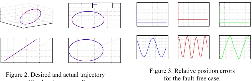
The simulation results are shown for the fault-free case in Figs 2-5 when there is a 1km position offset on all three relative states. The objective is to stabilize the formation when there an initial misalignment exists. It is clear that the proposed novelty MSMEFC shows its advantages in the position error convergence in Fig 2-3. The estimate of unknown disturbances and mass are simulated in Fig.4. It is manifest that the estimated disturbances will have some severe fluctuations in the initial phase. Due to the sliding mode error covarianceRError! Reference source not found. cannot match match the weighting matrixW at the beginning; the unknown disturbances cannot be estimated accurately. With the control precision improved gradually, the sliding mode error covarianceRcan match the weighting matrixW well; therefore, the estimated disturbances can reflect the actual disturbances accurately. In addition, the dynamic coupling of x y, directions in Eq. (7) strengthen the
estimated performance ofFdxand Fdy; thus, the estimated result inz direction has a little weak
performance in Fig.4. For the estimation of the mass of spacecraft, the estimated error is less than 2%, which can fully show the effectiveness of the proposed method.
Figure 2. Desired and actual trajectory of the deputy spacecraft.
[image:12.612.89.531.576.718.2]
[image:13.612.197.411.66.173.2]
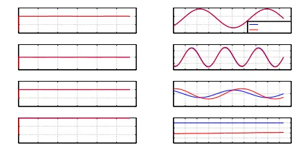
Figure 4. The estimate of unknown disturbances and mass of the spacecraft.
[image:13.612.115.526.206.357.2]
Figure 5. Thrust demand control force for the uncharged and charged spacecraft.
Figure 6. The specific charge of deputy spacecraft and energy comparisons of
uncharged and charged spacecraft. Although a 1km position offset is very high and the control force is saturated at 10mN, the control forces are saturated quickly in the short period with high control precision in Figs. 3 and 6. With the auxiliary Lorentz force, the thruster control force of charged spacecraft is slighter than that of uncharged spacecraft. To modify the serious initial position offset, the deputy spacecraft needs large control force, most of which is provided by the thruster on-board. Because, the auxiliary Lorentz force is limited by the directions of the local magnetic field and velocity, which cannot generate enough Lorentz force for the three directions at any time with the limitation of the maximum specific charge. But it can also reduce the fuel consumption with time accumulated in Fig.6. It is obvious that the charged spacecraft can save the fuel on-board over than that of uncharged spacecraft for the formation keeping with optimal specific charge.
Conclusions
References
[1] M. Peck, Prospects and challenges for Lorentz-augmented orbits. AIAA Guidance, Navigation and Control Conference, AIAA, Reston, VA, AIAA Paper 2005, 2005, pp: 15-18.
[2] B. Streetman, M. Peck, New synchronous orbits using the Geomagnetic Lorentz Force. Journal of Guidance, Control, and Dynamics, 30(2007) 1677-1690.
[3] H. Xu, Y. Ye, Z. Yang, Optimal Lorentz-augmented spacecraft formation flying in elliptic orbits. Acta Astronautica. 111(2015) 37-47.
[4] H. Xu, Y. Ye, Z. Yang et al. Sliding mode control for Lorentz-augmented spacecraft hovering around elliptic orbits. Acta Astronautica, 103(2014) 257-268.
[5] B. Streetman, M. Peck, Gravity-assist maneuvers augmented by the Lorentz force. Journal of Guidance, Control, and Dynamics, 32(2009) 1639-1647.
[6] J. Gangestad, G. Pollock, J. Longuski. Propellantless Stationkeeping at Enceladus via the electromagnetic Lorentz force. Journal of Guidance, Control, and Dynamics, 32(2009) 1466-1475. [7] B. Streetman, M. Peck, General Bang-bang control method for Lorentz augmented orbits. Journal of Spacecraft and Rockets, 47(2010) 484-492.
[8] G.E. Pollock, J.W. Gangestad, J.W. Longuski, Analytical solutions for the relative motion of spacecraft subject to Lorentz-force perturbations. Acta Astronautica, 68(2011) 204-217.
[9] H. Xu, Y. Yan, Z. Yang, Improved analytical solutions for relative motion of Lorentz spacecraft with application to navigation in low Earth orbit. Proc. Inst, Mech. Eng. Part G J. Aerosp. Eng. 228(2014) 2138-2154.
[10] J. Atchison, M. Peck, Lorentz-augmented Jovian orbit insertion. Journal of Guidance, Control, and Dynamics, 32(2009) 1639-1647.
[11] H. Xu, Y. Yan, Z. Yang, Dynamics and control of spacecraft hovering using the geomagnetic Lorentz force. Adv. Space. Res. 53(2014) 518-513.
[12] T. Shu, B. Mai, Y. Hiroshi, Spacecraft formation flying dynamics and control using the geomagnetic Lorentz force. Journal of Guidance, Control, and Dynamics, 36(2013) 136-148.
[13] C. Peng, Y. Gao, Lorentz-force-perturbed orbits with application to J2-invariant formation. Acta Astronaut. 77 (2012) 12-28.
[14] M.A. Peck, B. Streetman, C.M. Saaj, et al. Spacecraft formation flying using Lorentz forces. J. Br. Interplanet. Soc. 60(2007) 263-276.
[15] S.P. Neeck, T.J. Magner, G.E. Paules, NASA’s small satellite missions for Earth observation. Acta Astronautica. 56(2005) 187-192.
[16] R. Kristiansen, P.J. Nicklasson, Spacecraft formation flying: a review and new results on state feedback control. Acta Astronautica, 65(2009) 1537-1552.
[17] G. Godard, K.D. Kumar. Fault tolerant reconfigurable satellite formations using adaptive variable structure techniques. Journal of Guidance, Control, and Dynamics, 33(2010) 969-984. [18] F. Bauer, J. Bristow, J. Carpenter, et al. Enabling spacecraft formation flying in any earth orbit through spaceborne GPS and enhanced autonomy technologies. Space Technology, 20(2001) 175-185.
[20] G.E. Pollock, J.W. Gangestad, J.M. Longuski, Charged spacecraft formations: A trade study on Coulomb and Lorentz forces. Proceedings of the AAS/AIAA Astrodynamics Specialist Conference, (2009) AAS 09-389.
[21] L. Cao, X.Q. Chen, A.K. Misra, Minimum sliding mode error feedback control for fault tolerant reconfigurable satellite formations with J2 perturbations. Acta Astronautica. 96(2014) 201-216. [22] L. Cao, X.L. Li, X.Q. Chen, et al. Minimum sliding mode error feedback control for fault tolerant small satellite attitude control. Advances in Space Research. 53 (2014) 309-324.
[23] T. Carter, Optimal impulsive space trajectories based on linear equations. Journal of Optimization Theory and Applications. 70(1991) 277-297.
[24] S.A. Schweigart, R.J., Sedwick, High-fidelity linearized model for satellite formation flight. Journal of Guidance, Control and Dynamics, 25(2002) 1073-1080.
[25]D.A. Vallado, Fundamentals of Astrodynamics and Applications, Third Edition, Hawthorne, CA: Microcosm Press. 1998.