(will be inserted by the editor)
Effort Estimation of FLOSS Projects: A Study of the Linux
Kernel
Andrea Capiluppi · Daniel Izquierdo-Cort´azar
Received: date / Accepted: date
Abstract Empirical research on Free/Libre/Open Source Software (FLOSS) has shown
that developers tend to cluster around two main roles: “core” contributors differ from “peripheral” developers in terms of a larger number of responsibilities and a higher productivity pattern. A further, cross-cutting characterization of developers could be achievd by associating developers with “time slots”, and different patterns of activ-ity and effort could be associated to such slots. Such analysis, if replicated, could be used not only to compare different FLOSS communities, and to evaluate their stabil-ity and maturstabil-ity, but also to determine within projects, how the effort is distributed in a given period, and to estimate future needs with respect to key points in the software life-cycle (e.g., major releases).
This study analyses the activity patterns within the Linux kernel project, at first focusing on the overall distribution of effort and activity within weeks and days; then, dividing each day into three 8-hour time slots, and focusing on effort and ac-tivity around major releases. Such analyses have the objective of evaluating effort, productivity and types of activity globally and around major releases. They enable a comparison of these releases and patterns of effort and activities with traditional software products and processes, and in turn, the identification of company-driven projects (i.e., working mainly during office hours) among FLOSS endeavors.
The results of this research show that, overall, the effort within the Linux kernel community is constant (albeit at different levels) throughout the week, signalling the need of updated estimation models, different from those used in traditional 9am-5pm, Monday to Friday commercial companies. It also becomes evident that the activity before a release is vastly different from after a release, and that the changes show an
Dr A. Capiluppi
University of East London, UK E-mail: [email protected]
D. Izquierdo-Cort´azar
increase in code complexity in specific time slots (notably in the late night hours), which will later require additional maintenance efforts.
1 Introduction
Software development productivity measurement and cost estimation has been a re-search topic for more than 3 decades [1], [2], [3]. So far, the vast majority of empiri-cal studies have involved data from proprietary software projects [4]. Even though an increasing number of governments, non-governmental organizations and companies seem interested in using, evaluating and contributing to FLOSS, effort estimation models or other measurement-based models are not generally used within FLOSS communities [4]. Indeed, such exploration and quantification of productivity, specif-ically the determination of how a FLOSS community manages and allocates effort around a major release, may help in comparing FLOSS projects both with propri-etary software projects, and also be useful when making comparisons between large FLOSS communities. Furthermore, such productivity modeling can also help to iden-tify a baseline to measure the possible impact of changes in, for example, processes, methods and tools used by FLOSS communities.
The analysis of FLOSS productivity so far has shown that there is an increase in productivity as long as FLOSS developers progress in their statuses within a project. A good approximation of such observed practice has been visualised along the clus-ters of the so called “onion model” [5], [6]. The external layer of this representation consists of users, strictly speaking not representing developers, but nonetheless form-ing a valuable community for both the diffusion of FLOSS products and the testform-ing of their functionalities. The contributors, less numerous than the users, represent the next layer, producing source code and fixes, as well as providing feedback and discus-sion. Finally, the core developers, representing the centre of the onion, provide most of the work needed both in the creation, and in the maintenance, of new or existing content, and their productivity is an order of magnitude higher than the contributors. It has been also argued that the core team must be small [7] in number, in order to keep a tight control over the core system. It has also been found that the coordina-tion issues of tradicoordina-tional software systems (e.g., Brooks’ law [8]) still apply within FLOSS core teams, while such issues are much less relevant in other layers of the onion model [9].
The objective of this research is to develop a framework for FLOSS effort es-timation based on clustering developers around different time slots, and by consid-ering “days of the week” or “hours in a day” as cross-cutting attributes for effort and productivity models. The rationale for doing this derives from both a lack of such differentiation in the current literature, and the results obtained in a previous work [10] analysing the effort produced by a UK-based software development com-pany. A Source Code Management system (SCM) is kept by the company1, so daily and weekly analyses are possible: among other results, it was found that the pattern
1 All the developers are co-located, so no further adjustments are needed in terms of the time of the day
of activity could be described by a traditional 9am-to-5pm, Monday to Friday com-mitment. Most days experience comparable effort levels, apart from Thursdays, when most of the “user stories” get completed, and Fridays, when mostly testing is done.
Performing a similar analysis for FLOSS projects could lead to better understand-ing of how the FLOSS development works, and whether its characteristic activity and effort distributions are so different as to render “traditional” effort estimation software cost models unusable. On the one hand, the analysis could highlight productivity pat-terns around specific dates (e.g., when a major release is made public). On the other hand, its results could be used to determine whether specific time slots are more pro-ductive, or are more prone to modifications that increase the code complexity, than others.
In both cases, the wealth of data coming from FLOSS projects could help produce and replicate ad-hoc estimation models, eventually differentiating company-driven projects from community-driven endeavors. FLOSS projects backed by large compa-nies (i.e., company-driven) should reflect developers with a more traditional, 9am-5pm activity patterns, commit policies and so forth. The community-driven FLOSS projects should instead follow more continuous working patterns, since developers are working in their spare time, and outside normal “office hours”. If identified and confirmed, such emerging patterns would present new, specific challenges:
– how to differentiate the effort estimation models based on the periods of activity,
by means of weights and triggers of model-switching; and
– the effective utilization of monitoring tools in specific time intervals, or parts of
the day, in order to properly monitor the diverse productivity at certain times of the day, or in specific days of the week.
So far, this research has achieved four main contributions:
1. It demonstrates that the patterns of work within the selected case study (the Linux kernel) are different from those found in a traditional software development team. 2. It presents the analysis of the development of the Linux kernel along specific pe-riods of the day (e.g., time slots), and in specific pepe-riods (around major releases), with the aim of investigating the changes in productivity and code complexity during such periods.
3. It performes the analysis using the “Git” SCM repository, which offers additional information on the development processes, not offered by other repositories, and not used in previous studies on FLOSS systems. In comparison with other config-uration management systems (such as CVS or SVN), a Git repository retains the information about both the authors and their local submission dates, rather than aggregating the latter into the central server’s time [11]. With this information, it is possible to group the developers’ effort based on the effective time of the day when such actions were performed. This provides valuable information when a distributed, trans-national development approach is considered (as the FLOSS model requires).
2 Empirical Approach
This section details the various steps of the empirical process to extract the met-rics and the results from raw data, given a number of research questions, for the purpose of allowing other researchers to replicate the steps for other FLOSS (but not only) systems. One of the contributions of this paper is in terms of the method and a baseline that can be used for comparison with other systems. The section is articulated as follows: subsection 2.1 introduces the basic terminology and the def-initions used throughout this study; subsection 2.2 illustrates the research goal and questions, together with the metrics used to accomplish such goal, using the GQM framework [12]; subsection 2.3 details the process used to obtain the selected met-rics, using the history logs contained within the Git repository of the Linux kernel; subsection 2.4 finally illustrates the process and tools used to extract the complexity metric of the single source files, and of all the revisions that each file underwent.
2.1 Definitions
The definitions used in the following study are as follows:
– Commit (or revision): change on the source code submitted to the source code
management system. This updates the current version of the tree directory with a new set of changes. Those changes are generally summarized in a patch which is a set of lines with specific information about the affected files, but also about the affected lines. In this paper, the link between amount of commits and developers’ effort is established from previous literature [13].
– Committer: any person with rights to commit a change into the source code. – Author: At times, a commit is committed by a given committer, but she may not
be the real (or only) author. Some SCMs offers this information, and the Git SCM provides a specific field for this.
– Major release: this research will focus on specific points when higher activity
is detected, namely the releases of the Linux were made publicly available. The releases studied in this research are the ones contained (or migrated) within the Git repository during the 2.6 branch of development, starting from release 2.6.12 and including release 2.6.34. In total, an overall of 23 releases were analysed, spanning some 5 years of development under the Git repository.
– Timezones: in this research any day is divided into three 8-hour sections, with
“office hours” (OH) defined as the period from 9:00 to 17:00 between Mondays and Fridays; similarly “after office” (AO) is the period from 17:00 to 1:00, and “late night” (LN) runs from 1:00 to 9:00. As mentioned above, and differently from other systems (e.g., CVS, Subversion), the Git configuration management system records and permanently stores the times local to the individual commit-ter, which makes the definition of timezones feasible, and the study of working patterns along different hours of the day possible.
– Complexity: since the Linux kernel is developed mainly using the C
2.2 Goal-Question-Metric Approach and Research Questions
This section presents the general objective of this work, and it does that in the for-mal way proposed by the Goal-Question-Metric (GQM) framework [12]. The GQM approach evaluates whether a goal has been reached, by associating that goal with questions that explain it from an operational point of view, and providing the basis for applying metrics to answer these questions. This study follows this approach by developing, from the wider goal of this research, the necessary questions to address the goal and then determining the metrics necessary for answering the questions.
Goal: the long term goal of this research is to define, validate and update
produc-tivity models for FLOSS projects, and to differentiate them from existing proprietary software models.
Question: In this research, and considering the Linux Kernel as a case study, the
following research questions have been evaluated:
Q1 – Is the effort towards the Linux kernel development evenly distributed?
Rationale: the aim of this question is to compare the distribution of changes in the source code with those provided by the company studied in [10]. This will also provide a first impression of the general distribution of the changes and a first determination of the main differences between fully company-driven project and a partially community-driven and company-driven project such as the Linux Kernel.
Q2 – Do Linux developers work specifically during some days of the week, or some
hours of the day?
Rationale: the aim of this question is to check how the development activity car-ried out by the developers of the project is distribited between the different days of the week.
Q3 – Is there a statistically significant difference in the activity during various parts
of the day?
Rationale: the division of a day in time slots could help to improve the knowledge about the different activities carried out by developers. This is also helpful to develop an estimation model based on which time slots the commercial companies usually work in (termed in this paper, Office Hours - OH) and extend such model to FLOSS projects by adding information from the other time slots (AO and LN).
Q4 – Is there a statistically significant difference in the activity before and after a
major release in the Linux kernel?
Rationale: The aim of this question is to show how developers within the Linux Kernel work around deadlines and release dates. It is known that some FLOSS communities deal with deadlines similarly to software companies, imposing hard dates and “feature-freeze” periods before a deadline [16], [17]. Thus, this ques-tion aims to quantify the pre-release effort and post-release efforts, and it pro-vides an oversight of how the Linux Kernel community deals with these dates of high-load commitment.
Q5 – Are some parts of the day more prone than others to changes that increase the
complexity?
such changes were submitted. From an intuitive point of view, a developer who is performing time-consuming and highly intellectual work such as programming will not be likely work at the same level of concentration during all of the different time slots being studied.
Q6 – What is the relevance of the factor “time slot” for an estimation model?
Rationale: this final question aims to create a first approximation model for the estimation of the effort in FLOSS communities based on the results provided by the Linux Kernel community.
Metrics: For the purpose of this research, it is worth emphasizing again that,
within the Git system, the association of commit times to time slot uses the local time of the developer, not some central timestamp provided by a central repository (as in the CVS and Subsversion systems). Two empirical studies have been carried out in this research, one related to the characterization of the overall activity of commits by committers during the whole development log of the Linux kernel; and the other focused only on the major releases between (and including) 2.6.12 and 2.6.34, and analysing the development activity both one week before, and one week after a major release. For each of the addressed questions a set of metrics have been defined and the empirical approach and method followed as explained in section 2.3 and 2.4:
1. Q1, Q2, Q3: In order to answer these questions, a weekly and hourly commits activity is proposed in the study. In addition, a small study about a randomly selected week has been carried out to study – at the granularity of lines – the dif-ferent types of activity carried out by the developers (added, modified or removed lines).
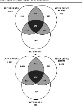
2. Q4: For this question, the metrics extracted are at first the overall activity in num-ber of commits for each of the pre- and post-release periods, and secondly the activity before- and after-releases in each of the different time slots. Each of these series of data was compared before- and after-release using the appropriate hy-pothesis testing (i.e., the Student’s t-test was used). In addition, differentiating between authors and committers, a study about the number of people working in each of the time slots is carried out. These people are divided by unique contrib-utors in the different time slots, intersection of contribcontrib-utors among the different time slots and finally, an intersection with all of the authors and committers that have contributed in the three time slots during their activity period in the commu-nity.
3. Q5: The aim of this question is to look for significant complexity changes in the different time slots, but it is also focused on the different pre- and post-release pe-riods. For this purpose an increase or decrease of the McCabe complexity metrics for each of the files that have been handled in each of the periods and time slots is calculated and analysised.
2.3 Empirical Approach – Overall Activity
The first part of the paper is devoted to the characterization of development activity within the Linux kernel: the following empirical approach was followed in this first part:
1. Git clone: at first, the Linux Git repository2 was cloned and stored locally. As reported above, this repository spans the late life-cycle of the Linux Kernel (since April 2005), when the project was moved to the Git repository.
2. Data pre-parsing: the information contained in the log of such repository was parsed into commonly used results: the CVSAnalY toolset was used for this pur-pose. CVSAnalY has been developed at one of the authors’ institution, and it can be found at the Libresoft tools Git repository3. In terms of functionality, it of-fers more advanced features than other freely availabe tools [18], [19]; in terms of testing, it has been extensively used as the core toolset in a large EU project4. In this research, the toolset was used to save each commit ID, and the relevant data along that commit, including the time, the authors and the committer, and the rationale of such commits.
3. Time and full-path parsing: further to the pre-parsing by the CVSAnalY tool, the time attribute of each commit was clustered in one of three slots, “office hours”, “after office” or “late hours”, depending on the hour of such commit. 4. Major release dates: from the overall activity log of the Linux kernel (obtained
by issuing the “git log” command), the dates of each of the aforementioned re-leases were clearly identified by a “release announcement” statement, and cross-validated, for each release, with the upload date to re-distribution websites (e.g.,
http://www.kernel.org/pub/linux/kernel/v2.6/).
5. Identify commits before and after a release: in order to identify the list of com-mits performed during the seven days before a major release (but excluding the actual day of release), the database produced by CVSAnalY was queried starting from the midnight of the first day, till the 23:59 of the seventh day5.
6. Added, Deleted and Modified lines: each commit is parsed with the ‘diffs-tat’ utility, which uses the more common ‘diff’ program to define summaries of added, deleted and modified lines within a large, complex set of changes. In particular, for each commit, the switch “-m” is used to summarize a large chunk of modifications in a readable format.
7. Authors and Committers: in order to identify the number of committers and au-thors working in each of the aforementioned timeframes and during a pre-release or post-release time, queries on the CVSAnalY database were performed to iden-tify committers and authors working in specific time periods. Authors and com-mitters were first identified for pre-release and post-release periods, and then were further subdivided into those working in specific timeframes (e.g., OH, AO, LN).
2 As found in git://git.kernel.org/pub/scm/linux/kernel/git/torvalds/
linux-2.6.git
3 git.libresoft.es
4 FLOSSMetrics project,www.flossmetrics.org/
2.4 Empirical Approach – Complexity
The second part of this research is devoted to studying whether one of the (or more than one) timezones are more prone to changes that add complexity than other parts of the day. In contrast with the first part of the paper, this second analysis has not produced an overall view of how the complexity is characterized in the whole life-cycle, but it only focuses on the seven days before and the seven after a major release, as defined above.
The following steps were followed to determine how the complexity was intro-duced, increased or reduced along various commits or revisions:
1. Identify files affected in a commit: based on the list of commits executed either before (pre-) or after (post-) a major release, a Git repository gives the opportunity to display all such changes through the “git show” command. The output of such command is used to display a summary of files affected by a revision (say, ’c‘), as in “git show c | diffstat -m”. As a cross-validation of such results, we used the information stored by CVSAnalY in the table “actions”.
2. Extracting the full path of files: Since the basic CVSAnalY only extracts file names, a patched version of such tool was developed in order to extract the full path of the files affected in a specific commit. As a cross-validation of such re-sults, the Git command issued for extracting the full paths of the files affected in a commit ‘c’, is “git show c | diffstat -p1 -w70”.
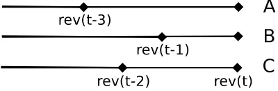
[image:8.595.141.341.481.547.2]3. Evaluating the previous revision of a file: any file in the Git repository, after being added, will go through a series of revisions, ordered by the date when each was performed. If, say, the three files A, B and C were modified in revision rev(t) (Figure 1), each will have a previous revision where they were modified or firstly added (in the example, B in rev(t-1), C in rev(t-2) and A in rev(t-3)). Given a revision ‘r’ of the file ‘f’, the Git repository will show how the file ‘f’ was in that specific revision ‘r’, by issuing the commandgit show r:f. In this way, it is possible to compare two revisions of the same file, and to check whether the changes inputed by a developer affected its structure.
Fig. 1 Evaluating previous revisions of files
so given a revision ‘r’ of the file ‘f’, the formulated command is “git show r:f | pmccabe -F”. By cross-cutting this analysis with the information on the time of each revision, it is possible to conclude whether in any of the time slots developers added or removed complexity, or whether the change left the same complexity unmodified.
3 Results – Development Activity
As mentioned above, the case study is the Linux Kernel which has been previously studied several times and from several points of view ( [20], [21], [22], [23]). Two aspects are presented below: the first considers the whole evolution log of the Linux Kernel (since April 2005, when the overall data has been moved to the Git repository) and it displays the patterns of activity in terms of week-days and hours worked on by the Linux developers (irrespective of them being “core” or “peripheral” developers). The second focuses on specific weeks of the Linux kernel development, justifying this choice with the observed bias in the distribution of effort, and attributed to the presence of major releases.
3.1 Results – Weekly and Hourly Activity
In order to compare and contrast the findings of the activity patterns during working hours and throughout a week of traditionally developed software, the following sec-tion presents the analysis of the Linux kernel development under a similar perspec-tive. As mentioned above, it is possible to reliably extract the “weekly” and (more importantly) the “hourly” activity because of how the Git server stores the informa-tion on the developers activity: the commit date and timestamp of Git uses the local time of the developer, hence recording the time of her activity, rather than imposing the timestamp from a central, shared repository.
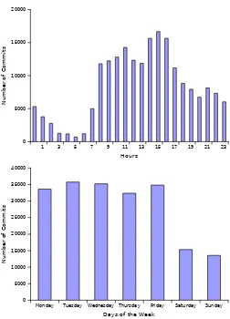
Figure 2 (top) shows the analysis of the overall activity within the Linux Ker-nel during the day, as recorded within the Git log. The first observation is that the work/no-work distinction, found within the commercial counterpart [10], is not eas-ily applicable to the Linux kernel development. The activity performed between 9am and 5pm (corresponding to the “office hours”) accounts for some55%of the overall amount of commits; some31%of the overall activity is produced during the “after work” interval, or between 5pm and 1am; finally, some14%of the activity is per-formed during the “late hours”, or between 1am and 9am. The second and third slots of activity therefore represent a consistent departure from the commercial counterpart studied in [10], reflecting a traditional pattern of activity since most of the commits appear during the “office hours” (Figure 2, left). On the contrary, in the Linux kernel, the most active time slot is found between 2pm and 4pm. Specifically at 3 pm we can see a peak of activity which gradually decreases during the after-office hours.
distribution of activity throughout the week. In this figure, we divide the week in the weekdays and calculate the aggregated number of commits for the whole life of the project. This figure shows how people in the Linux Kernel tend to work during the weekdays: the first, clearly defined period is the interval “Monday - Friday”, where the number of commits is daily more than 30,000. The second period of activity ap-pears specifically during the Saturdays and Sundays, where the number of commits jointly reaches some 30,000 commits (i.e., the same amount of commits achieved in any other day of the week). In summary, the comparison with a traditional com-mercial system shows that the Linux Kernel benefits overall from one “extra” day of development per week (6 days with similar productivity out of 7), whereas the observed commercial system benefits from 5 (unequally productive) days per week.
1 3 5 7 9 11 13 15 17 19 21 23
Hours 0
5000 10000 15000 20000
Number of Commits
Monday Tuesday Wednesday Thursday Friday Saturday Sunday
Days of the Week
0 5000 10000 15000 20000 25000 30000 35000 40000
[image:10.595.115.367.272.622.2]Number of Commits
The observed patterns, in the Linux kernel and in the commercial company, pose an issue of how to quantitatively describe the observed effort, and how to formulate an effort estimation model. Since the distribution of effort is predefined throughout the office hours in a commercial environment, the effort is only applied in that slot: therefore, when expressing the effort as a function of the performed activity (e.g., amount of commits, lines added, modified or deleted; files added, modified or deleted; etc.) the modeled commercial system would need to be modeled by an equation such as
EC(t) =f(activityOH(t)) (1)
whereEC(t)is the development effort in a “commercial” setting during a period t (daily, weekly, monthly, etc), whilef(activityOH(t))is a function of the amount of commits, during the same period, but only within the office hours boundaries (i.e., 9am to 5pm).
On the other hand, when modeling the overall activity seen in the Linux kernel (and most likely other FLOSS systems), and taking into account the three time slots (Office Hours, OH; After Office, AO; Late Hours, LH), one should also take into account the other time slots, and weigh them appropriately:
EF(t) =wOH∗f(activityOH(t))+wAO∗f(activityAO(t))+wLN∗f(activityLH(t)) (2) where whereEF(t)is the development effort in a FLOSS project during a period t (daily, weekly, monthly, etc), wOH is the weight given to the activity observed within the Office Hour slot;wAO the weight to the After Office slot; andwLN the weight to the Late Night slot. In the case of the reported Linux kernel, the overall activity observed in this project, based on the number of commits detected, produce the following weights:wOH= 0.55,wAO= 0.31andwLN = 0.14.
3.2 Results – Types of Activity
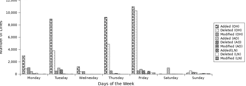
The overall activity shown above has the advantage of proposing the global picture of the development within the Linux kernel, without revealing whether some parts of the day were more prone to specific types of activity (e.g., additions, deletions or modifications). In order to perform a more focused analysis of the type of activity occurring in the various parts of the day, a number of “random” weeks were selected to analyse whether the division of a day in three parts can shed further insights on how work is performed within the Linux kernel.
distribution shown in the previous figures, except for the Wednesday. This seems to be an outlier that does not follow the general tendency in amount of work.
For the mentioned figure, we can observe how the number of lines handled during the weekend (even when we select the whole day and not divided by time slots) is really low, being developed the main activity in this specific week during the week days.
Monday Tuesday Wednesday Thursday Friday Saturday Sunday
Days of the Week 0
2,000 4,000 6,000 8,000 10,000 12,000
Number of Lines
[image:12.595.78.496.189.336.2]Added (OH) Deleted (OH) Modified (OH) Added (AO) Deleted (AO) Modified (AO) Added(LN) Deleted (LN) Modified (LN)
Fig. 3 Size of Changes for the week April 13 - April 19, 2009
In the specific case of the week days, we observe how the quantity of lines (added or removed) in a given day is really high compared to the rest of the day, reaching some days almost the 100% of the total modifications6. On the other hand, we can see how in the weekends, the activity developed by the people (even out of the office time7) is really low, but developed out of the office time. In this case, the activity developed during the weekend reaches up to an 80% on Saturday, and a 40% on Sunday.
Table 1 finally displays, for the aforementioned week, the changes observed, and divides them in three categories: added, deleted and changed lines. As also observed in Figure 3, half of the activity is achieved during the day, in the time slot 9am-5pm, with an overall count of 482 commits.
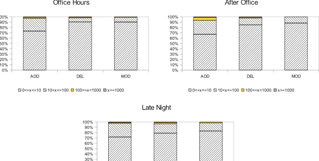
The standard deviation in each slot, the size of the largest commit, and the skew-ness values show that the changes in each time slot have a power law distribution, with up to two changes larger than 1,000 lines per slot. The density distribution of changes (see Figures 4) confirms that some 60-70% of the changes (added, deleted or modified lines) always fall in the size cluster of [0-10] lines. Also in any time slot, and for any type of change (added, deleted or modified lines), more than 95% of such
6 A partial explanation for the low values of activity on April15th
could be that the Federal Income Taxes are due in the United States on that day
7 We provide the results for the office time during the weekends just to observe if there is a continuous
OH :9am−5pm AO :5pm−1am LN :1am−9am
ADD DEL MOD ADD DEL MOD ADD DEL MOD
AVG 36.10 15.80 5.37 40.94 19.45 4.96 95.15 90.32 9.02
STDEV 261.18 208.89 24.97 181.92 154.66 10.77 849.97 848.16 23.03
MAX 3,404 4,542 469 2,244 2,243 95 9,443 9,443 154
[image:13.595.83.404.292.379.2]SKEW 14.38 15.61 11.82 9.11 13.34 5.00 10.99 11.08 4.32
Table 1 Average size of changes, differentiated by time slots and type of change
[image:13.595.85.402.296.456.2]changes are within a [0-100[ lines boundary, while very few changes are over and above 1,000 lines per change, and those are usually coupled to a change of oppo-site sign (e.g., a very large commit of added lines coupled to a very large commit of deleted lines). Although highly skewed, the use of averages to summarise such distri-butions could be considered acceptable, even considering the outliers over and above 1,000 lines.
Fig. 4 Density distribution of changes for the week April 13 - April 19, 2009 – differentiated by time slot
details and analyses the activity observed seven days before and seven days after the date of a major release (while excluding the peak of the release day), for the purpose of producing estimation models based on the types of actions observed in the development.
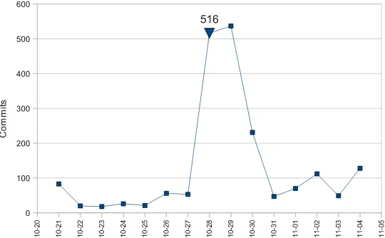
Fig. 5 Activity one week before and one week after the 2.6.14 release
3.3 Results – Before and After a Major Release
The history logs of the Linux kernel contained within the Git repository cover 23 major, from 2.6.12 (inclusive) to 2.6.34 (the latest one studied). Each was analysed with respect to the amount of commits; authors and committers; added, deleted and modified lines as recorded both seven days before, and seven days after the date of each public release.
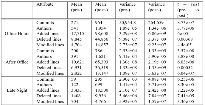
The results of such analysis are reported, as longitudinal trends in the amount of commits per release in Figure 6, and in the tabular form of Table 2, detailing for each studied characteristic, its mean and variance value, both a week before and a week after a major release.
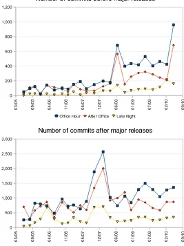
The following findings have been observed:
– The average amount of commits-per-release is somewhat similar during the OH
and AO slots, and both pre- and post- major releases;
– The average amount of commits-per-release during slot LN is clearly lower than
the OH and AO, both pre- and post- major releases, signaling a lower activity in such slot;
– The similarity between the OH and AO slots is consistent for all the studied
Fig. 6 Aggregated commits divided by hour of the day, before (above) and after (below) the major releases
in the Linux kernel
– Despite the lower amount of activity, the Linux kernel had an increasing number
– The distributions of all the measured characteristics were found to be statistically
different, when considering the pre- and post-weeks: for example, the distribution of commits in the OH slot before releases (51, 94, 121, 24, 141, 74, 103, 88, 152, 191, 94, 149, 196, 179, 682, 399, 435, 417, 530, 403, 462, 425, 959) is statistically different from the distribution of commits after releases (258, 269, 824, 797, 739, 484, 963, 722, 766, 631, 884, 1891, 2571, 1018, 739, 1062, 845, 1287, 1498, 1288, 1048, 1272, 1361) when applying the t-test (last column of Table 2,t= 8.73e−07).
Attribute Mean
(pre-)
Mean (post-)
Variance (pre-)
Variance (post-)
t − test
(pre- vs
post-)
Office Hours
Commits 271 964 50,954.8 264,659 8.73e-07
Authors 541 1,954 1.89e+05 1.34e+06 3.77e-06
Added lines 17,715 98,608 3.29e+08 6.86e+09 6e-05 Deleted lines 8,845 44,856 9.08e+07 3.37e+09 0.00368 Modified lines 4,704 14,857 2.73e+07 9.25e+07 4.4e-05
After Office
Commits 200 786 2.53e+04 1.33e+05 3.57e-08
Authors 391 1,621 9.41e+04 5.90e+05 3.88e-08
Added lines 10,621 65,393 1.30e+08 2.19e+09 6.03e-06 Deleted lines 6,931 36,519 1.33e+08 1.35e+09 0.00052 Modified lines 2,822 13,147 1.09e+07 5.63e+07 6.04e-07
Late Night
Commits 59 295 2.90e+03 4.08e+04 6.25e-06
Authors 122 699 1.41e+04 3.71e+05 8.30e-05
[image:16.595.70.414.214.391.2]Added lines 3,433 18,500 2.10e+07 2.42e+08 7.22e-05 Deleted lines 1408 9,936 5.46e+06 7.84e+07 7.41e-05 Modified lines 704 4,766 5.92e+05 1.57e+07 3.36e-05
Table 2 Activity one week before and one week after major releases, clustered by time-slots
Based on such findings, the effort estimation equation in (2), and specifically the term activity(t) should be tailored to reflect such differentiation in both the time slots, and depending on whether the activity is monitored and estimated in the weeks be-fore or after a major release. A list of equations for the activity could be obtained as follows, and based on the assumption that the actions of “adding”, “deleting” and “modifying” lines (or files) are exhaustive of the type of actions perfomed by devel-opers during the period t (say, hourly, daily, weekly, etc):
activityij(t) =wij∗f(Addij(t), Delij(t), M odij(t)) (3)
where i the index indicates whether the activity is observed either “before” or “after” a release; thejindex instead can be used to differentiate between the activity as seen in the OH, AO and LN slots. Thewi
Fig. 7 Intersections of committers (top) and authors (bottom) grouped by time slots
4 Results – Complexity in Time Slots
The third part of this research focuses on the presence of complexity (measured by the McCabe cyclomatic index), and its changes within the source files of the Linux kernel. As reported above, this further study examined the activity:
– of the 23 releases found between April 2005 and June 2010, and
– differentiating the results in “one week before” a release from those “one week
after”, and finally
– clustering each day of activity in the three time-zones: OH, AO and LN.
The analysis was performed only on the “.c” source files and “.h” headers8 that underwent changes during the pre- and post-release weeks. For each of the commits
8 This was done to properly evaluate the McCabe cyclomatic complexity for source files developed in
performed in such weeks, it was studied whether the changes pushed by committers did alter the overall complexity of the affected files. Only the “modified” files were considered in such evaluation, therefore leaving aside the addition of new files (which adds new source code, let aside new complexity). To the best of our knowledge, this is the first time that an analysis of how single source files changed within subsequent commits is performed in a large case study.
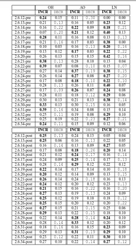
The results are reported in Table 3: they are clustered around the three time slots (OH, AO and LN) and summarized in relative terms. Each time slot presents two series of data, the first (2nd, 4th and 6th columns) depicting the amount of files which underwent an increase of complexity, the second series (3rd, 5th and 7th columns) the amount of files which had a decrease of their overall McCabe cyclomatic number instead: both series are relative numbers, and divided by the amount of files handled in the same week. The following observations were made:
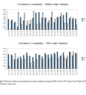
1. During the pre-release weeks, the activity during late night hours has been, so far, the most likely to increase the complexity when modifying the source files. In other words, changes increased file complexity more often in the LN slot than in the OH slot (6 releases out of 23 (70%)). This is also shown in the distribution of such ratios in Figure 8.
2. On the contrary, during the after-release weeks, the Office Hour slot initially seeded more complexity into the source files. In more recent releases, instead both the After Office and the Late Night slots have started to insert more complexity into files, as compared to the Office Hour slot, signaling again the importance of such slots in seeding more complexity within modified files.
3. The distributions of source files undergoing increases of complexity is statistically different in each time slot, when performing a t-test comparison: for instance, the global amount of files undergoing increases of complexity in the OH slot presents statistically relevant differences when comparing the week before9and the week after10a release, when applying the two-tail t-test (1.174E-007).
4. The patterns in the decrease of complexity show instead a different perspective: during the weeks before a release, no major differentiation between the various time slots is visible, each presenting a fluctuating and inconsistent behavior. On the other hand, the after-release weeks show either an overall increase of com-plexity, or a decrease, but not both (as seen in the before-release weeks).
Considering the relation for effort estimation in Equation (2), it is possible to discriminate, within the “activity” term, the portion of such activity devoted to the increase of complexity, the portion that increases the complexity, and the portion that does not affect the complexity. Each of the termsactivityOH(t),activityAO(t)and activityLH(t)can be further expanded in the following:
activityiOH(t) =wOHIC ∗aICOHi (t)+wOHDC∗aDCOHi (t)+wW ChCOH ∗aW ChCOHi (t)
(4)
9 Number of source files where complexity increases, during the week before a release: 13, 33, 28, 1,
48, 33, 30, 48, 54, 87, 36, 37, 72, 56, 190, 149, 129, 128, 237, 216, 177, 146, 314
10 Number of source files where complexity increases, during the week after a release: 100, 102, 256,
OH AO LN
INCR DECR INCR DECR INCR DECR
2.6.12-pre 0.24 0.15 0.11 0.30 0.00 0.00
2.6.13-pre 0.21 0.13 0.16 0.05 0.23 0.12
2.6.14-pre 0.16 0.22 0.22 0.09 0.18 0.21
2.6.15-pre 0.07 0.20 0.21 0.12 0.40 0.13
2.6.16-pre 0.28 0.11 0.16 0.08 0.13 0.13
2.6.17-pre 0.21 0.16 0.17 0.03 0.38 0.00
2.6.18-pre 0.10 0.03 0.16 0.13 0.20 0.16
2.6.19-pre 0.13 0.12 0.17 0.03 0.22 0.22
2.6.20-pre 0.26 0.13 0.15 0.15 0.42 0.16
2.6.21-pre 0.38 0.13 0.28 0.10 0.13 0.04
2.6.22-pre 0.39 0.07 0.08 0.10 0.15 0.07
2.6.23-pre 0.27 0.14 0.37 0.19 0.38 0.15
2.6.24-pre 0.26 0.14 0.27 0.08 0.27 0.20
2.6.25-pre 0.17 0.08 0.18 0.10 0.22 0.10
2.6.26-pre 0.28 0.13 0.26 0.11 0.40 0.07
2.6.27-pre 0.17 0.09 0.26 0.07 0.24 0.08
2.6.28-pre 0.28 0.11 0.18 0.12 0.29 0.06
2.6.29-pre 0.30 0.13 0.21 0.13 0.38 0.14
2.6.30-pre 0.33 0.13 0.30 0.15 0.16 0.05
2.6.31-pre 0.39 0.16 0.34 0.08 0.15 0.14
2.6.32-pre 0.25 0.11 0.19 0.08 0.29 0.10
2.6.33-pre 0.25 0.19 0.22 0.23 0.27 0.21
2.6.34-pre 0.24 0.11 0.15 0.09 0.12 0.06
INCR DECR INCR DECR INCR DECR
2.6.12-post 0.25 0.13 0.24 0.13 0.05 0.04
2.6.13-post 0.25 0.06 0.16 0.13 0.22 0.05
2.6.14-post 0.16 0.14 0.13 0.09 0.27 0.05
2.6.15-post 0.17 0.08 0.18 0.26 0.20 0.14
2.6.16-post 0.21 0.12 0.24 0.17 0.16 0.14
2.6.17-post 0.24 0.09 0.25 0.14 0.17 0.13
2.6.18-post 0.28 0.14 0.29 0.12 0.22 0.12
2.6.19-post 0.22 0.14 0.17 0.14 0.10 0.18
2.6.20-post 0.20 0.12 0.14 0.09 0.13 0.15
2.6.21-post 0.26 0.14 0.24 0.18 0.16 0.13
2.6.22-post 0.24 0.12 0.20 0.12 0.23 0.13
2.6.23-post 0.21 0.15 0.16 0.22 0.16 0.20
2.6.24-post 0.27 0.13 0.19 0.13 0.24 0.09
2.6.25-post 0.25 0.12 0.19 0.10 0.18 0.12
2.6.26-post 0.25 0.15 0.20 0.12 0.20 0.22
2.6.27-post 0.27 0.15 0.21 0.15 0.25 0.06
2.6.28-post 0.29 0.13 0.22 0.15 0.18 0.10
2.6.29-post 0.22 0.14 0.28 0.14 0.24 0.10
2.6.30-post 0.28 0.14 0.33 0.12 0.20 0.12
2.6.31-post 0.18 0.16 0.16 0.15 0.23 0.09
2.6.32-post 0.29 0.13 0.31 0.19 0.29 0.10
2.6.33-post 0.23 0.12 0.22 0.11 0.30 0.10
[image:19.595.95.374.79.584.2]2.6.34-post 0.27 0.10 0.22 0.14 0.27 0.12
Table 3 Percentages of files increasing (i.e., “INCR”) or decreasing (i.e., “DECR”) their complexity,
Fig. 8 Portion of files increasing their overall complexity during Office Time (OT) and at Late Night (LN)
divided by time slots
activityiAO(t) =wAOIC∗aICAOi (t)+wAODC∗aDCAOi (t))+wW ChCAO ∗aW ChCAOi (t)
(5)
activityiLN(t) =wLNIC ∗aICLNi (t) +wLNDC∗aDCLNi (t) +wW ChCLN ∗aW ChCLNi (t)
(6) where wIC
j ,wDCj andwjW ChC are the weights of the activities for increasing (IC), decreasing (DC) or without changes (WChC) in the complexity of the source files during the time slotj. The termsaICi
j(t),aICji(t)andaICji(t)represent the observed activities of increasing, reducing or not affecting the overall complexity of files during during the time slotj, withirepresenting either the week before or after a major release.
aIC aDC aWChC
Pre-week activity
OH 0.24 0.13 0.63
AO 0.21 0.11 0.68
LN 0.24 0.11 0.64
Post-week activity
OH 0.24 0.13 0.64
AO 0.21 0.14 0.64
[image:21.595.86.382.78.159.2]LN 0.20 0.12 0.68
Table 4 Weights to complexity, grouped in time slots and clustered in “before” and “after” a major release
5 Issues of Repeatability
Mining software repositories is a complex task in time, but also in tools and datasets used for retrieving information. Some authors have dealt with the question of repli-cability in software engineering [24], [25]. In addition, Robles [26] has specifically pointed out a number of issues when mining software repositories field. In order to make it possible for other researchers to repeat our analysis, it is necessary to provide availability to raw data, the processed dataset and the available tools or scripts). The overall extraction process has been explained in detail in section 2.3 and 2.4. Thus, this section mostly aims to fill the gaps among the different steps followed in those sections, and to illustrate the results and the scripts or tools used to retrieved them.
– Is the “raw” data publicly available? – The raw data used in this paper is
pub-licly available in the data sources from the Linux Kernel community, and more specifically from the SCM system that can be found at the Git repository. The dates used for this data are the commits available between the dates 2005-04-16 15:20:36 and 2010-06-29 10:42:52 (and consisting of 200,633 commits). The repository can be easily downloaded by means of the git clone command line11.
– Is the processed dataset publicly available? – All the processed data can be
found in a MySQL database format and publicly available 12. This dataset has been obtained using the tools and scripts described in next bullets. All the tables were retrieved by the CVSAnalY tool except: release commits, release dates, compare and changes. With respect to the tables release dates and release commits they were both manually introduced to make the analysis of the data easier, and they were based on data obtained from the distribution website13. While the other two tables contain information automatically retrieved by the use of some scripts specifically created for this purpose.
– Are tools and scripts used in the study publicly available? – The tools and the
scripts used to perform this study are made available, as follows:
– CVSAnalY: This tool can be found at the Libresoft tools Git repository14 and it can be downloaded using the git clone command. The version used in
11 git clone git://git.kernel.org/pub/scm/linux/kernel/git/torvalds/
linux-2.6.git
12 http://mastodon.uel.ac.uk/EMSE2011/cvsanaly_kernel26_git.mysql.zip 13 http://www.kernel.org/pub/linux/kernel/v2.6/
this paper comes from the version found at the master branch on the date of 2010-08-27.
– Scripts: Some scripts have been used to retrieved specific data for each of
the bullets specified at the subsections 2.3 and 2.4. However, only for those bullets where a script was created will be covered in this section. For the rest of them, an explanation is provided in the respective sections.
• Data pre-parsing: the data pre-parsing information was retrieved by a modified version of the CVSAnalY tool that is publicly accessible from the web15
• Added, deleted and modified lines: For this purpose, two tables were manually created (release dates and release commits storing informa-tion about each of the pre-release and post-release commits and dates involved. For the given week the data is available from the web16
• Authors and committers: in this case two scripts17 were necessary to calculate the different number of authors and committers for each of the releases in the pre and post release periods.
• Extracting the full path of files: as detailed above, a patched version of the CVSAnalY tool was used for this purpose, and as a cross-validation, the “git show c | diffstat -p1 -w70” command was used, in order to evaluate the full path of the files affected in the revision ’c’.
• Evaluating the previous revision of a file: as also detailed above, any file will undergo one or more modifications, after being added. The list of such revisions is contained in the “actions” table extracted via the CVS-AnalY tool, and extracted by an SQL statement18. The immediately pre-vious commit on the same file is obtained by another SQL statement on the same tables19. The wrapper scripts to do so are also made available20
• Evaluation of the change in complexity: Given the current (r) and pre-vious (r’) revision of a file, as detailed above the pmccabe tool21 was used on each to evaluate the changes in complexity (“git show r:f
| pmccabe -F”, with the -F switch to illustrate only the overall com-plexity of a file). All the files affected by commits in the weeks before and after a major release were analysed in the same way, and the results stored in the table “compare”. A summary script to evaluate the sum of
15 http://mastodon.uel.ac.uk/EMSE2011/patched_cvsanaly/ 16 http://mastodon.uel.ac.uk/EMSE2011/study_given_week/ 17 http://mastodon.uel.ac.uk/EMSE2011/set_committers_authors/
18 Given a commit c, the SQL statement is:select files.file name, actions.file id,
actions.commit id, actions.type from scmlog,actions,files where scmlog.rev = c and scmlog.id = actions.commit id and files.id=actions.file id
19 Given a commit c on file f, the SQL statement is:select scmlog.rev, scmlog.id from
scmlog,actions where actions.file id = f and actions.commit id < c and actions.commit id=scmlog.id order by actions.commit id desc limit 1
all such changes in complexity was also produced and then made avail-able22
6 Related Work – Effort Estimation
As mentioned above, effort estimation models or other measurement-based models are not generally used within FLOSS communities [4]. Broadly, the problem of soft-ware effort estimation has been studied for more than 40 years. A survey of softsoft-ware development cost estimation studies [27] found 304 studies in this area (and the sur-vey doesn’t include conference proceedings and concludes in 2004). Reported meth-ods of estimation include: regression, analogy, expert judgment, work break-down, function points, classification and regression trees, simulation, neural networks, the-ory and Bayesian [27].
The measurement and modelling of software productivity is “a difficult and con-troversial topic” [28]. Some authors have argued in favour of function points [29] as a measure of work over lines of code [30]. Function points are implementation de-pendent (e.g. it is not influenced by the type of programming language, high or low level). However, it is not always possible to derive function point counts for long-lived software under continual evolution. Over the years, surveys have confirmed that the largest portion of human resources applied over the lifetime of a software system is generally devoted to evolution, not initial development [31]. In spite of this, the ma-jority of estimation approaches address development projects (e.g., SLIM [32], [33]; COCOMO II [34]). Furthermore, many approaches that address maintenance cost es-timation have been, in one way or another, extrapolated from approaches conceived with initial development in mind, e.g. [35], [36], [37] , [38].
Although effort estimation models specifically oriented to maintenance activities have been proposed, e.g. [39], [40], [41], [42], [43], [44], [45], [46], none of these appear to have been widely taken up by industry. Most approaches are based on mea-sures of lines of code (LOC), such as LOC added, changed or deleted during mainte-nance tasks. In the two case studies presented in this paper, we used measures based on file counts, since in the first system the LOC-based measures were not available. However, the metrics we used and the approach could also be applied for measures based on other granularity levels such as LOC, functions, classes and even to function point counts, if these were available.
Research suggests that estimation models should reflect the development con-tinuum as “it is more realistic to think of software engineering as an evolutionary process where software is continually changed over its lifetime in response to chang-ing requirements and customer needs” [47]. Estimation models must be continually refined during the length of a project [48], [49], [50]. However, current estimation approaches fail to provide precise mechanisms for such continual refinement. Cost estimation in the evolution context remains an unsolved problem ([51]).
7 Threats to Validity
This paper has analyzed the Git repository offered by the Linux Kernel community. One of the main reasons for doing so is because this source code management system offers extra information about the local date when the actual author23and the com-mitter submitted the changes. Like any other empirical study, the validity of ours is subject to several threats. In the following, threats to internal validity (whether con-founding factors can influence your findings), external validity (whether results can be generalized), and construct validity (relationship between theory and observation) are illustrated.
1. Internal Validity – the following threats have been detected:
– In a common working day, there are main differences among developers.
Some of them could work in office, but some others could work some time during the mornings, and some more time during the evenings.
– Our methodology can not (yet) be applied in SCM’s such as CVS or
Subver-sion: in their current status, these systems only allow to store the time when a change is committed to the central server. If these CMS’s will be able (in the future) to store the time when a change in the source code was done locally by the author, the same approach described could be extended to those SCM’s.
– In order to follow the movement or the renaming of files within a Git
reposi-tory, the committers have to issue a specific command (“git commit --follow”), otherwise the information on where the file was move (or renamed) from
is lost. In the Linux kernel, most of the renamings and movements are de-tectable, but many have lost such information.
– Occasionally we detected that people were traveling, but had not changed the
time zone in their computer. This contributed some noise to the data. 2. External Validity – the following threats have been detected:
– We have focused our analysis in the Linux Kernel community. Other small
to medium systems might show diverse behaviours both with respect to com-plexity handling, and in proximity of public releases;
– In general, the complexity of a software artifact is multi-faceted. In this study,
we focused on the complexity of source code, as measured by McCabe’s cyclomatic complexity of C language functions. The results on complexity should not be generalised to other aspects of complexity (organizational com-plexity, architectural comcom-plexity, etc);
– The weights found in the formulas above are only specific to the system under
investigation: the method and the empirical approach to evaluate such weights can be replicated for other systems. The actual model and weights derived cannot be applied outside of this study.
3. Construct Validity – the following threats have been detected:
– The results of this paper assume that people in different countries work
fol-lowing the same patterns: of course this assumption should be discounted in several ways, for instance considering that the holiday systems in different
European countries and in North America are vastly different, and both are culturally very different from the holiday schemes in other countries in Asia or Africa. This could, in somehow, distort the results, albeit in the case of the Linux Kernel community, they seem to show a common office patterns, which facilitate the analysis of the data.
– Also, we have not taken into account if the changes were made over the source
code or were not. A deeper analysis could show more accurate results with this respect. Since we are measuring activity in the source code, we have studied the SCM system used by the Linux Kernel community, but it could contain specific files such as text files which are modified, but are not source code.
– One of the assumptions made for the commits is that any commit is similar to
others during the life-cyle. This is clearly a simplification: commits could deal with only one, or with many different files and dealing with many thousands lines of code. The approach of developers to commits and to commits in a distributed SCM as Git is very diverse: someone could frequently commit small modifications, someone else could produce very large and infrequent commits. This paper does not take into account the different approaches to commits, but this nonetheless represents an important aspect to direct future studies.
8 Conclusion and Further Work
Although a model has been proposed, discussed and accepted for clustering FLOSS developers into the so called “onion model”, this paper has approached the issue of characterizing the FLOSS development from the point of view of “when” contri-butions are done. FLOSS developers are known to be active in various parts of the day and week, unlike a traditional 9am-5pm, Monday to Friday model of in-house software development. It was argued that the Git SCM technology provides a new support to such requests, since it records when a developer issued a commit com-mand at her time slot, rather than losing such information by using the SCM server local time zone. This delocalised date information was used in this paper for purpose of estimating software productivity and effort.
The study on the activity detected in the Linux kernel was compared with what found in the previous analysis of a commercial system: it was found that the tradi-tional 9am-5pm development time only accounts for some 55% of the overall activity within the Linux kernel. Other two time slots were found to be useful to character-ize the FLOSS development, namely the interval 5pm-1am (the After Office slot), responsible for some 31% of activity; and the interval 1am-9am (the Late Night slot), responsible for some 14% of overall activity. It was therefore argued that a FLOSS effort estimation model would need to take into account such distribution of activity, by firstly estimating the weights of the various time slots.
releases. Estimating the productivity or effort in such FLOSS systems produces a bi-dimensional model, by considering the time slot in a day, and the weeks (before or after a release) when such effort is modeled.
Finally the study of code complexity has shown that time slots, and the presence of major releases, contribute differently to the overall increase in complexity within the Linux kernel: it was found that the Late Night and After Office slots should be carefully monitored since they more often introduce additional complexity both in the weeks before and in the weeks after a major release. A further, generic effort estimation model was developed to model effort as a function of the actions to reduce or increase the complexity, that can be generalised to any FLOSS, round-the-clock project.
With respect to further work, this work could be expanded in three strands: cost and effort estimation of FLOSS projects, repeatability of FLOSS effort estimation studies, and comparison of FLOSS communities. A better characterization of the commit patterns, such as studying each of the developers by their blocks of activity, and their approach to commits (large and infrequent, or small and more frequent) could improve estimation models, as well as dividing the effort in the various parts of the day, and by clustering changes in size buckets (as done above, [0-10] lines, ]10-100] lines, ]100-1,000] lines, over 1,000 lines). Furthermore, if a committer is usually working during the office time and she usually submits a change every two hours, we could suppose that she has been working for the whole day around eight hours. Some other patterns could show activity during the weekends. For example, some developers could submit some changes just during specific days. We suspect that this kind of patterns is totally different from the aforementioned one. In fact, in this case, we should measure the real effort in other terms and only taking into account that day.
References
1. R. W. Wolverton, “The cost of developing large-scale software,” IEEE Trans. Comput., vol. 23, pp. 615–636, June 1974. [Online]. Available: http://portal.acm.org/citation.cfm?id=1310173.1310916 2. B. W. Boehm, Software Engineering Economics, 1st ed. Upper Saddle River, NJ, USA: Prentice
Hall PTR, 1981.
3. K. Molkken and M. Jrgensen, “A review of surveys on software effort estimation,” in
Proceedings of the 2003 International Symposium on Empirical Software Engineering, ser. ISESE
’03. Washington, DC, USA: IEEE Computer Society, 2003, pp. 223–. [Online]. Available: http://portal.acm.org/citation.cfm?id=942801.943636
4. J. J. Amor, G. Robles, and J. M. Gonzalez-Barahona, “Effort estimation by characterizing developer activity,” in Proceedings of the 2006 international workshop on Economics driven software
engineering research, ser. EDSER ’06. New York, NY, USA: ACM, 2006, pp. 3–6. [Online]. Available: http://doi.acm.org/10.1145/1139113.1139116
5. A. Mockus, R. T. Fielding, and J. D. Herbsleb, “Two case studies of open source software develop-ment: Apache and mozilla,” ACM Trans. Softw. Eng. Methodol., vol. 11, no. 3, pp. 309–346, 2002. 6. K. Crowston, B. Scozzi, and S. Buonocore, “An explorative study of open source software
develop-ment structure,” in Proceedings of the ECIS, Naples, Italy, 2003.
7. M. Aberdour, “Achieving quality in open source software,” IEEE software, pp. 58–64, 2007. 8. F. P. Brooks, Jr., “The mythical man-month,” in Proceedings of the international conference on
Reli-able software. New York, NY, USA: ACM, 1975, p. 193.
10. A. Capiluppi, J. Fernandez-Ramil, J. Higman, H. C. Sharp, and N. Smith, “An empirical study of the evolution of an agile-developed software system,” in ICSE ’07: Proceedings of the 29th international
conference on Software Engineering. Washington, DC, USA: IEEE Computer Society, 2007, pp. 511–518.
11. C. Bird, P. Rigby, E. Barr, D. Hamilton, D. German, and P. Devanbu, “The promises and perils of min-ing git,” in Proceedmin-ings of the 2009 6th IEEE International Workmin-ing Conference on Minmin-ing Software
Repositories. Citeseer, 2009, pp. 1–10.
12. V. R. Basili, G. Caldiera, and D. H. Rombach, “The goal question metric approach,” in
En-cyclopedia of Software Engineering. John Wiley & Sons, 1994, pp. 528–532, see also http://sdqweb.ipd.uka.de/wiki/GQM.
13. S. Koch, “Effort modeling and programmer participation in open source software projects,”
Information Economics and Policy, vol. 20, no. 4, pp. 345 – 355, 2008, empirical Issues
in Open Source Software. [Online]. Available: http://www.sciencedirect.com/science/article/pii/ S0167624508000334
14. T. J. McCabe, “A complexity measure,” IEEE Transactions on Software Engineering, pp. 308–320, December 1976.
15. T. J. McCabe and C. W. Butler, “Design complexity measurement and testing,” Communications of
the ACM, pp. 1415–1425, December 1989.
16. M. Michlmayr, “Quality Improvement in Volunteer Free and Open Source Software Projects: Exploring the Impact of Release Management,” Ph.D. dissertation, University of Cambridge, 2007. [Online]. Available: http://www.cyrius.com/publications/michlmayr-phd.html
17. D. M. German, “An empirical study of fine-grained software modifications,” Empirical Softw. Engg., vol. 11, pp. 369–393, September 2006. [Online]. Available: http://portal.acm.org/citation.cfm?id= 1146474.1146486
18. I. Herraiz, D. I. Cortazar, and F. R. Hern´andez, “FLOSSMetrics: Free/Libre/Open Source Software Metrics,” Software Maintenance and Reengineering, European Conference on, vol. 0, pp. 281–284, 2009. [Online]. Available: http://dx.doi.org/10.1109/CSMR.2009.43
19. G. Robles, J. M. Gonz´alez-Barahona, D. Izquierdo-Cortazar, and I. Herraiz, “Tools for the Study of the Usual Data Sources found in Libre Software Projects,” International Journal of Open
Source Software and Processes (IJOSSP), vol. 1, no. 1, pp. 24–45, Jan. 2009. [Online]. Available:
http://www.igi-global.com/bookstore/article.aspx?TitleId=2769
20. G. Antoniol, U. Villano, E. Merlo, and M. Di Penta, “Analyzing cloning evolution in the linux kernel,”
Information and Software Technology, vol. 44, no. 13, pp. 755–765, 2002.
21. M. Godfrey and Q. Tu, “Evolution in open source software: A case study,” in Proceedings of the
International Conference on Software Maintenance. Citeseer, 2000, pp. 131–142.
22. ——, “Growth, evolution, and structural change in open source software,” in Proceedings of the 4th
International Workshop on Principles of Software Evolution, ser. IWPSE ’01. New York, NY, USA: ACM, 2001, pp. 103–106. [Online]. Available: http://doi.acm.org/10.1145/602461.602482
23. C. Izurieta and J. Bieman, “The evolution of freebsd and linux,” in Proceedings of the 2006 ACM/IEEE
international symposium on Empirical software engineering. ACM, 2006, p. 211.
24. F. J. Shull, J. C. Carver, S. Vegas, and N. Juristo, “The role of replications in empirical software engineering,” Empirical Softw. Engg., vol. 13, pp. 211–218, April 2008.
25. V. R. Basili, F. Shull, and F. Lanubile, “Building knowledge through families of experiments,” IEEE
Trans. Softw. Eng., vol. 25, pp. 456–473, July 1999.
26. G. Robles, “Replicating msr: A study of the potential replicability of papers published in the mining software repositories proceedings,” in MSR, 2010, pp. 171–180.
27. M. Jørgensen and M. Shepperd, “A systematic review of software development cost estimation stud-ies,” IEEE Transactions on Software Engineering, vol. 33, no. 1, pp. 33–53, 2007.
28. B. W. Boehm and K. J. Sullivan, “Software economics: a roadmap,” in ICSE ’00: Proceedings of the
Conference on The Future of Software Engineering. New York, NY, USA: ACM, 2000, pp. 319–343.
29. A. J. Albrecht and J. E. Gaffney, “Software function, source lines of code, and development effort prediction: A software science validation,” IEEE Transactions on Software Engineering, vol. 9, no. 6, pp. 639–648, 1983.
30. R. L. Glass, Facts and Fallacies of Software Engineering. Addison-Wesley Professional, October 2002. [Online]. Available: http://www.amazon.fr/exec/obidos/ASIN/0321117425/citeulike04-21 31. S. L. Pfleeger, Software Engineering: Theory and Practice. Upper Saddle River, NJ, USA: Prentice
Hall PTR, 2001.
33. L. Farr and H. Zagorski, “Factors that affect the cost of computer programming: A quantitative anal-ysis,” pp. 59–86, 1964.
34. B. W. Boehm, Clark, Horowitz, Brown, Reifer, Chulani, R. Madachy, and B. Steece, Software Cost
Estimation with Cocomo II with Cdrom. Upper Saddle River, NJ, USA: Prentice Hall PTR, 2000. 35. B. W. Boehm, Software Engineering Economics. Upper Saddle River, NJ, USA: Prentice Hall PTR,
1981.
36. A. Abran and P. N. Robillard, “Reliability of function points productivity model for enhancement projects (a field study),” in ICSM ’93: Proceedings of the Conference on Software Maintenance. Washington, DC, USA: IEEE Computer Society, 1993, pp. 80–87.
37. W. Li and S. Henry, “Object-oriented metrics that predict maintainability,” Journal of Systems and
Software, vol. 23, no. 2, pp. 111–122, 1993.
38. J. C. Granja-Alvarez and M. J. Barranco-Garc´ıa, “A method for estimating maintenance cost in a software project: a case study,” Journal of Software Maintenance, vol. 9, no. 3, pp. 161–175, 1997. 39. C. F. Kemerer, “An empirical validation of software cost estimation models,” Commun. ACM, vol. 30,
no. 5, pp. 416–429, 1987.
40. L. C. Briand and V. Basili, “A classification procedure for an effective management of changes dur-ing the software maintenance process,” in ICSM ’92: IEEE International Conference on Software
Maintenance, 1992.
41. H. M. Sneed, “Estimating the costs of software maintenance tasks,” in ICSM ’95: Proceedings of
the International Conference on Software Maintenance. Washington, DC, USA: IEEE Computer Society, 1995, p. 168.
42. ——, “Measuring the performance of a software maintenance department,” in CSMR ’97:
Proceed-ings of the 1st Euromicro Working Conference on Software Maintenance and Reengineering (CSMR ’97). Washington, DC, USA: IEEE Computer Society, 1997, p. 119.
43. R. K. Bandi, V. K. Vaishnavi, and D. E. Turk, “Predicting maintenance performance using object-oriented design complexity metrics,” IEEE Transactions on Software Engineering, vol. 29, no. 1, pp. 77–87, 2003.
44. H. M. Sneed and P. Br¨ossler, “Critical success factors in software maintenance-a case study,” in ICSM
’03: Proceedings of the International Conference on Software Maintenance. Washington, DC, USA:
IEEE Computer Society, 2003, p. 190.
45. H. M. Sneed, “A cost model for software maintenance & evolution,” in ICSM ’04: Proceedings of
the 20th IEEE International Conference on Software Maintenance. Washington, DC, USA: IEEE Computer Society, 2004, pp. 264–273.
46. M. Jørgensen, “Experience with the accuracy of software maintenance task effort prediction models,”
IEEE Transactions on Software Engineering, vol. 21, no. 8, pp. 674–681, 1995.
47. I. Sommerville, Software Engineering (7th Edition) (International Computer Science Series). Addi-son Wesley, May 2004.
48. T. DeMarco, Controlling Software Projects: Management, Measurement, and Estimates. Upper Saddle River, NJ, USA: Prentice Hall PTR, 1986.
49. T. Abdel-Hamid and S. E. Madnick, Software project dynamics: an integrated approach. Upper Saddle River, NJ, USA: Prentice-Hall, Inc., 1991.
50. T. K. Abdel-Hamid, “Adapting, correcting, and perfecting software estimates: A maintenance metaphor,” Computer, vol. 26, no. 3, pp. 20–29, 1993.
51. B. Curtis, “Keynote address: I’m mad as hell and i’m not going to maintain this anymore,” in ICSM