A New Dimension towards the Determination of Shortest Path for Robots using Convex Polygons

A New Dimension towards the Determination of Shortest

Path for Robots using Convex Polygons

ABSTRACT

In this paper, a optimal path planning algorithm using motion heuristics coupled with search problem is designed for a robot in a workspace full of obstacles which are polyhedral and consisting of different types of objects. Both in the simulation as well as in the real time is considered herewith. A new method of finding an obstacle collision free path from the source to the goal when the workspace is cluttered with obstacles is also developed using motion heuristics using an user friendly GUI developed in C++. The method presented is similar to the method of finding / searching a path by the humans when he / she is moving in a vehicle from the source to the destination. The method was also implemented on a real time system, say a robot and was successful. Artificial Intelligence which uses motion heuristics (search methods) is used to find the obstacle collision free path. Also, the shortest path from the source to the destination is also determined by making use of various types of sensing techniques. Here, we have presented the chain coding method of obtaining the shortest path form source to goal. Also, the mathematical development & the graphical design of the path is also incorporated in the research work undertaken in this paper & three equations are formulated. The parameters are taken into consideration while designing the path in between the obstacles are the vertices & edges of the different types of obstacles that occur in the path of motion when the robot is traversing from the source to the goal. Three types of interactions are considered while designing the path, viz., interaction between vertex of one obstacle & the other, interaction between edge of one obstacle & the other, interaction between an edge of one obstacle & the vertex of another obstacle. The main advantages of the designed path are it generates paths for the mobile part that stays well away from the obstacles ; since, the path is equidistant or midway between the obstacles and avoids collision with the obstacles, this method of planning the path using gross motion technique is, it is quite effective especially when the workspace of the robot is sparsely populated with obstacles, the path obtained is the shortest path, the path is a obstacle collision free path, the path is equidistant from the obstacles and there is no chance of collisions.

To conclude, we design a novel method of searching a

obstacle collision free path ( motion ) from the source to the goal in the free work space of the robot by using search technique in Artificial Intelligence using simulation in C++ & in Matlab. The work done in this paper is the simulation of the algorithm developed in [1].

Keywords

Chain coding, Shortest path.

1.

INTRODUCTION

A typical robot problem solving consists of doing a household work ; say, opening a door and passing through various doors to a room to get a object. Here, it should take into consideration, the various types of obstacles that come in its way, also the front image of the scene has to be considered the most. Hence, robot vision plays a important role. In a typical formulation of a robot problem, we have a robot that is equipped with an array of various types of sensors and a set of primitive actions that it can perform in some easy way to understand the world [37]. Robot actions change one state or configuration of one world into another. For example, there are several labeled blocks lying on a table and are scattered [40]. A robot arm along with a camera system is also there [38]. The task is to pick up these blocks and place them in order [39]. In a majority of the other problems, a mobile robot with a vision system can be used to perform various tasks in a robot environment containing other objects such as to move objects from one place to another ; i.e., doing assembly operations avoiding all the collisions with the obstacles [1].

The paper is organized as follows. A brief introduction about the work was presented in the previous paragraphs. Section 2 gives the interpretation of the design of the obstacle collision free path. The mathematical interpretation is developed in the section 3 with its graphical design. Motion heuristics is dealt with in section 4. The section 5 shows the simulation results. The conclusions are presented in section 6 followed by the references.

Dr. T.C. Manjunath

B.E., M.E., Ph.D. (IIT Bombay), Fellow IETE, Member IEEE Principal, BTL Institute of Technology &

Management, Bangalore, Karnataka, India

Ushaa Eswaran

B.E., M.E., [Ph.D. (JNTU-Hyderabad)] Vice-Principal, Professor & Head, ECE Dept., Siddharth Institute of Engineering & Technology,

2.

INRERPRETATION

OF

THE

DESIGN

OF

THE

OBSTACLE

COLLISION

FREE

PATH

One of the most important method of solving the gross motion planning problem is to go on searching all the available free paths in the work space of the robot [35]. The space in between the obstacles is referred to as the freeways along which the robot or the object can move. Translations are performed along the freeways and rotations are performed at the intersection / junctions of freeways [36]. This is an efficient method of obtaining an obstacle collision free path in the work space of the robot from source to the goal and is defined as the locus of all the points which are equidistant from two or more than two obstacle boundaries as shown in the Fig. 1 [37]. Once, the obstacle collision free paths are obtained from then source to the goal, then, the shortest path is found using graph theory techniques, search techniques and the motion heuristics [2].

There are certain advantages / disadvantages of this method of gross motion planning. They are

It generates paths for the mobile part that stays well away from the obstacles ; since, the path is equidistant or midway between the obstacles and avoids collision with the obstacles [3].

This method of planning the path using gross motion technique is, it is quite effective especially when the workspace of the robot is sparsely populated with obstacles [34].

The path obtained is the shortest path [33]. The path is a obstacle collision free path [31]. The path is equidistant from the obstacles and there is no chance of collisions [30].

The method also works successfully when the workspace is cluttered with closely spaced obstacles, as a result of which the designed graph becomes more complex [4].

O

bs

ta

cl

e

1 O_b

sta cle

2

GVD path

Object

Fig. 1: Obstacle collision free path

3.

MATHEMATICAL

DEVELOPMENT

&

GRAPHICAL

DESIGN

OF

THE

PATH

Here, in this section, we develop the mathematical interpretation of the obstacle collision free path. The robot work space consists of a number of obstacles. The parameters of any obstacles are the edges and the vertices

come across edges and vertices of many obstacles [5]. Here, we have considered only the interaction between a pair of edges of two obstacles as shown in the Fig. 2 [27], [1].

P₁

P4

P₂

P₃

O₂

O₁

Fig. 2 : Interaction b/w a pair of edges of 2 obstacles O1

& O2

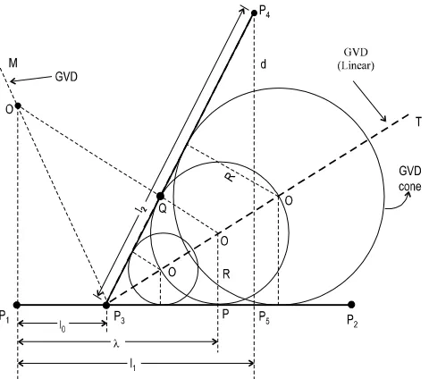
In this type of interaction between a pair of edges (interaction between an edge of one obstacle with an edge of another obstacle) as shown in the Fig. 2 [26]. How to construct the obstacle collision free path from S to the G when the obstacles are like this ? Consider two edges P1P2 and P3P4 of two obstacles O1 and O2 as shown in

the Fig. 2. Here, P3P4 is an edge interacting with P1P2 at

the point P3 [6], [25].

P₁P₂; P₃P_{4 - Two edges of obstacles O}1 and O2

meeting at the point P_{3 [1]} R - Radius of the GVD cone.

λ - Be the distance parameter measured along the edge P1P2 measured from P1.

l0 - Distance from P1 to P3 along P1P2.

l1 - Distance from P1 to P5 along P1P2.

l2 - Length of P3P4.

d - Perpendicular distance from P4 to P1P2.

The radius of the obstacle collision free path along P1P2

can be expressed by a piece-wise linear function of λ and is given by Eq. (1), where sgn denotes the signum function or the sign of the particular parameter l2 and d, l0

, l1 and l2 are as shown in the Fig. 3 [7], [24], [1].

R(λ) =

d

} 1 ) 1 (λ 1

{1 ) 1

(λ− _{0 0}− ₁+sgn − _{0 2}

. (1)

From this equation (1), we can come to a conclusion that [8] If ( λ− l

0 ) > 0 ; i.e., the point P is lying to the right of P3

; then, l

2 is positive , sgn ( ) is +.

If ( λ− l₀ ) < 0 ; i.e., the point P is lying to the left of P3 ;

Fig. 3 : Interaction between a pair of edges

First Method of Obtaining the obstacle

collision free path :

Consider a point P any where on the line P₁ P₂ and which is at a radial distance of λ from P1. Draw a ⊥

r

line (dotted) from P [9]. Find the length of this line ⊥r line (dotted) by using the Eq. (1) and mark the length (PO), where PO is the radius of the obstacle collision free path circle with O as the center. With O as center, draw a circle to pass through the points Q, P. Like this, go on taking different points (P’s) on the line P

1 P2 and which is

at a radial distance of different λ’s from P1. Go on

drawing ⊥r lines from P. Go on finding the length of these ⊥r _{lines (radii) using the formula, with their centers,}

go on drawing circles to touch the two edges. Go on joining all the centers of the obstacle collision free path circles. Thus, we get the obstacle collision free path from the source to the goal when the obstacles edges are straight lines [1].

Second Method of Obtaining the obstacle collision free path :

Bisect the angles P4 P3 P2 and P4 P3 P1 to get different point (O’s). With these points as centers, draw the circles with the radii as the perpendicular distances [11]. Join the centers of all the circles, we get the obstacle collision free path, which is nothing but the angle bisector P3 T [12]. Similarly, we get another angle bisector P3 M along which the robot or the object would move, the path being perpendicular to the previous path [10], [1].

L1

l₁

l2

d₂ d₁

F₁ P₁

P₃ P4

F2

P₂

GVD path linear

L₀

Fig. 4 : When the two edges P₁ P₂ and P₃ P₄ are parallel

Third Method of Obtaining the obstacle collision free path - Special Case of Interaction Between Two Edges :

When two edges P1 P2 and P3 P4 are parallel as shown in the Fig. 4, the obstacle collision free path is the mid-way path between the two edges of the obstacles [24]. Hence, to conclude, the interaction between a pair of edges is linear or a straight line [13]. If the robot or the object held by the tool / gripper moves along the obstacle collision free path, then definitely, there would be no collision of the object or the robot itself with the obstacles [14], [1].

Fourth Method of Obtaining the obstacle collision free path : Interaction Between a Vertex and an Edge

This is the second basic type of interaction while constructing a path between the vertex of an obstacle and an edge of another obstacle as shown in Fig. 6. Here, P1P2 is an edge and P3 is a vertex which is located at a perpendicular distance of d units from the edge P1P2 . The parameter λ represents the distance along the edge P1P2 measured from P1 .

The radius of the GVD is given by

R(λ) =

2d ) 1 (λ

d2 + − 1 2 _{or R(α) =}

( )

α

+

cos

1

d

. (2)

When λ = l1 or α = 0 ; R(α) = R(λ) = d 2 , i.e., midpoint of the perpendicular distance d .

−α α p1

GVD path (linear)

p2

O O O

R

R R

R p1

p2

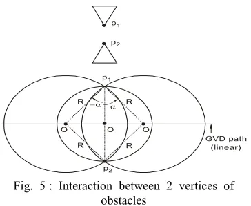
Fig. 5 : Interaction between 2 vertices of obstacles

Consider a point P at a distance of λ from P1 . Draw a

⊥r upwards from P . Find the radius of the GVD cone using the formula R(λ) . Measure this distance R along the ⊥r distance . Let it be PO = R(λ) . With O as center and PO as radius , draw a circle to pass through P . Like this, go on finding the centers of all the various circles . Join them . We get the GVD path . Therefore , the interaction between a vertex and a edge is a parabola .

Fifth Method of Obtaining the obstacle collision free path : Interaction Between a Pair of Vertices of 2 obstacles

This is the third basic type of interaction that has to be taken into consideration while constructing the GVD. P1 and P2 are two vertices of two obstacles which are separated by a distance of d units as shown in Fig. 5. Draw a line from P1 or P2 at an angle of α . Find the radius of the GVD cone using the radius formula R(α) =

d

2 cos α . Let it be P1O = P2O = R(α) . With R(α) as

radius and O as centre , draw a circle to pass through the points P1 and P2 . Like this , go on finding the center points of all the circles . Join the center points of all the circles , we get the shortest path. Hence, the interaction between a pair of vertices is a straight line . When α = 0 ,

it is d₂ , i.e., the mid point .

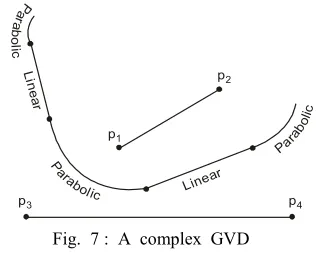
Sixth Method of Obtaining the obstacle collision free path - Complex path :

This is a path induced by a skew edge → combination of all the 3 basic types of interactions .

In a robotic work cell , there will be a number of obstacles . Hence , the path for the movement of the robot tool from the source to the goal comes across a number of edges and vertices of the different obstacles that comes along the path . Hence , the three types of interactions discussed above will not be sufficient to plan a obstacle collision free path in the 3D Euclidean space . A combination of the above three types of 3 paths is required. Such a diagram obtained is known as a complex path and is a combination of all the three types of the basic path’s .

as shown in the Fig. 7. Path between vertex P1 and edge P3P4 to the left and to the right of P1 is a parabola. Path between edge P1P2 and edge P3P4 to the left and to the right of P1P2 is a straight line. Path between vertex P2 and edge P3P4 to the left and to the right of P2 is a parabola .

Thus , a complex path is a combination of linear and parabolic paths . The path will consists of straight line segments and arcs and is also called as a complex graph .

4. MOTION HEURISTICS

Motion heuristics is the method of searching an obstacle collision free path in the free work space of the robot from the source to the destination by making use of search techniques such as the graph theory (AND / OR graphs), chain coding techniques and the state space search techniques (best first search, breadth first search) used in Artificial Intelligence [23]. The search techniques used in AI to find the path from the source S to the goal G are called as motion heuristics or the robot problem solving techniques [15]. The word ‘heuristic’ means to search , what to search ? an obstacle collision free path to search [16].

p3

p1

GVD path parabolic

O

O

O

O O

O O

− α α R

d

P

A1 p2

R

λ

p3

p2

p1

5.

P

S

&

S

R

We consider a workspace cluttered with obstacles, especially triangular obstacles. These triangular obstacles are placed either on the table or on the floor, which is simulated on the computer as a 2D rectangular workspace [22]. Using the mouse or using a rectangular coordinates, we specify the source coordinates ( x1 , y1 ) [17]. Similarly, using the mouse

or using rectangular coordinates, we specify the destination coordinates ( x2 , y2 ) [18].

A computer algorithm is written using the user-friendly language C++ to find the shortest path using the formula given in Eq. (1). The results of the simulation are shown in the Figs. 5 and 6 respectively [19]. The motion heuristics used in Artificial Intelligence is used to find the shortest path from the source to the goal [21]. Using this motion heuristics, a number of paths are available from the source to the goal, but it selects a shortest path which is the path shown in yellow color in the Fig. 6 [20], [1].

Fig. 8 : Instruction for entering the rectangular coordinates

Fig. 9 : Graph showing all the available free paths from S to G

6.

CONCLUSION

A method of finding an obstacle collision free path from the source to the goal when the workspace is cluttered with obstacles is developed using motion heuristics using an user friendly GUI developed in C++. This method is similar to the method of finding / searching a path by the humans.

The method was also implemented on a real time system, say a robot and was successful. Thus, the Artificial Intelligence which uses motion heuristics (search methods) is used to find the obstacle collision free path.

7. REFERENCES

[1]. Robert, J.S., Fundamentals of Robotics : Analysis and Control, PHI, New Delhi., 1992.

[2]. Klafter, Thomas and Negin, Robotic Engineering, PHI, New Delhi, 1990.

[3]. Fu, Gonzalez and Lee, Robotics : Control, Sensing, Vision and Intelligence, McGraw Hill, Singapore, 1995.

[4]. Ranky, P. G., C. Y. Ho, Robot Modeling, Control & Applications, IFS Publishers, Springer, UK., 1998.

[5]. T.C.Manjunath, Fundamentals of Robotics, Nandu Publishers, 5th Revised Edition, Mumbai., 2005.

[6]. T.C.Manjunath, Fast Track To Robotics, Nandu Publishers, 3nd _{Edition, Mumbai, 2005.}

[7]. Ranky, P. G., C. Y. Ho, Robot Modeling, Control & Applications, IFS Publishers, Springer, UK, 2005.

[8]. Groover, Weiss, Nagel and Odrey, Industrial Robotics, McGraw Hill, Singapore, 2000.

[9]. William Burns and Janet Evans, Practical Robotics - Systems, Interfacing, Applications, Reston Publishing Co., 2000.

[10]. Phillip Coiffette, Robotics Series, Volume I to VIII, Kogan Page, London, UK, 1995.

[11]. Luh, C.S.G., M.W. Walker, and R.P.C. Paul, On-line computational scheme for mechanical manipulators, Journal of Dynamic Systems, Measurement & Control, Vol. 102, pp. 69-76, 1998.

p3 p4

p₁

p₂

Para

bo

lic

L in_e

a r P a

ra

b

o

lic

P ar_ab

olic Linear

[12]. Mohsen Shahinpoor, A Robotic Engineering Text Book, Harper and Row Publishers, UK.

[13]. Janakiraman, Robotics and Image Processing, Tata McGraw Hill.

[14]. Richard A Paul, Robotic Manipulators, MIT press, Cambridge.

[15]. Fairhunt, Computer Vision for Robotic Systems, New Delhi.

[16]. Yoram Koren, Robotics for Engineers, McGraw Hill.

[17]. Bernard Hodges, Industrial Robotics, Jaico Publishing House, Mumbai, India.

[18]. Tsuneo Yoshikawa, Foundations of Robotics : Analysis and Control, PHI.

[19]. Dr. Jain and Dr. Aggarwal, Robotics : Principles & Practice, Khanna Publishers, Delhi.

[20]. Lorenzo and Siciliano, Modeling and Control of Robotic Manipulators, McGraw Hill.

[21]. Dr. Amitabha Bhattacharya, Mechanotronics of Robotics Systems, Calcutta, 1975.

[22]. S.R. Deb, Industrial Robotics, Tata McGraw Hill, New Delhi, India.

[23]. Edward Kafrissen and Mark Stephans, Industrial Robots and Robotics, Prentice Hall Inc., Virginia.

[24]. Rex Miller, Fundamentals of Industrial Robots and Robotics, PWS Kent Pub Co., Boston.

[25]. Doughlas R Malcom Jr., Robotics … An introduction, Breton Publishing Co., Boston.

[26]. Wesseley E Synder, Industrial Robots : Computer Interfacing and Control, Prentice Hall.

[27]. Carl D Crane and Joseph Duffy, Kinematic Analysis of Robot Manipulators, Cambridge Press, UK.

[28]. C Y Ho and Jen Sriwattamathamma, Robotic Kinematics … Symbolic Automatic and Numeric Synthesis, Alex Publishing Corp, New Jersey.

[29]. Francis N Nagy, Engineering Foundations of Robotics, Andreas Siegler, Prentice Hall.

[30]. William Burns and Janet Evans, Practical Robotics Systems, Interfacing, Applications, Reston Publishing Co.

[31]. Robert H Hoekstra, Robotics and Automated Systems.

[32]. Lee C S G, Robotics , Kinematics and Dynamics.

[33]. Gonzalez and Woods, Digital Image Processing, Addison Wesseley.

[34]. Anil K Jain, Digital Image Processing, PHI.

[35]. Joseph Engelberger, Robotics for Practice and for Engineers, PHI, USA.

on Robotics Research, Cambridge, MIT Press (1984), pp. 735-748.

[37]. Whitney DE., The Mathematics of Coordinated Control of Prosthetic Arms and Manipulators, Trans. ASM J. Dynamic Systems, Measurements and Control, Vol. 122 (1972), pp. 303-309.

[38]. Whitney DE., Resolved Motion Rate Control of Manipulators and Human Prostheses, IEEE Trans. Syst. Man, Cybernetics, Vol. MMS-10, No. 2 (1969), pp. 47-53.

[39]. Lovass Nagy V, R.J. Schilling, Control of Kinematically Redundant Robots Using {1}-inverses, IEEE Trans. Syst. Man, Cybernetics, Vol. SMC-17, No. 4 (1987), pp. 644-649.

[40]. Lovass Nagy V., R J Miller and D L Powers, An Introduction to the Application of the Simplest Matrix-Generalized Inverse in Systems Science, IEEE Trans. Circuits and Systems, Vol. CAS-25, No. 9 (1978), pp. 776.

Author Profile:

the significant contribution to the research (amongst all the researchers in all disciplines) in IIT Bombay. He was also instrumental in getting Research centres along with M.Tech programs in the colleges where he has worked so far. Apart from which, he had brought couple of grants for the conduction of various events like workshops & conferences where he worked. He visited Singapore, Russia, United States of America and Australia for the presentation of his research papers in various international conferences. His biography was published in 23rd edition of Marquis’s Who’s Who in the World in the 2006 issue. He has also guided more than 2 dozen projects (B.Tech. / M.Tech.) in various engineering colleges where he has worked so far apart from guiding a couple of research scholars who are doing Ph.D. in various universities.

Mrs. Ushaa Eswaran was born in Bangalore, Karnataka, India on Nov. 25, 1968 & received the B.E. Degree (Bachelor of Engg.) in Electronics & Instrumentation Engg. from the prestigious Annamalai University in the year 1989 with M.E. degree in Electronic Instrumentation Engg. in the year 2003 from the prestigious Andhra University, Vishakapatnam and pursuing her Ph.D. from the prestigious Jawaharlal Nehru Technological University (JNTU), Hyderabad in Electronics & Instrumentation Engg. She got a teaching experience of nearly 20 long years in various engineering colleges in Andhra Pradesh (Associate Professor-BVC engineering college, Assistant Professor-Gayathri Vidya Parishad Engineering College, Assistant Professor-Chaitanya Engineering College, Assistant Professor-Avanthi Engineering College) and is currently working as Vice-Principal, Professor & Head in the Electronics & Communication Engg. Dept in Siddharth Institute of Engg. & Technology, Puttur (Near Tirupathi), Andhra Pradesh, India for the past 6 years. She is also the chief placement officer in the SIET & looking after the placement activities. She has also worked in the industry in Micro chip computers – vasco d agama (Goa) as a customer support engineer / marketing executive & instructor for more than 2 years (Jan ’93 to Jan ’95). She also worked in the computer hardware industry as an hardware engineer in Pace