Hybrid Supervised Learning in MLP using Real coded GA and Back propagation

Hybrid Supervised Learning in MLP using Real-coded

GA and Back-Propagation

P. P. Sarangi

Dept. of CSE SEC, Mayurbhanj, India

B. S. P. Mishra

Dept. of CSE KIIT, Bhubaneswar, India

B. Majhi

S. Dehuri

ABSTRACT

This paper addresses a classification task of pattern recognition by combining effectiveness of evolutionary and gradient descent techniques. We are proposing a hybrid supervised learning approach using real-coded GA and back-propagation to optimize the connection weights of multilayer perceptron. The following learning algorithm overcomes the problems and drawbacks of individual technique by introducing global and local adaptation strategies. The behavior of the proposed algorithm is observed by the experimental results on a couple of popular benchmark datasets. The results of our algorithm are compared with training algorithms based on conventional back-propagation and real-coded genetic algorithm. Finally we realize that proposed hybrid learning algorithm outperforms back-propagation and real-coded genetic algorithm based training the multilayer perceptron.

Keywords:

Gradient descent; Generalization

1. INTRODUCTION

Classification is one of the most recurrently encountered decision making tasks of pattern recognition. A classification problem occurs when an object needs to be assigned into a predefined class (group) in decision space based on a number of features (attributes) from feature space [3].Nowadays, neural networks have recognized by research community as an important tool for classification with immense studies concerning training. Most widely used neural network model for classification is multilayer perceptron (MLP) based on one or more sequentially connected layers of perceptrons. Multilayer perceptron model considered in this paper belongs to the feedforward neural networks. In classification first, the network is trained on a set of paired data to evolve a set of connection weights and second, then the network is ready to test a new set of data [4]. The most popular and widely used training algorithm to estimate the values of the weights is the back-propagation (BP) algorithm [11], follows the principle of gradient descent technique. Because of back-propagation algorithm, multilayer perceptrons are widely employed in many real problems and can approximate any non-linear complex functions with arbitrary accuracy. Despite of its popularity, back-propagation algorithm has drawback of slow error convergence rate and being trapped at local minima. Another technique, global search based optimization algorithms are being used as learning method for feedforward neural networks. Many researchers have introduced evolutionary algorithms to optimize the neural networks weights globally in order to avoid the local minima that so often appear in complex problems. Davis [5] showed how any neural network can be rewritten as a type of genetic algorithm

called a classifier system and vice versa. Whitley [6] attempted successfully to train feedforward neural networks using genetic algorithms. Sexton, Dersey, and Jhonson [7]. Gupta and Sexton [8] compared back-propagation with a genetic algorithm for neural networks training. X. Yao [9] gave new dimension to neural networks. Sankar K. Pal and Dinabandhu Bhandari [10] used binary-coded GA for selection of optimal weights in MLP. Whitley, Darrell, Starkweather, Timothy, and Christopher Bogart [16] hybridized genetic algorithms and neural networks for optimizing connections and connectivity. J. D. Schaffer, Whitley and L. J. Eshelman [19] wrote a survey on combinations of genetic algorithms and neural networks. H. Hasan Örkcü, HasanBal [2] used binary and real coded genetic algorithms for optimization of the connection weights of more than one hidden layers in the MLP. In this paper we have represented all connection weights as real numbers in the genetic algorithms. Genetic algorithms (GAs) based learning is used to find near-optimal solutions globally from search space without computing gradient information. Original genetic algorithms use binary string vector representation similar to the chromosome structure of biology. But binary GA has some disadvantages based learning main objective is to improve accuracy of the network and no consideration is given to the speed of convergence and local error. Here, our focus is to first apply GA leaning and next the gradient descent algorithm in multi-layer perceptron to optimize the best connection weights and minimize local errors with fast convergence. We have found that our approach not only succeeds in its task but it outperforms back-propagation, the standard training algorithm.

The paper is structured as follows: Sections 2 deals an overview of neural networks and genetic algorithms respectively with a special emphasis on their strengths and weaknesses; Section 3 focuses on the detail of proposed algorithm; Section 4 describes empirical evolution of proposed algorithm on 11 real world data sets with their result analysis; Section 5 provides conclusions about our work and suggestions for future work.

2. BACKGROUND STUDY

2.1. Multi-layer perceptron training with

back-propagation

referred to in literature as neurocomputers, connectionist networks, parallel distributed processors, etc [12]. Neural networks consist of number of simple processing units called neurons and unidirectional communicational channels called connections (links).

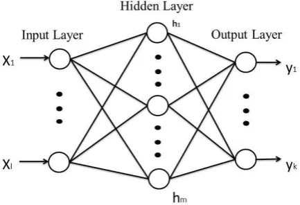
Fig 1: Schematic representation of multilayer perceptron

The figure 1 shows the architecture of feed forward neural network, most common form of it is multi-layer perceptron. The units are organized in several layers, namely an input layer, one or more hidden layers, and an output layer. We have used in our experiment, a three layer feedforward neural network with m inputs, k outputs and l hidden neurons. Each neuron of both hidden and output layer uses hyperbolic tangent function f (x) =

as activation function. The

output of thehidden node h (1 ≤h ≤l) and output node q (1 ≤q ≤k) can be expressed as:

, (1)

, (2) respectively, where W = the connection weight vector connects input nodes to hidden node h, V = the connection weight vector connects hidden nodes to output node k, X = the input vector for each hidden node and Z = the input vector foreach output node. and are the responses of hidden and output neuron of node h and node q, respectively. bh and bq are the biases for

hidden node h and output node q respectively. Most commonly used connection weights training algorithm for multi-layer perceptron is back-propagation. The idea of connection weights training in multi-layer perceptron is usually formulated as minimization of an error function, such as mean square error (MSE) between target (d)and actual (o)outputs averaged over all training examples. For a given training set, back-propagation learning may proceed in one of the two basic ways: sequential (on-line or pattern) mode and batch mode. In this paper we used batch learning in the experiment to adjust connection weights after the presentation of all the training examples that constitute an epoch. Thus net mean square error (MSE) function for a given neural network weight vector w is described as E(w);a value which is total sum of error of each neurons of the output layer of all training samples.

(3)

One method for minimization of error by repeatedly updating the weights of the net in the back propagation algorithm is to apply the principle of gradient descent as:

(n) (4)

where a positive number is called learning-rate parameter of the back-propagation algorithm, the local gradient of a layerj, and n is the number of the iteration in the training. The equation (4) is also called delta rule. The learning-rate controls the descent.A large value enables back-propagation to move faster to the target weights by reducing error of the neural network but it may not reach at minimum error of the error curve every time and rather oscillate. To avoid oscillation because of increasing the rate of learning, it is to modify the delta rule the equation (4) by including a momentum term. The following equation is called the generalized delta rule:

(n)+ (5)

Again a term hdec is subtracted from equation (5), hdec is the decay factor 0.01 > hdec> 0 enables only those weights that help to minimize the error to survive and hence improve the generalization capability of the network.

In addition, another improvement in learning algorithm is stopping rule to control when training ends. It is necessary due to the overfitting (overtraining) phenomenon.

2.2. Real-coded genetic algorithm

Genetic algorithms are randomized search algorithm based on the principle of natural selection and natural genetics. The characteristic of genetic algorithms are population-based evolution, survival of the fittest, directed stochastic, derivative-free. GAs performs the search process in four stages: initialization, selection, crossover, and mutation [13].GAs has been successfully incorporated in a wide rage of applications. GAs are robust, the reasons for this are [14] : 1) GA can solve hard problems quickly and reliably, 2) GAs are easy to interface to existing simulations and models, 3) GAs are extensible and 4) GAs are easy to hybridize. The binary coding representation of chromosomes encounter certain difficulties when dealing with continuous search spaces with large dimensions and a great numerical precision is required [15]. These difficulties are: more computing time for coding and decoding of chromosomes, premature convergence, and hamming cliff problem. Since the performance of binary-coded genetic algorithm for continuous optimization problems are not effective for continuous search space that led towards the use of real-coded genetic algorithm. In real-coded GA the representation of chromosomes are candidate solutions is very close to variables of the problem that means there are no difference between the genotype and the phenotype. The size of chromosome is number of genes that equals to number of variables the objective function have in a problem. In this paper size of chromosome is the total weights of the neural network and the value of genes are same as the value of weights.

2.2.1 Outlines of simple genetic algorithms

iterations called generations, chromosomes advances toward better solutions by selection of high fitness values in the population and through crossover and mutation. The structure of GAs as follows.

Simple_Genetic_ Algorithm ()

{

initialize population;

evaluate population;

while (termination_criteria_not_satisfied)

{

select parents for mating pool;

perform crossover;

perform mutation;

new generation after crossover and

mutation;

Evaluate population;

}

}

Fig 2: Structure of simple genetic algorithms

3. PROPOSED HYBRID SUPERVISED

TRAINING ALGORITHM

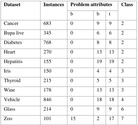
Traditional back-propagation algorithm adapts gradient information of error function to optimize the connection weights of the neural network but several times it may get stuck to local optimum easily. GAs has good exploration and exploitation characteristics that lead towards near optimal solution in a complex non-linear search space. Hence GA has been extensively used in neural networks weights optimization and is known as successful alternative approach to back-propagation algorithm. Several studies have been used GAs as training algorithm in multilayer perceptron and its performance compared with back-propagation that the former outperforming the latter in most applications. Moreover it is difficult to use binary-coded genetic algorithms for continuous search space with large dimensions and a great numerical precision. To overcome these problems it seems more natural to represent the genes of a chromosome directly as real numbers for applications with variables in continuous domain. Genetic algorithms based on real number representation of chromosomes are called real-coded genetic algorithms. In RGA the size of a chromosome is same as length of the vector which is the solution of the problem but in BGA it is not so [1]. However in RGA proper selection of genetic operators are very important for specific applications. In the present classification problem, the neural networks training using RGA suffers from premature error convergence that is earlier in training using BGA. In this paper an attempt has been taken to propose a hybrid supervised learning algorithm by integrating both real-coded genetic algorithms and back-propagation methods together to alleviate the premature error convergence problem of RGA and to get stuck in local minimum of MLP in the training of multilayer perceptron. In the simulation of the proposed algorithm, it has been observed that hybrid training algorithm outperforms the individual training methods of multilayer perceptron. Figure 2

shows the framework of hybrid real-coded genetic algorithm and back-propation algorithm

.

Fig 3: Framework of hybrid algorithm for classification

3.1Encoding connection weights and initial

population

In [1] proposed, number of connection weights in the network are the parameters of a chromosome. For L number of layers, number of parameters is

P = .

Each parameter is represented a real value in a range of (-1, 1). In addition to that more number of chromosomes in the population results in lesser number of generations to be executed for convergence but takes higher processing time for each generation.

3.2 Determine fitness function

Here, the network with more error, the fitness value is less and vice versa, decreasing overall error function F (E) may be represented as increasing function

F (E) =

Where is the total mean square error of individual

chromosome and a MSE normalization operation applied on that chromosome total MSE, which is its fitness value.

3.3 Fitness scaling or fitness shifting

3.4 Genetic operators

Genetic operators are the basic search mechanisms of the GA for creating new points based on the existing population. Selection operator performs exploitation of promising candidates in every generation. Reproduction of new points (children) from the selected points (parents) using the two genetic operations: crossover and mutation that leads to exploration of new parts of the search space. Crossover produces two new individuals (children) from two existing individuals (parents), whereas mutation alters one individual to produce a single individual. In this work, arithmetic crossover and non-uniform-mutation function have been used [17] in real-coded genetic algorithms.

3.4.1 Crossover operator

Let us assume that and are two chromosomes selected for the application of crossover operator. For the arithmetic crossover operator then two offspring, = ( , k = 1, 2, are generated, where and . λ is a positive constant and in the experiments, λ is set to 0.28.

3.4.2 Mutation operator

Let us assume the nonuniform mutation operator is applied in a generation r, and is the maximum number of generations, new offspring can obtain as

∆(r, y) = y (1 -

where is a random number either 0 or 1, b is a parameter that determines the degree of dependence on the number of iterations, in our experiments, b is set to 0.5. The random value rand lies in a range [0, 1].

3.5 Proposed algorithm for MLP

STEP 1. initialize the RGA parameters

STEP 2. initialize the population with real values in the domain for each neuron’s connection weights and bias to its correspondent gene segments

STEP 3. while new gen. is less than equal to MaxGen. Do {

STEP 4. the fitness of a chromosome is determined by MSE

STEP 5. sort minimum fitness values

STEP 6. if first fitness value is less than equal to min. error then select best solution for MLP then goto step 9

STEP 7. select parents for reproduction based on their fitness

STEP 8. new population by crossover and mutation

STEP 9. goto step 1 for new generation}

STEP 10. initialize parameters of back-propagation learning

STEP 11. initialize weights of the MLP using best solution of RGA

STEP 12. while new epoch is less than equal to MaxEpoch or error converges to Min Error do

STEP 13. update weights to minimize error using back-propagation with training data

STEP 14. end while

STEP 15. evaluate performance of classification with test data

STEP 16. end while

4. EXPERIMENTAL STUDY

4.1 Experimental real world datasets

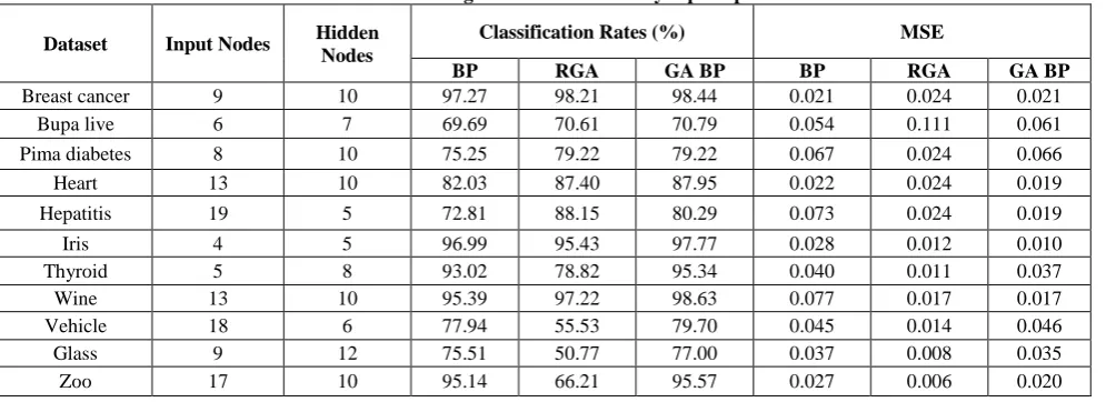
In this section numbers of experiments were conducted with standard datasets. Eleven classification problems were verified in the experiment. In Table 1 lists a summary of the used datasets along with following attributes: problems and the number of instances, the number of binary (b), continuous (c) features in the dataset, number of classes. The classification problems were obtained from the UCI repository [20]. In pattern classification, the total set of patterns in the dataset divided into three different set of partitions forming training, validation and test sets prechelt [17]. A popular and very useful form to use validation set in neural network is early stopping. In this paper the validation set was used for testing the performance of the network in the training phase, it is necessary to avoid the overtraining phenomenon. Here initially the datasets were divided into two segments like sixty and forty percent of data, former was used for training and later for testing sets. Again the training segment divided into two parts like twenty and forty percent of data. The later segment was

used for training and former segment for validation sets. Before partition of the dataset, we were normalized the dataset using z-score or max-min normalization techniques.

The proposed algorithm is compared with back-propagation and real-coded GA based training multilayer perceptron. BP, Real-coded GA based training and proposed one was implemented and analyzed using matlab.

Table 1: Summary of used classification problems

Dataset Instances Problem attributes Class

b b t

Cancer 683 0 9 9 2

Bupa live 345 0 6 6 2

Diabetes 768 0 8 8 2

Heart 270 0 13 13 2

Hepatitis 155 0 19 19 2

Iris 150 0 4 4 3

Thyroid 215 0 5 5 3

Wine 178 0 13 13 3

Vehicle 846 0 18 18 4

Glass 214 0 9 9 6

4.2 EXPERIMENTAL PREPARATION

2. The real-coded genetic algorithms used real encoding to represent chromosomes

3. Each chromosome in the population represents the neural network architecture

4. The length of the chromosome is the total number of connection of the network

5. Synaptic weights of the neural network are represented by real values in a domain [-1, 1]

6. Population size: 10

7. Linear fitness scaling were used to compress the range of fitness to two

8. Roulette wheel selection or Rank based roulette selection were used in the mating pool

9. Crossover rate: 0.9

10. Arithmetic crossover operator was used 11. Mutation rate: 0.7

12. Non-uniform mutation operator was used

13. Elitism the best chromosomes are preserved for the next generation was used

14. Number of generation for each experiment: 50 to 100 15. The multilayer perceptron had only one hidden layer, number of neurons in this layer was optimized by trial and error method as mentioned in table 2.

16. The transfer function of the hidden layer and output layer are bipolar sigmoid functions

17. The learning rate and momentum parameter of the BP is 0.01 and 0.9

18. Each classifier repeatedly executed ten times for one over all datasets and average accuracy mentioned in Table 2

4.3 EXPERIMENTAL RESULT

ANALYSIS

Each training algorithm runs ten times over all datasets mentioned in Table 1and the average accuracy of the classifier (the percentage of samples that it correctly classified) is computed. The results were obtained for each training technique by the optimization of the connection weights of the multilayer perceptron. The fitness function values (errors)

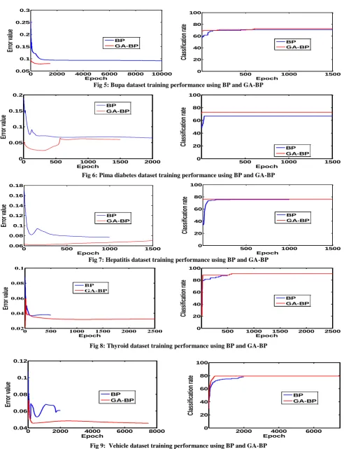
were normalized and obtained average over total number of training samples. Finally in batch learning mean square error (mse) was obtained that updated the connection weights of the MLP. Moreover the classification rate of the test set obtained in the training of the MLP using different training algorithms, presented in Table 2. Figure 1 to Figure 11 show the graphs comparing the mean square error (mse) and classification rates of the investigated training algorithms over all datasets. The proposed algorithm obtained the best results in the most dataset where RGA based training fails. By taking advantage of global optimization, early stopping, and weight decay proposed algorithm takes less computational time than RGA based training algorithm. Similarly, the problem of local minimum of BP algorithm observed many times in running the training algorithm number of times over all datasets. It leads worst performance in the experiments that could be avoided by proposed algorithm.

From the experiments, it has revealed that by a large crossover rate and a higher mutation rate the proposed algorithm needs small number of generations. Here we used 50 to 100 number of generation with 0.9 crossover and 0.07 mutation rates to train the MLP at initial stage. Then BP algorithm takes small number of epochs to optimize the connection weights of MLP with less mean square error. In RGA based training, maximum generation number was chosen 10000.

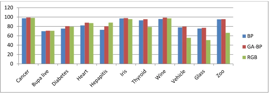
It is analyzed from Table 2 that for almost all datasets the classification rate of the proposed training algorithm outperforms classical back-propagation and real-coded GA. But datasets like thyroid, vehicle, glass and zoo the RGA based training obtained poor classification rates even worse than back-propagation algorithm. Thus it is clearly observed from the table that where RGA based training not performed well there proposed training algorithm obtained best results. Moreover in hepatitis dataset RGA based training produced best result than proposed training algorithm. Figure 4 shows the graphs comparing the performances of the investigated training algorithms of multilayer perceptron. The proposed training algorithm obtained best results regarding classification accuracy in percentage except hepatitis dataset. From the results we realized that in the proposed algorithm, initially RGA evolved a better search space globally in few generations then BP locally optimized the connection weights of the neural network.

Table 2: Training results of the multilayer perceptron

Dataset Input Nodes Hidden Nodes

Classification Rates (%) MSE

BP RGA GA BP BP RGA GA BP

Breast cancer 9 10 97.27 98.21 98.44 0.021 0.024 0.021

Bupa live 6 7 69.69 70.61 70.79 0.054 0.111 0.061

Pima diabetes 8 10 75.25 79.22 79.22 0.067 0.024 0.066

Heart 13 10 82.03 87.40 87.95 0.022 0.024 0.019

Hepatitis 19 5 72.81 88.15 80.29 0.073 0.024 0.019

Iris 4 5 96.99 95.43 97.77 0.028 0.012 0.010

Thyroid 5 8 93.02 78.82 95.34 0.040 0.011 0.037

Wine 13 10 95.39 97.22 98.63 0.077 0.017 0.017

Vehicle 18 6 77.94 55.53 79.70 0.045 0.014 0.046

Glass 9 12 75.51 50.77 77.00 0.037 0.008 0.035

Fig 5: Bupa dataset training performance using BP and GA-BP

Fig 6: Pima diabetes dataset training performance using BP and GA-BP

Fig 7: Hepatitis dataset training performance using BP and GA-BP

Fig 8: Thyroid dataset training performance using BP and GA-BP

Fig 9: Vehicle dataset training performance using BP and GA-BP

0 2000 4000 6000 8000 10000

0.05 0.1 0.15 0.2 0.25 0.3 Epoch

Er

ro

r v

al

ue

500 1000 1500

0 20 40 60 80 100 Epoch

Cl

as

si

fic

ati

on

ra

te

0 500 1000 1500

0.06 0.08 0.1 0.12 0.14 0.16 0.18 Epoch

Er

ro

r v

al

ue

500 1000 1500

0 20 40 60 80 100 Epoch

Cl

as

si

fic

ati

on

ra

te

0 500 1000 1500 2000

0 0.05 0.1 0.15 0.2 Epoch

Er

ro

r v

al

ue

500 1000 1500

0 20 40 60 80 100 Epoch

Cl

as

si

fic

ati

on

ra

te

0 500 1000 1500 2000 2500

0.02 0.04 0.06 0.08 0.1 Epoch

Er

ro

r v

al

ue

500 1000 1500 2000 2500

0 20 40 60 80 100 Epoch

Cl

as

si

fic

ati

on

ra

te

2000 4000 6000

0 20 40 60 80 100 Epoch

C

la

ss

ifi

ca

tio

n

ra

te

0 2000 4000 6000 8000

Fig 10: Performances of the investigated training algorithms of MLP

5. CONCLUSION

Feed forward neural networks training using back-propagation, real-coded GA, and proposed hybridization of a real-coded GA and back-propagation algorithms have been discussed in this paper. In the experiment, proposed hybrid training algorithm has been compared with back-propagation and real-coded GA using several real world standard datasets. From experimental results it is cleared that real-coded GA based training algorithm not provides the highest accuracy and generalization results for all datasets. Although RGA produce global optimal solutions, it has shown RGA suffers from premature error convergence in complex problems that can lead to the training failure. Similarly, the back-propagation algorithm has better local searching ability but its performance depends on the input sequence to reach at global optimum solution. Because of that back-propagation algorithm not always performs better and traps in local minima. Again when problems are more complex, back-propagation most often fails because of its inherent gradient decent technique. In case of complex problems, large connection weight parameters of the neural networks increase the size of chromosome. The longer the size of chromosome needs more generations to globally optimize the weights parameters. Hence genetic algorithms are slower in the cost of better performance than where back-propagation fails. To alleviate the problems of premature convergence and more training time of genetic algorithms and getting stuck in local minimum of back-propagation the hybrid algorithms has been adopted in this paper. The simulation of hybrid algorithm starts training with real-coded GA for several generations then uses that global information of RGA solution as initial weights of the neural network to commence the back-propagation algorithm for local convergence of error. The experimental results of the proposed hybrid algorithm improves the training error convergence rate where real-coded GA and back-propagation fail, that leads to better accuracy and generalization. It also revealed that the proposed algorithm outperforms back-propagation and real-coded GA training algorithm without trapping in local minimum. Moreover proposed algorithm takes less training time than real-coded GA based training algorithm. In future this work

will be extended in solving real world problems in image processing, bioinformatics, robotics and business.

6. REFERENCES

[1] P.P.Sarangi, B.Majhi and M.Panda, "Performance Analysis of Neural Networks Training using Real Coded Genetic Algorithm", International Journal of Computer Applications 51(18):30-36, 2012.

[2] H. HasanÖrkcü, HasanBal, "Comparing performances of back-propagation and genetic algorithms in the data classification", Expert Systems with Applications, Volume 38, Issue 4,Pages 3703-3709,2011.

[3] Zhang, G., “Neural networks for classification: a survey”, IEEE Transactions on Systems, Man, and Cybernetics, Part C 30(4): 451-462, 2000.

[4] S. B. Kotsiantis, “Supervised Machine Learning: A Review of Classification Techniques”, Informatica31

249-268, 2007

[5] L. Davis, “Mapping Classifier Systems into Neural Networks'', Conference on Neural Information Processing Systems, Morgan Kaufimann, 1988.

[6] Whitley, Darrell, "Applying Genetic Algorithms to Neural Network Problems," International Neural Network Society p. 230, 1988.

[7] Randall S. Sexton, Robert E. Dorsey, John D. Johnson, “Optimization of Neural Networks: A Comparative Analysis of the Genetic Algorithm and Simulated Annealing”, European Journal of Operational Research, volume 114, issue 3,page 589-601, 1999.

[8] Gupta, J. N. D., & Sexton, R. S. Comparing back-propagation with a genetic algorithm for neural network training. Omega, 27, 679–684.

[9] X. Yao, Evolving artificial neural networks, Proc. IEEE 87 (9), 1423–1447, 1999.

[10] Pal S. K. and BhandariD.”Selection Of optimal set of weights in a layered network using genetic algorithm”, Information Sciences, Vol: 80, Pages: 213-234,1994. [11] D.E. Rumelhart, G.E. Hinton, R.J. Williams, Learning

representations by back-propagating errors, Nature 323 533-536, 1986

0 20 40 60 80 100 120

BP

GA-BP

[12] Simon Haykin, “Neural Networks: A comprehensive foundation,” Pearson Education Asia, Seventh Indian Reprint, 2004.

[13] J.H. Holland, Adaptation in Natural and Artificial Systems, the University of Michigan Press, 1975. [14] D.E. Goldberg, Genetic Algorithms in Search,

Optimization, and Machine Learning, Addison-Wesley, New York, 1989.

[15] F. Herrera, M. Lozano, J.L. Verdegay, Tackling Real-coded Genetic Algorithms: Operators and Tools for Behavioral Analysis, Artificial Intelligence Review 12: 265-319, Kluwer Academic Publishers 1998.

[16] Whitley, Darrell, Starkweather, Timothy, and Christopher Bogart, “Genetic Algorithms and Neural Networks: Optimizing Connections and Connectivity,” ParallelComputing, 14, pp. 347-361,1990.

[17] Deep, K., & Thakur, M. A new crossover operator for real coded genetic algorithms. Applied Mathematics and Computation, 188, 895–911, 2007.

[18] Prechelt, L.: Proben1, “A Set of Neural Network Benchmark Problems and Benchmarking Rules”. Technical Report 21, FakultÄat fÄur Informatik UniversitÄat Karlsruhe, 76128 Karlsruhe, Germany, 1994.

[19] Schaffer J. D., D. Whitley, and L. J. Eshelman, “Combinations of Genetic Algorithms and Neural Networks: A Survey of the State of the Art,” Proceedings of the IEEE Workshop on Combinations of Genetic Algorithms and Neural Network.

[20] UCI repository of machine learning databases, Department of Information and Computer Sciences,

University of California, Irvine,