A Clustering Algorithm for Discovering Varied Density Clusters

(1)

A Clustering Algorithm for Discovering Varied Density Clusters

Ahmed M. Fahim

Department of computer science, Faculty of Science, Suez University, Suez, Egypt

,

Checked at Department of computer science, Faculty of Science and Human Studies, Prince Sattam bin Abdul Aziz

University, Aflaj, KSA.

---*---Abstract -**

Spatial data clustering is one of the

important data mining techniques for extracting knowledge from large amount of spatial data collected in various applications, such as remote sensing, GIS, computer cartography, environmental assessment and planning, etc. many useful spatial data clustering algorithms have been proposed. DBSCAN is the most popular density clustering algorithm, which does not limit itself to shapes of clusters and handles the noise effectively. However, DBSCAN has a trouble in finding out all clusters from datasets with varied densities, because it depends on a globular value for its parameter Eps. This paper presents enhanced DBSCAN which clusters spatial databases that contain clusters of varying densities effectively. The idea is to allow varied values for the Eps parameter according to the local density of the starting point in each cluster. The clustering process starts from the highest local density point towards the lowest local density one. And the value of Eps varies according to the local density of the initial point in current cluster. For each value of Eps, DBSCAN is adopted to make sure that all density reachable points with respect to current Eps are clustered. At the next process, the clustered points are ignored, to avoid merging among denser clusters with sparser ones. Varied synthetic datasets in 2-dimension are used to evaluate the efficiency of the proposed enhanced DBSCAN algorithm.

Key Words:

DBSCAN, Data Clustering, Density

Clustering.

1. INTRODUCTION

Spatial data clustering is one of the promising techniques of data mining, which groups a set of objects into classes or clusters so that objects within a cluster have high

similarity in comparison to one another, but are dissimilar to objects in the other clusters. Based on a general definition, data clustering algorithms can be classified into four categories; (1) partitioning, (2) hierarchical, (3) density-based and (4) grid-based methods. However, some algorithms may fall into more than one category. By clustering one can identify dense and sparse regions and, therefore, discover overall distribution patterns. Finding clusters in data is challenging when the clusters are of widely differing sizes, shapes and densities and when the data contains noise and outliers. Although many algorithms exist for finding clusters with different sizes and shapes, there are a few algorithms that can detect clusters with different densities.

Basic density based clustering techniques such as DBSCAN [4] and DENCLUE [5] treat clusters as regions of high densities separated by regions of no or low densities. So they are able to suitably handle clusters of different sizes and shapes besides effectively separating noise and outliers. But they may fail to identify clusters with varying densities unless the clusters are well separated by sparse regions.

There are some algorithms which handle clusters of different densities, like OPTICS [1] but it does not produce explicit clusters. Traditional DBSCAN may have trouble

(a) (b)

(c)

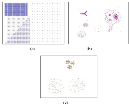
Fig -1: Clusters with varying densities

[image:1.595.318.544.510.692.2]

(2)

dataset shown in Fig. 1.a, DBSCAN fails to find the four clusters, because this data set contains four levels of density, the clusters are not totally separated by sparse

regions and the value of Eps is globular for the dataset. So

we need an approach able to stop clustering expanding at different levels of density. In Fig. 1.b there are two problems; they are in the smallest sparse cluster and the largest cluster that contains three dense clusters within it. In Fig. 1.c, DBSCAN discovers only the three small clusters and considers the other two large clusters as outliers or merge the three small clusters in one cluster to be able to find the other two large clusters. This problem can be

solved by using different Eps for each local density in

dataset.

This paper introduces an enhanced version of the DBSCAN algorithm which is able to discover clusters with varying densities. It selects a suitable value for its parameter Eps for each cluster, based up on the local density of the starting point in each cluster, and adopts the

traditional DBSCAN for each value of Eps. The idea of the

proposed algorithm depends on discovering the highest

density clusters at first, and then the Eps is adapted to

discover next low density clusters with ignoring the previously clustered points. The proposed algorithm

requires two input parameters; they are Minpts and

Maxpts. The Maxpts allows the value of Eps to be varied in each cluster according to the local density of the initial

point in the current cluster. The Minpts determines the

lowest level of density allowed within the cluster, while the Maxpts limits the highest level of density allowed within the cluster in addition to it controls the values of

Eps neighboring radius of the traditional DBSCAN

algorithm. We can note that the DBSCAN starts to create a cluster from any core point, while the enhanced DBSCAN starts cluster creation process from the highest density core point. We refer to this core point as starting point or initial point.

This paper is organized as follows. Section 2 surveys the main definitions of DBSCAN. Section 3 briefly surveys some of density clustering methods. The proposed algorithm is presented in section 4. Section 5 presents some experimental results to evaluate the algorithm, and section 6 presents a conclusion.

2

.

DENSITY BASED CLUSTERING (DBSCAN)

Since the proposed algorithm is an enhanced version of DBSCAN algorithm, it is important to review the main definition of DBSCAN algorithm, for details see [4].

Let D is a database of N points in d-dimensional space Rd_.

The distance between two data points p and q is given by

the Euclidean distance and denoted by d(p,q). The

DBSCAN depends on the following definitions:

 The Eps-neighborhood of a point p, denoted by

NEps(p), is defined by NEps(p) = {qD | d(p,q) ≤ Eps}.

 A point p is directly density-reachable from a point q

wrt. Eps and Minpts if pNEps(q) and |NEps(q)| ≥

Minpts (core point condition).

 A point p is density-reachable from a point q wrt. Eps

and Minpts if there is a chain of points p1, ..., pn, p1 = q,

pn = p such that pi+1 is directly density-reachable from

pi.

 A point p is density-connected to a point q wrt. Eps

and Minpts if there is a point o such that both, p and q

are density-reachable from o wrt. Eps and Minpts.

 A cluster C wrt. Eps and Minpts is a non-empty subset

of D satisfying the following conditions:

 p, q: if pC and q is density-reachable from p

wrt. Eps and Minpts, then qC. (Maximality)

 p, qC: p is density-connected to q wrt. Eps and

Minpts. (Connectivity)

 If C1,..., Ck be the clusters of the database D wrt.

parameters Epsi and Minptsi, i = 1, ..., k. Then the noise

is defined as the set of points in the database D not

belonging to any cluster Ci, i.e. noise = {pD |  i:

pCi}.

 If d(p,q) ≤ Eps , q is core point and |NEps(p)| Minpts

then p is a borderpoint.

DBSCAN searches for clusters by checking the Eps

neighborhood of each point in the database. If the Eps

neighborhood of a point P contains Minpts or more, a new

cluster with P as core point is created. Then DBSCAN

iteratively collects directly density-reachable points from these core points, which may involve the merge of a few density-reachable clusters. The process terminates when no new points can be added to any cluster. In DBSCAN the

Minpts is fixed to 4 points, and the number of clusters

discovered depends on the Eps value which is fixed during

the execution process, and this value is not suitable for discovering clusters with different densities except when the clusters are totally separated. But when the clusters are not totally separated the DBSCAN algorithm faces the problem of varying densities and produces inaccurate clusters.

3. RELATED WORKS

The DBSCAN (Density Based Spatial Clustering of Applications with Noise) [4] is a basic density based

clustering algorithm. The density associated with a point p

is obtained by counting the number of points in a region of

specified radius Eps around p. A point with density greater

than or equal to a specified threshold Minpts is treated as

(3)

that are maximal with respect to density-reachability. DBSCAN can find clusters having varying sizes and shapes, but there may be wide variation in local densities within a

cluster since it uses global density parameters Minpts and

Eps, which specifies only the lowest possible density of

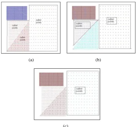
any cluster without restricts the highest possible density. Fig. 2 shows the results from applying the DBSCAN on the dataset in Fig. 1.a.

From Fig. 2, we note that for some datasets we need many

different values for the Eps parameter of DBSCAN

algorithm to discover clusters with different densities, and we cannot depend on a single value for this sensitive parameter. This problem motivates us to propose an enhanced version of DBSCAN which is able to discover clusters from datasets having varying densities.

To find clusters that are naturally present in a dataset, very different local densities needed to be identified and separated into clusters. There are some improvement have been done on the DBSCAN algorithm. But these improvements focus on the scalability of the algorithm by reducing the number of query region [3]. This has been

done by sampling the points in the Eps neighborhood of

core point p and marking these points as Marked

Boundary Objects (MBO), for each of these MBOs, the closest point in the Eps-neighborhood -as in Fig. 3- is identified and selected as a seed. If the same point is

identified as the nearest point for more than one MBO then this point must be regarded only once as a seed. Therefore total number of seeds selected may be less than or equal to eight in 2-dimensional case. In general, if the

points are of dimension d, then there will be (3d_{-1) MBOs,}

2d_{quadrants and number of seeds selected is at most 3}d_-1.

This number is lower than the corresponding number in DBSCAN. IDBSCAN [3] yields the same quality of DBSCAN

but is more efficient.

Another algorithm is introduced to improve the efficiency of DBSCAN by merging between the k-means and IDBSCAN, this algorithm is known as KIDBSCAN [9]. K-means yield the core points of clusters. Then, clusters are expanded from these core points by executing IDBSCAN.

The purpose of the k-means is to determine the k highest

density center points and the points that are closest to the center points. These points are moved to the front of the data. And the IDBSCAN start the expansion of clusters from high density center points, this process reduces the number of redundant steps and increases efficiency. In [8] the authors introduced VDBSCAN. Firstly, VDBSCAN calculates and stores dist for each point and partition k-dist plot. K-k-dist plot is drawn for selection of parameters

Epsi and analysis of density levels of the dataset. Secondly,

the number of densities is given intuitively by k-dist plot.

Thirdly, choose parameters Epsi for each density. Fourthly,

scan the dataset and cluster different densities using

corresponding Epsi. And finally, display the valid clusters

corresponding with varied densities. VDBSCAN has two

steps: choosing parameters Epsi and cluster in varied

densities. This method depends on seeing several smooth curves connected by greatly variational ones, and in many cases we see only one smooth curve, referring to our experimental results we see only one curve in dataset 8 and two curves in dataset 7 and more than 12 curves in 4-dist plot in dataset 3. And this is only true for dataset 4 where the points of each region are uniformly distributed. DDSC (Density Differentiated Spatial Clustering) [2] is proposed. It is an extension of the DBSCAN algorithm to detect clusters with differing densities. Adjacent regions

(a) (b)

(c)

Fig -2: (a) DBSCAN discovers only the most density

cluster (Eps=0.25). In (b) it discovers two clusters

satisfying the lowest possible density (Eps=0.4). In

(c) it merges the two clusters in (b) with the intermediate points to produce only one cluster

(Eps=0.5) and discards the other points as noise.

H

G

F E

D C B A

P

[image:3.595.42.267.235.443.2]

(4)

change in densities. DDSC starts a cluster with a homogeneous core object and goes on expanding it by including other directly density-reachable homogeneous core objects until non homogeneous core objects are

detected. A homogeneous core object p is a core object

whose density (the count of points in its Eps-neighborhood) is neither more nor less than α time the density of any of its neighbors, where α > 1 is a constant.

DDSC requires three input parameters, they are Eps,

Minpts and α. As we know Eps and Minpts depend on each other. However, finding the correct parameters for standard density based clustering [4] is more of an art

than science. In addition to the third parameter α, which

represent the allowed variance densities within the cluster, and proper tuning of the parameter values is very important for getting good quality results.

Recently DBCLUM(Density-Based CLUstering and

Merging) is presented in[5]. It based on forming large number of clusters by finding the neighbours of each point

p in Eps distance. And then it merges overlapped clusters

based on similarity of their local densities that is compared with threshold parameter. If the variance of densities is small the two clusters will be merged else the overlapped points will be assigned to the most similar density ones, and these two clusters becomes discarded from each other. So this algorithm requires three

parameters also; Minpts, Eps, and density threshold.

Tuning these parameters has great effect on the final result; it is not easy task to get good values for these parameters.

4. THE PROPOSED ALGORITHM ENHANCED

DBSCAN

In this section, we describe the details of the proposed

algorithm. As DBSCAN is sensitive to Eps, the proposed

algorithm will adjust different values for this parameter in each cluster. The algorithm finds the k-nearest neighbors for each point in given dataset as DBSCAN does, but here the enhanced algorithm does not build the sorted k-dist graph. Based on the k-nearest neighbors, a local density function is used, that is an approximation of the overall density function [5]. The overall density of the data space can be calculated as the sum of the influence functions of all data points. Local density of point is computed according to the following functions:

Influence function represents the impact of point x on

point y as the Euclidean distance between them.

2

1

( , ) ( )

d

i i

i

INF x y x y







(1)

As the distance between the two points decrease the

impact of x on y increase, and vice versa.

The local density function for point x is defined as the

summation of (influence functions within the k-nearest

neighbors) distances among the point x and the k-nearest

neighbors, this is shown in (2).

1 1

( , ,..., ) ( , )

k

k i

i

DEN x y y INF x y





(2)

The definition of local density based on the summation of distances of the k-nearest neighbors is better than

counting the points in the neighborhood radius (Eps).

Consider the following example as in Fig. 4.

As we see in Fig. 4.a and 4.b both black points have five points in Eps-neighborhood (the Eps is the same represented by black arrow) but Fig. 4.b is more densely than Fig. 4.a. The summation of distances reflects this fact

accurately. In this example Maxpts =5, and Minpts = 4. So

the proposed algorithm detects appropriate value for Eps,

in each cluster that will be Maxpts-distance from the starting point in the cluster. But based on fixed Eps-neighborhood radius as in DBSCAN algorithm there is no

difference, because each point has five points in its Eps.

And we can note that the value of Eps varies according to

local density by accumulating the distances to the Maxpts-neighbors. Also the point inside the cluster has high density, on the other hand the point at the edge (border) of cluster has low density, since the neighbors for this point lie on one side of it, but the point at the core of cluster has its neighbors surrounding it from all sides. So density based on summing distances is better than counting points in neighborhood radius.

We use the advantage of k-nearest neighbors to determine

a suitable value for Eps in each cluster separately. The

k-nearest neighbors capture the concept of neighborhood dynamically. The neighborhood radius of a data point is determined by the density of the region in which this data point resides. In a dense region, the neighborhood is defined narrowly and in a sparse region, the neighborhood is defined more widely [7]. By examining Figure 4, if we

determine the value of Eps to be the distance to the 5th

neighbor for the highest density point in each cluster, we

will find two different values for the Eps parameter, the

first value will be for the black point in cluster b and the other value will be for the black point in cluster a. The exact two input parameters for the proposed algorithm are Minpts and Maxpts; Minpts < Maxpts < 20. These two parameters determine the minimum and maximum

density for core points respectively. Maxpts also

(a) (b)

(5)

determines the Eps for each cluster according to the

highest local density of the starting point in each cluster. The Maxpts-distance is the same as k-distance or the distance to the k-nearest neighbor.

The algorithm finds the k-nearest neighbors for each point

p, and keeps them in ascending order according to their

distances to p. (i.e. Nk(p)={qD, d(p,qi-1) ≤ d(p,qi),

i=1,…,k}), for each neighbor qi of p its distance to p and

input order of qi in the input dataset are kept in one

vector. The algorithm computes the density on each point

p according to equation (2), and arranges the points in

dataset in descending order according to the local density of each point using the quick sort. So the first point will be the highest densely point and the last will be the lowest densely ones.

The algorithm initializes all point as unclassified (ClusId =

-1), and sets value of Minpts to 4. The user inputs Maxpts

that will be used to determine Eps parameter. Starting

from the unclassified point p with the highest local

density, the algorithm determines the Eps as the distance

to Maxpts-neighbor for this point p.

The algorithm expands the cluster around the point p

starting from the nearest directly density-reachable point

q, if q is a core point, then its unclassified neighbors at Eps

will be appended to the seed list, otherwise q is border

point and no points are directly density-reachable from it. This process is continue until the seed list is empty, and

the algorithm starts new cluster with new value for Eps,

and ignores the clustered points. Because the points are arranged in descending order according to their local density, the denser clusters will be created first and the sparser clusters will be created later. The distance to the k-nearest neighbor in density region tends to be small while in sparse region it tends to be large. This distance is

a very good indicator for a suitable value of Eps in each

cluster (region). Based on this idea, the proposed

algorithm is able to change Eps to be suitable for the

current cluster. The experimental results confirm this idea. And this algorithm is able to discover clusters having different densities even if there is no separation among them. The following are the main steps of the proposed algorithm:-

1. Find the k-nearest neighbours for each point p. (i.e.

Nk(p)) and keep them in ascending order from p, in

this step k=20.

2. Set local density value for each point p as

DEN(p,y1,…,yk), in this step k=10.

3. Rearrange the data in descending order based on the

local density.

4. ClusId=1.

5. Starting from the first unclassified point p in the

sorted data, and do the following:-

a. Eps = distance to maxpts-nieghbor for the point p.

b. Assign the point p to the current cluster (ClusId).

c. Append its unclassified neighbor qi, wrt. Eps and

Minpts to the seed list SLp in ascending order of

their distance to p, Continue expanding current

cluster until no point can be assigned to it.

6. ClusId = ClusId +1.

7. Assign the next unclassified point to the current

cluster and go to step 5 until all points are classified. Step 1 of the proposed algorithm imposes an ordering on the k-nearest neighbors, and these neighbors will be appended to the seed list SLp in the same order as in step 1. Step 3 makes the creation of clusters start from the highest density cluster and ended with the lowest density ones, at the same time allows density variance inside a

cluster according the deference between Maxpts and

Minpts. And Maxpts is the only input parameter the user set to the algorithm. Step 5.c appends the points in ascending order to the seed list to impose growing of cluster in contiguous regions. Since the density of every point in the cluster compared with the density of the starting point of the cluster, the algorithm may discover small high density clusters. The algorithm discards the small clusters as outlier.

4.1 Time complexity

The most time consuming part of the algorithm is to find the k-nearest neighbors. The neighborhood size (k=20) is very small compared to the size of the dataset. So, the different tests performed on the neighborhood to arrange them will not consume much time. While expanding a cluster the list of newly contributed seeds by each object of the cluster are already sorted before. For all objects only a small fraction of the neighbors become new seeds, whereas some points contribute no new seeds at all. The time required for a neighborhood query is O(log n) by using a spatial access method such as R*-tree.

Neighborhood query is performed for each of the n points

in the dataset. Also we arrange the points according to

their local density using quick sort, which require O(n log

n). If we don’t arrange the points, we must search for the

highest density point in each new cluster creation, this

process requires O(nm); where m is the number of

obtained clusters and n is the size of the input dataset. So

the run time complexity is O(n log n) which is the same as that of DBSCAN.

5. EXPERIMENTAL RESULTS

(6)

well as random noise points and special artifacts such as streaks running across clusters. The second dataset has six clusters of different shapes. Moreover, it also contains random noise and special artifacts, such as a collection of points forming horizontal streak. The third dataset has three nested circular clusters of different sizes, and densities. A particularly challenging feature of this dataset is that clusters are very close to each other and they have different densities and there is no separation between them. The fourth dataset has four clusters of different shapes, sizes, and densities, and there is no sparse regions among clusters. The fifth and sixth data set contain clusters of different shapes and densities which are very close to each other. The seventh data set contains five clusters, three of them are high density and very close, which motivate DBSCAN to merge them in a single cluster to detect the other two, or detect these three cluster and discard the two large as noise.

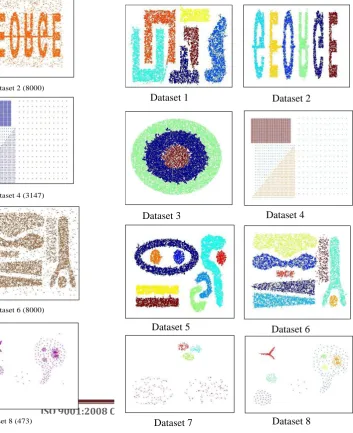
Finally, in eighth data set that contains clusters of variant densities in addition to three high densely clusters involved in large intermediate density cluster. The size of these data sets ranges from 383 to 24000 points, and their exact sizes are indicated in Fig.5.

The clustering results for the eight datasets in Fig.5 are shown in Fig.6. Different colors are used to indicate the clusters. The very small clusters are discarded as noise. It can be seen from Fig.6 that triangular and rectangular clusters are discovered and extracted based on differences in densities although they are not separated by sparse regions. This is will be more clearly when we compare the result of dataset 4 in Fig.6 with Fig.2 that result from the DBSCAN algorithm.

Dataset 1 (8000) Dataset 2 (8000)

Fig -5: Datasets used to evaluate the algorithm and

their sizes

Dataset 1 Dataset 2

Dataset 3 Dataset 4

Dataset 5 _{Dataset 6}

Dataset 7 Dataset 8

[image:6.595.39.295.350.789.2] [image:6.595.185.539.364.798.2]

(7)

[image:7.595.55.550.422.815.2]

clusters in datasets 3 and 4, where there is no separation between the clusters which having varying densities. Also it discovers the right clusters in datasets 7 and 8. We concentrate on these four datasets because they contain clusters of varying densities.

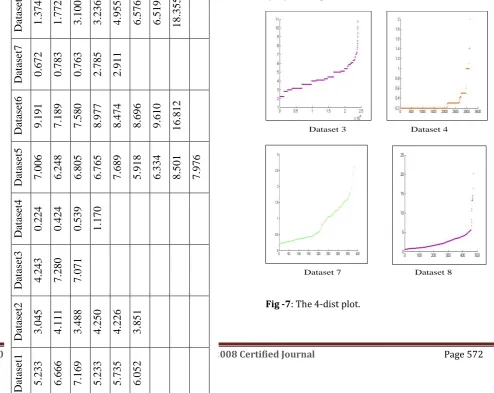
Table 1 shows the exact value for the Eps in each cluster

according to the Maxpts-distance of the starting point in each one. We can’t determine these accurate values from k-dist plot as stated in [8]. The following Fig. 7 presents the 4-dist plot for some datasets that have clusters of varying densities. Examining this Figure, we should select values that cluster dataset 3 into more than three clusters. For dataset 7 it is very difficult to determine from the k-dist plot the values that cluster it correctly, and this is the same situation for dataset 8.

6. CONCLUSION

In this paper, we have introduced a simple idea to improve the results of DBSCAN algorithm by detecting clusters with variance in density without requiring the separation

between clusters. The Minpts is fixed to 4 as in traditional

DBSCAN. The proposed algorithm requires only one input

parameter (Maxpts) that specifies the maximum number

of points around a core point; in other word, it specifies maximum level of density for a core point. And the

difference between Maxpts and Minpts represents the

allowed level of density difference inside the cluster. The

time complexity of the algorithm remains O(n log n). The

experimental results are the evidence on the efficiency of

the proposed algorithm.

D

at

as

et

8

1.374

1.772

3.100

3.236

4.955

6.576

6.519 _18.355

D

at

as

et

7

0.672

0.783

0.763

2.785

2.911 D

at

as

et

6

9.191

7.189

7.580

8.977

8.474

8.696

9.610 ₁

6.812 D

at

as

et

5

7.006

6.248

6.805

6.765

7.689

5.918

6.334

8.501

7.976 D

at

as

et

4

0.224

0.424

0.539

1.170 D

at

as

et

3

4.243

7.280

7.071 D

at

as

et

2

3.045

4.111

3.488

4.250

4.226

3.851 D

at

as

et

1

5.233

6.666

7.169

5.233

5.735

6.052 Eps1

Eps2

Ep

s3

Eps4

Eps5

Eps6

Eps7

Eps8

Eps9

Ta bl e -1 : the dif fe re nt va lue s for E ps in e ac h da ta se t a cc or di ng to the M ax pts -dista nc e of the s ta rt in g poi nt in ea ch c lus te r

Dataset 7 Dataset 8 Dataset 3 Dataset 4

[image:7.595.315.549.431.750.2]

(8)

ACKNOWLEDGEMENT

First of all thanks for Allah, then thanks for my wife, and colleagues encouraging me doing scientific research, my deep thanks for Sattam bin Abdulaziz University allowed me to use Saudi Digital Library and get the most recent papers in field.

REFERENCES

[1] M. Ankerst, M. Breunig, H.P. Kriegel, and J. Sandler.

“OPTICS: Ordering Points to to Identify the Clustering Structure”. Proceedings of the Int. Conf. on Management of Data (SIGMOD'99), 1999, pp. 49-60.

[2] B. Borah, and D.K. Bhattacharyya, “DDSC: A Density

Differentiated Spatial Clustering Technique.” Journal of Computers, Vol. 3, No. 2, February 2008, pp. 72-79.

[3] B. Borah, and D.K. Bhattacharyya, “An Improved

Sampling-Based DBSCAN for Large Spatial Databases.” proceedings of International Conference on Intelligent Sensing and Information, 2004, pp. 92-96.

[4] M. Ester, H. P. Kriegel, J. Sander, and X. Xu, “A density

based algorithm for discovering clusters in large spatial data sets with noise.” in 2nd International Conference on Knowledge Discovery and Data Mining, 1996, pp. 226–231.

[5] M. Fawzy, A. Badr, M. Reda, and I. Farag, " DBCLUM:

Density-based Clustering and Merging Algorithm.", International Journal of Computer Applications,79, 2013, pp. 1-6.

[6] A. Hinneburg and D. Keim, “An efficient approach to

clustering in large multimedia data sets with noise.” in 4th International Conference on Knowledge Discovery and Data Mining, 1998, pp. 58–65.

[7] G. Karypis, E. H. Han, and V. Kumar, “CHAMELEON: A

Hierarchical Clustering Algorithm Using Dynamic Modeling.”, Computer,32, 1999, pp. 68-75.

[8] P. Liu, D. Zhou, and N. Wu, “VDBSCAN: Varied Density

Based Spatial Clustering of Applications with Noise.”, International Conference on Service Systems and Service Management (ICSSSM), 2007, pp.1-4

[9] C-F. Tsai, and C-W. Liu, “KIDBSCAN: A New Efficient

Data Clustering Algorithm.”, ICAISC, 2006, PP. 702-711.

A Clustering Algorithm for Discovering Varied Density Clusters