CLASSIFYING ARABIC TEXT USING DEEP LEARNING

(1)

3462

PARTICLE SWARM OPTIMIZATION AND SIMULATED

ANNEALING TO DESIGN BANKRUPTCY PREDICTION

NEURAL NETWORK

1_{FATIMA ZAHRA AZAYITE,} 2_{SAID ACHCHAB}

1_{National School for Computer Science and Systems analysis, Mohammed V University, Rabat, Morocco} 2_{National School for Computer Science and Systems analysis, Mohammed V University, Rabat, Morocco}

E-mail: 1_{[email protected],}2_{[email protected]}

ABSTRACT

Bankruptcy prediction models are one of the most interesting subjects in financial engineering research, especially for investors and creditors. In this paper, the Artificial Neural Network is explored as a powerful tool to predict firms’ failure. However, defining the appropriate topology with a suitable set of parameters can be treated as an optimization problem

In this study, we investigate the use of Particle Swarm Optimization and Simulated Annealing to develop a performant learning algorithm. The proposed learning algorithm uses an evolved Particle Swarm Optimization algorithm to ameliorate the convergence of the standard algorithm and Simulated Annealing to escape from local minima. Moreover, the leaning algorithm evolves at the same time the number of hidden neurons and the weight values to design the optimum topology.

A comparative performance study with Multiple Discriminant Analysis as well as Classification and Regression Tree is reported. The results showed that the proposed model performs better in predicting firms’ Bankruptcy.

Keywords: Particle Swarm Optimization, Simulated Annealing, Artificial Neural Networks, Machine Learning, Bankruptcy

1. INTRODUCTION

This guide In recent years, the number of Moroccan bankrupt firms is in perpetual growth. This is mainly due to a difficult macroeconomic ecosystem and a competitive business environment. The effects of failure are very critical and can even be disturbing for all concerned: shareholders, employees, lenders, customers and the economy in general. The distressing effect and the current increasing number of failing firms confirm the utility of developing models to predict firms’ financial situation.

To predict financial distress, various models can be implemented based on mathematical, statistical or intelligent techniques. The first bankruptcy prediction models were made by Beaver [1] and Altman [2]. They were focused on designing models to discriminate between bankrupt and healthy firms based on statistical techniques especially Discriminate Analysis. With the appearance of Artificial Intelligence (AI), many

researchers have been interested to use these techniques because of their capability to learn from experience.

In this paper, we are interested to use one of the most performer AI models which is Artificial Neural Network (ANN). This model as a classification tool, is explored in many fields as facial recognition, medical diagnosis, and especially in bankruptcy prediction. This is due to its high classification and generalization capabilities and its ability to learn nonlinear mappings between inputs and outputs.

(2)

ISSN: 1992-8645 www.jatit.org E-ISSN: 1817-3195

3463 the first step consists of selecting the best architecture according to the problem to solve. That means fixing the number of inputs, hidden and output neurons. In many kinds of research, these parameters are chosen by experience [3] [4] [5]. but in last years, some researchers inspect the use of some metaheuristic algorithms as Genetic Algorithms (GA), or Particle Swarm Optimization (PSO) to search an optimal solution through a space of potential architectures, considering a fitness criterion. The second step which is called learning algorithm consists of finding optimum weights that perform the ANN architecture using a training model. The most known algorithm to train a Feed forward neural network is Back propagation algorithm. whereas the major limit of this algorithm is the convergence to local minima. For this reason, some researchers investigate the use of Metaheuristic algorithms as PSO and Simulated Annealing (SA) as alternative to escape local minima and search for global minima.

Taking into consideration, the good capability of optimization of PSO and the ability of SA to explore new solutions, the main goal of this paper is to investigate the use of a new hybrid learning algorithm based on PSO and SA to design an optimal ANN topology. Furthermore, we are interested to evolve the convergence of the standard PSO by introducing a new parameter that considers bad experiences in particles move. We examine through this improved PSO, the hypothesis that learning is a process based not only on good experiences but also on bad experiences.

The proposed algorithm is inspired from Zhang and Shao’s methodology [6] and uses PSO as number of hidden neurons optimization process interleaved with a second optimizing weight values based on hybrid improved PSO and SA.

In this paper, the objective is exploring the use of PSO and SA to design ANN topology. The proposed methodology evolves at the same time the number of hidden neurons and the weight values to define the optimum ANN. Moreover, an improved PSO is presented. To evaluate the proposed model, we compare its performance with Multiple Discriminant Analysis and Classification and Regression Tree. In order to validate results, comparison is made for a period of one to three years before the bankruptcy.

The rest of paper is organized as follows: Section 2 presents the basic concepts related to bankruptcy prediction and Artificial Neural Networks. In Section 3, the proposed learning algorithm is

detailed based on an evolved PSO and SA. Section 4 presents the methodology to design ANN. Section V presents the empirical findings. Finally, in Section 5, we draw some conclusions.

2 BANKRUPTCY PREDICTION WITH

NEURAL NETWORKS 2.1 Bankruptcy prediction

As Marco [1] has pointed in his review study, the firms’ bankruptcy has long been recognized for its destructive effects on the economy and society. Since the 20th century, many kinds of research followed [2] [3] treating the subject in various aspects: economic, financial, strategic and organizational.

The definition of the bankruptcy is complex and depends on the angle of observation of the phenomenon. There are several definitions of the concept of failure as highlighted by Karels and Prakash [4]. However, in this paper, the definition adopted is a legal definition. Bankruptcy is declared when the firm is no longer able to meet its financial obligations [5] as salaries, suppliers’ payment or banks’ credits and then engages legal procedure of liquidation.

To avoid the negative effects of a bankruptcy, Various researchers are interested in predicting the legal failure by designing predictive models that separate between failing and non-failing firms based on an appropriate set of financial variables. In literature, these models are categorized into two classes [6, 7, 8]: statistical models and Machine Learning models. The statistical models are the most known and the first used to predict failure. Early studies are made by Beaver [5] and Altman [2] and they are based on single and multiple discriminant analysis.

(3)

3464 Artificial Neural Networks to predict bankruptcy and demonstrate their high predictive capabilities compared to statistical models. Various studies followed comparing the performance of the ANN to other models: the study developed by Lin [17] examined the predictive ability of the four most commonly used bankruptcy prediction models namely Multiple Discriminant Analysis (MDA), logistic regression (Logit), binomial regression (Probit) and Artificial Neural Networks (ANN). The results show high performances of the ANN approach with a better rate of correct classification the available data do not respect the requirements of the statistical approach. Also, Tsukuda and Baba [18] compared the failure prediction performance of Artificial Neural Network and Multiple Discriminant Analysis for a period of one to three years before the bankruptcy. The experiment made with two different samples of companies demonstrated the high performance of neural networks in the presence of noisy data. Ruibin Geng [19] also concluded that Artificial Neural Networks perform better in comparison to other classifiers, such as Decision Trees, Support Vector Machines, and a set of multiple classifiers combined. Azayite and Achchab [20] studied the performance of a hybrid discriminant analysis and artificial neural networks to predict firms’ distress. The results demonstrate that the proposed approach is much accurate than the conventional neural network approach.

All these studies demonstrate the utility of using ANN to predict bankruptcy. So, in the next section, we are interested to define ANN, its parameters and constraints that should be considered to design a bankruptcy prediction model.

2.2 Artificial Neural Networks for pattern classification

Defined as a branch of Artificial Intelligence, ANN can build machines capable of learning and performing specific tasks like classification, prediction or clustering. The human neuron is at the origin of the Artificial Neural Networks theories. The network component describes the organization of these neurons which are interconnected according to architecture.to understand how ANN works, we start by defining how biological neuron, the original unit for artificial neuron, works.

A biological neuron is a living elementary cell with the ability to process information locally and then transmit it to neurons connected. This cell has the faculty of learning through the change of the intensity of its connections with the attached neurons as well as its treatment rules. This change

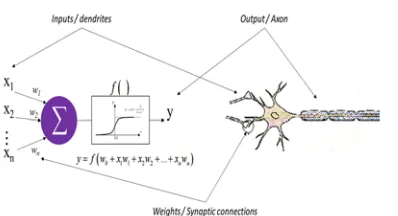
is the fundamental principle of neuron behavior. The neuron receives signals in the form of electrical impulses through the dendrites and sends the information through the axons. The connections between two neurons (between axon and dendrite) are via synapses. Figure 1 shows a representation of the biological neuron as well as the similarity to the artificial neuron.

The artificial neuron is the elementary unit in an ANN. It can do only simple operations: It receives several input variables xi from neurons directly connected. These connections are associated with weights wi which translate their strength. It is

generally composed of the following elements: • One or more entries i with a value xi .

• Weights wi .

• A transfer function f() as the threshold function, the sigmoid function, etc.

• An output y.

As shown in Fig 1, the weights correspond to the synaptic connections, the transfer function corresponds to the cell body which processes the input signals and the output of the neuron has the similar function of the axon which transmit the calculated output to the next neuron.

A neuron can be represented mathematically by a multivariate function with a single output. The equation can be described by:

𝑦 𝑓 𝑤 ∑ 𝑤 ∙ 𝑥 (1) With n is the number of inputs.

The topology of an Artificial Neural Network plays a fundamental role in its behavior. A multilayer network is commonly used, and it’s composed with an input layer, output layer and one or more hidden layers that define the mapping between input neurons xi and output neurons yz.

[image:3.612.324.523.100.208.2]

The relationships between neurons are stored as

(4)

3465 weights. The layers are usually interconnected in a feed-forward way that means information moves in the only forward direction, from the input nodes through the hidden nodes, to the output nodes with no cycles or loops in the network. In literature, ANN with one hidden layer is the best structure to use for classification problems [12]. For this reason, this structure is adopted in this paper.

In the case of a feedforward ANN with a single hidden layer, each hidden neuron j = 1, ..., m, receives an input equal to the weighted sum of the inputs of the network then applied a transfer function f to transform input signal to an output signal defined in equation (2)

(2)

with n and m are respectively the number of input and hidden neurons, wji is the weight from the

ith_{input neuron to the j}th_{hidden neuron, xi is input}

variable i and wj0 is a bias term.

With similarity to what happens between input and hidden layer, the signals from the hidden neurons are then sent to output neurons through weighted connections. As a result, the output nodes receive the sum of all weighted hidden neurons with an applied transfer function g depending on the desired output interval. The output yo of the output

neuron o of the network is then formulated by:

(3)

With zj is the weight from the jth hidden neuron

to the oth_{output neuron and b}_z0_{is a bias term.}

ANN are used in various domains and it’s due to their ability to approximate any linear and non-linear function. Therefore, defining the appropriate topology to predict failure is one of the challenging tasks: there are parameters that must be optimized when designing an ANN:

The number of input neurons represents the number of input variables. In the case of bankruptcy prediction, the main goal is to separate between healthy and bankrupt firms based on some financial variables. So, the input neurons denote the financial variables that can make the ANN learn from examples to classify new features. Consequently, it

is important to define variables that are the most relevant to do so. As mentioned by F. Du jardin [21] a neural-network-based model for predicting bankruptcy performs significantly better when designed with variable selection techniques than when designed with methods generally used in the financial literature. For this purpose, we use variables selection models to define appropriate financial and save money and effort for collecting and validating Data.

The number of hidden neurons is another parameter that should be fixed in an ANN topology. It is a challenging task: If there are too many neurons, the number of possible computations that the algorithm has to deal with increases. Otherwise, choosing a few nodes in the hidden layer can reduce the learning ability of the model [22]. So, it’s very important to select the appropriate number of hidden neurons that can maximize network performance.

As mentioned before, weight values are parameters that allow the ANN to mimic a specific behavior. These parameters are generally fixed by a learning algorithm. The learning algorithm is usually an iterative process containing a set of rules to find optimum values of weights and biases that maximize the neural network performance. In this paper, we propose a learning algorithm that evolves at the same time the number of hidden neurons as well as the weight values. This algorithm is based on an improved PSO and SA.

3 EVOLVED PSO AND SA TO TRAIN AN ANN

As mentioned before, ANN can be a powerful classification tool if it is designed with appropriate variables. However, defining the optimum ANN topology according to the problem to solve can be seen as an optimization problem. In this paper, we are interested to explore PSO and SA capabilities to build a learning algorithm. Our goal through the proposal of this new algorithm is:

• the improvement of the performance of the standard PSO learning algorithm by presenting an improved PSO.

• Escape local minima and search for global minima by introducing SA as a trial way. • Evolves at the same time the number of

(5)

3466 Before presenting the proposed algorithm, we start by presenting the standard PSO et SA.

3.1 Particle Swarm Optimization (PSO)

Described as a metaheuristic algorithm, PSO is one of the swarm intelligence algorithms that are inspired by the natural process of social behavior of organisms. It is an algorithm developed in 1995 by a social psychologist J. Kennedy and an electrical engineer R. Eberhart [23]. It is applied in many research areas as a powerful optimization technique and it is known to have good exploitation capabilities in a solution space compared to traditional algorithms. In the PSO algorithm, the potential solutions, called particles, fly through the problem solutions space by following the current optimum particles.

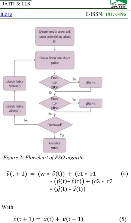
So, to apply PSO, it is needed to define the search space composed of particles and a fitness function to optimize. As summarized in the flowchart presented in Figure 2, the system is initialized with a population of random particles. Each particle has a position value representing a possible solution, a velocity value indicating how much the Data can be changed as formulated in equation (4) and a personal best value (pBest) representing the best solution reached by the particle.

The particle velocity is influenced by three components:

• Physical component w ∗ 𝑣⃗ t ; the particle tends to follow its own path through the vector

• Cognitive component c1 ∗ r1 ∗ p⃗ t – 𝑥⃗ t ; it tends to return to the best position by which it has already passed through the vector

• Social component c2 ∗ r2 ∗ 𝑔⃗ t – 𝑥⃗ t ; it tends to move towards the best position already reached by its neighbors through the vector

With w is an inertia weight, v velocity of the particle in the iteration t, c1 and c2 are respectively cognitive and social parameters, r1 and r2 random numbers between 0 and 1, p the particle best position (pBest), x the particle current position and g the swarm best position (gBest).

So, the equation to update velocity of the particle is defined as follows:

𝑣⃗ t 1 w ∗ 𝑣⃗ t c1 ∗ r1

∗ 𝑝⃗ t – 𝑥⃗ t c2 ∗ r2

∗ 𝑔⃗ t – 𝑥⃗ t

(4)

With

𝑥⃗ t 1 𝑥⃗ t 𝑣⃗ t 1 (5)

3.2 Simulated Annealing (SA)

Simulated Annealing is a stochastic algorithm introduced by Kirkpatrick [24]. It is inspired by the physical process of metal annealing where it is heated up very strongly and then cooled gradually to get into a perfect state using a minimum of energy. This process is assimilated to an optimization: By analogy, the physical states of the material, the energy, and the temperature correspond respectively to the solutions of a problem, the cost of a solution and a control parameter.

[image:5.612.311.528.55.425.2]

In the search process, SA accepts not an only best but also worse solution with a probability. At the beginning of the process, the temperature is high and the probability of accepting a worse solution is also high but as the temperature is decreasing, the probability of a worse solution acceptance gradually approaches zero. Starting from a random initial solution, for each iteration objective function E is calculated and compared with the previous value. If the new objective function value is better, the new solution is automatically accepted otherwise can be accepted with a probability formulated in equation (6).

(6)

3467

𝑃 e / ₍₆₎

with T the current temperature. This mechanism allows exploring new space of solutions either better or worse. This property can be used as a trial way to leave local minima.

3.3 Improved PSO and SA to design the ANN topology

In many researches based on ANN to predict failure, learning algorithms are employed to find only optimal weights. The number of hidden neurons is generally chosen by experience [25] [26] [14].

One of the main objectives of this work is to propose a learning algorithm able to search for the same time the optimal architecture and the connection weights for better performance. For this reason, we focused on the exploitation of evolutionary algorithms inspired by social behavior in a community and more specifically the Particle Swarm Optimization algorithm. for learning neural networks.

Inspired by the methodology of Zhang and Shao (Zhang, et al., 2000), we develop an approach based on two loops interconnected:

• External loop: Contains an algorithm that is

used to optimize the ANN architecture and specially the number of hidden neurons to use.

• Internal Loop: It is interleaved into the first

loop and it is used to optimize the weight values for each architecture presented by the first loop.

The optimum solution concerns the ANN that gives the best results according to performance measures. In this paper, the algorithm developed as detailed is Algorithm1, is composed of PSO as the external loop and the proposed algorithm as the internal loop whereas the internal loop is a combination of an evolved PSO and SA. Our goal through the proposal of this new algorithm is the improvement of the performance of the standard PSO learning algorithm.

The evolved PSO algorithm is based on the hypothesis that learning is a process-based not only on good experiences but also on bad experiences. For this reason, the initial equation of velocity presented in equation (4) was modified by introducing a new parameter pWorse which

corresponds to the last negative point reached by the particle (equation 7). The velocity is then calculated as follows:

𝑣⃗ t 1 w ∗ 𝑣⃗ t c1 ∗ r1

∗ 𝑝⃗ t – 𝑥⃗ t c3 ∗ r3

∗ 𝑝𝑊𝑜𝑟𝑠𝑒⃗ t – 𝑥⃗ t c2 ∗ r2 ∗ 𝑔⃗ t – 𝑥⃗ t

(7) 1. For each particle in swarm S- the population of

architectures A 2. Initialize particle

3. Create network with a random n hidden neurons 4. End

5. While stopping condition 1 is false do 6. For each particle Ai of the swarm A do

7. //execute PSO algorithm (Ai weights)

8. Generate particles swarms Bj with random weights matrix as position.

9. While stopping condition 2 is false do 10. For each particle j of the swarm do 11. Calculate the fitness f(xj(t));

12. If the fitness value >pBest(j) // if it is the best solution

13. Set current value as the new pBest(j) 14. Else // apply SA in worse solutions 15. Compute ΔE = fitness f(xj(t)) - the fitness

f(xj(t-1))

16. Probability = exp(-ΔE/KT)

17. If Probability > random number between 1 and 0

18. Accept the worse solution set current value as the new pWorse(j)

19. End

20. End for

21. t = frac * t; // frac < 1// Lower the temperature for next cycle

22. w= r * w ; // r<1 changing inertia

23. Choose the best fitness value of all the particles in B swarm as gbest(B)

24. For each particle j of the B swarm do

25. Update particle j velocity according equation (4) 26. Update particle j position according equation (5) 27. End for

28. End while

29. Fitness value = gBest(B); 30. If the fitness value >pBest(A)

31. Set current value as the new pBest(A)

32. End

33. End for

34. Choose the best fitness value of all the particles as gBest

(7)

3468 The introduction of the value of the last negative point reached in the behavior of the particle provides additional information in the cognitive component. The vector of the bad experience allows the particle to move away from its last negative point and try to find the best solution. Also, in this algorithm, the w inertia value is changed linearly for each iteration.

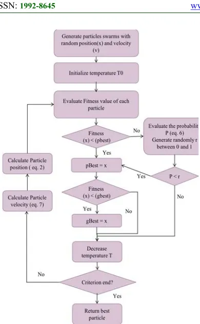
This evolved algorithm is combined with Simulated Annealing which is introduced as a trial way to explore new solutions either better or worst in the defined search area. As the purpose of SA is accepting a worse solution according to a probability that gradually decreases as the temperature decreases to approach zero, this technique allows jumping out from local minima. The flowchart of the hybrid algorithm is presented in Figure 3.

4 DESIGNING ARTIFICIAL NEURAL

NETWORK TO PREDICT

BANKRUPCTY

In this paper, the main goal is to design an optimum topology of an ANN using a proposed learning algorithm. For this propose the

methodology adopted should consider three important questions:

• What are the appropriate variables to consider predicting bankruptcy?

• With this particular Data Set, what is the optimum topology of a neural network that defines the relationship between the relevant financial variables and the likelihood of bankruptcy?

• How can we evaluate the performance of the proposed neural network in predicting bankruptcy?

For the first question, there is no financial ratios set communally used in the literature to use as early warning indicators to predict failure. As there is a large number of possible financial ratios, the methodology should consider an approach to define the relevant ones. For the second question, the proposed learning algorithm is tested exploring the PSO and SA capability. This algorithm evolves at the same time the number of hidden neurons and the weight values to define the optimum ANN. The proposed model should identify the firms’ health with a high accuracy. For the last question, to evaluate the proposed algorithm, minimize the bias effect and avoid over fitting, a four cross validation technique is applied. The methodology adopted is presented in Fig. 4 and detailed below.

4.1 Financial variables to predict bankruptcy In the process of building a neural networks-based model, the first step is the definition of the learning Data, which must reflect as accurately as possible the knowledge to extract and to develop by the classification model. This task, which conditions the functionally and the performance of the model, is complicated.

On the one hand, there is no financial ratios list communally used in the literature to predict the financial situation of companies and there is a large number of variables that can be used for this purpose. According to the Bellovary survey [27] based on the comparison of Six hundred and seventy-four studies, the number of financial ratios considered in each study varies from one to fifty-seven ratios. A total of 752 separate ratios were used in these studies and are used in only one or two studies.

[image:7.612.95.290.73.389.2]

On the other hand, F. Du Jardin [21] has demonstrated that a prediction model based on an Artificial Neural Network is much more efficient when it is designed with appropriate variable selection techniques rather than designed with

(8)

3469 methods commonly used in the literature. So, before defining a bankruptcy prediction model, it’s essential to define the most relevant variables specially when we have many variables as inputs. To do so, it is recommended to use variable selection techniques.

Variable selection model is a process that determines a subset of M variables from an initial

set N (M<N) according to some criteria [28] . Lui and Motoda [29] have pointed out that selecting variables for the purpose of Machine Learning allows to:

 Reduce the dimensionality of the space of the variables,

 Accelerate the learning process

 Improve the prediction of classification algorithms

 Improve the interpretation of the results. To define the initial set of financial ratios, we took into account results obtained by Azayite and Achchab [30] where authors proved the importance of variables selection models to select appropriate input variables especially in a context of missing data. They concluded that the use of variables selection models shows a high performance mainly Decision trees models to define neural networks inputs.

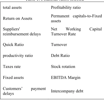
[image:8.612.55.511.59.361.2]

So, financial ratios used in this paper are the relevant variables selected by the union of two Decision Tree algorithms which are Classification and Regression Tree and Chi-squared automatic interaction detector. The list of variables is summarized in Table 1.

Figure 4: Methodology proposed

Table 1: Financial ratios selected

total assets Profitability ratio

Return on Assets Permanent capitals-to-Fixed _assets

Suppliers'

reimbursement delays

Net Working Capital Turnover Rate

Quick Ratio Turnover

productivity ratio Debt Ratio

Taxes rate Stock rotation

Fixed assets EBITDA Margin

Customers’ payment

[image:8.612.84.302.505.715.2]

(9)

3470 Data preprocessing consists of cleaning, correcting and processing the data to improve their quality and prepare them to be consumed by an ANN model.

4.2 Cross validation and performance evaluation

Cross-validation is a technique used when the data available to prepare the training and test sets are limited. The principle is to reserve a percentage of data for the test, and the rest is used for training and exchanging after the role of each of the partitions. This technique is introduced to minimize the bias effect.

In this study, a 4-fold cross-validation technique is used to avoid over fitting. That means, data set is randomly split into 4 mutually exclusive subsets of approximately equal sizes and the model is trained and tested 4 times: Each time, the model is trained on 3 folds and tested on the remaining 1-fold. The overall accuracy of a model is evaluated by averaging the 4 individual accuracy measures

We are interested to evaluate the performance of the proposed bankruptcy prediction model. This model is built using a sample of companies whose health status (Bankrupt or healthy) is known to extract knowledge and then classify new companies. This leads us to say that the criterion of the performance is the generalization capacity of the model. This can be measured by evaluating the gap of the health predictions based on the test data set using the formula of the Mean Squared Error:

MSE 1

n t y (8)

with yi calculated output, ti desired output and n

number of observations.

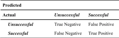
However, this information may be insufficient. In the case of two-class classification problems, the result obtained from the model is either positive in the case of a correct classification, or negative in

the case of an incorrect classification. The calculated error rate in this case does not distinguish the classification errors in each class. But the cost of error can differentiate from one class to another: A misclassification of a bankrupt firm by a predictive model can be very expensive for a lander than a misclassification for a healthy company. For this reason, classification rates have been established based on the distinction of the four possible classification cases formulated in a matrix called confusion matrix (Table 2). To define the percentage of records that are correctly predicted by a model, a metric called Overall accuracy or correct classification is calculated. Its formula, according to confusion matrix in Table 2 is:

Correct classification TP TN

TP TN FP FN

4.3 Comparison and results validation

In order to validate the performance of the ANN based model, a comparison with other techniques is made. In this paper, the results are compared with the two popular models to predict failure: C&RT and DA.

C&RT (Classification and regression tree) is a binary decision tree algorithm that was established by [5]. It’s an algorithm that works recursively to split data into two subsets to make records in each subset more homogeneous than the previous. The subsets are again splinted until the homogeneity criterion or other stopping criteria are satisfied. In this method, the same predictor variable can be used many times in the tree. The final aim of splitting is to determine the right variable with the right threshold to maximize the homogeneity of the sample subgroups.

MDA (Multiple Discriminant Analysis) is a statistical technique. It is used to find a linear combination of features that characterizes or separates two or more classes of objects or events and, more commonly, for dimensionality reduction before later classification. In this research, we used a stepwise method applying Wilk’s Lambda to select sequentially significant variables from the set of variables.

[image:9.612.93.300.112.179.2]

Moreover, the proposed model is compared with a neural network-based model trained with the standard PSO interleaved with another PSO to validate the proposed evolved PSO.

Table 2: Confusion matrix

Predicted

Actual Unsuccessful Successful

Unsuccessful True Negative False Positive

(10)

3471

5 EXPERIMENTATION AND RESULTS

For the experiment, the database used contains financial ratios for a sample of Moroccan firms. Data collected concerns 792 companies’ balanced 50% bankrupt firms and 50% healthy firms. A binary variable is created with two values (0 if it is failed and 1 if it is healthy).

As mentioned before, the financial ratios used as input variables are presented in Table I and selected as relevant variables by a variable selection technique. These sixteen variables represent the input for the ANN, C&RT and MDA in order to build a predictive model. Before using Data as input, we normalized it to bound data values between -1 and +1.

For ANN, the model is trained first with the standard PSO-PSO based on two loops interleaved of PSO according to the Zhang and Shao’s methodology [6].

The second ANN is trained with the proposed learning algorithm based on two loops: PSO and improved PSO and SA to design its topology. In order to minimize the bias effect and avoid over fitting, a four cross validation technique is applied.

To use the algorithms based on two loops of PSO as presented before, we used the parameters below:

PSO for architectures optimization: • Swarm size (s = 20) and stop criteria (15

iterations)

• Search space limit [7, 30]

• Inertia factor (wn= 0.9 wn-1, w0= 0.8)

• Acceleration factors (c1 = c2 = 1.4960) Improved PSO for weights optimization: • Swarm size (s = 50) and stop criteria (100

iterations)

• Search space limit [−2.0, 2.0] • inertia factor (wn= 0.9 wn-1, w0= 0.8)

• Acceleration factors (c1 = c2 = 1.4960)

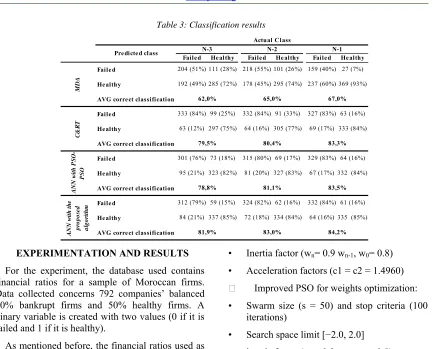
The results, presented in Table 3, revealed that the average of correct classification rate through 3 years for respectively MDA, C&RT, ANN with PSO-PSO and ANN with the proposed learning algorithm is respectively 65%, 81%, 81 and 83%.

For the three horizons predicted, the proposed model showed the best average correct classification with 81.9%, 83% and 84.2% for three, two- and one-year time horizon. Therefore, it outperforms the standard PSO-PSO which means considering information about bad experiences ameliorates the PSO performance. Also, we can observe for the three models that the accuracy deceases as the time horizon increases.

[image:10.612.95.536.82.431.2]

In order to analyze the importance of variables introduced in the ANN model, we use Garson index [33]. For this purpose, we applied Garson index to ANN model created to predict bankruptcy one year before where the accuracy is higher. The indexes used are 16 corresponding to number of input variables of each model. Figure 5 shows the percentage weight of each variable in predicting

Table 3: Classification results

Failed Healthy Failed He althy Failed Healthy Faile d 204 (51%) 111 (28%) 218 (55%) 101 (26%) 159 (40%) 27 (7%)

Healthy 192 (49%) 285 (72%) 178 (45%) 295 (74%) 237 (60%) 369 (93%)

AVG correct classification

Faile d 333 (84%) 99 (25%) 332 (84%) 91 (33%) 327 (83%) 63 (16%)

Healthy 63 (12%) 297 (75%) 64 (16%) 305 (77%) 69 (17%) 333 (84%)

Faile d 301 (76%) 73 (18%) 315 (80%) 69 (17%) 329 (83%) 64 (16%)

Healthy 95 (21%) 323 (82%) 81 (20%) 327 (83%) 67 (17%) 332 (84%)

Faile d 312 (79%) 59 (15%) 324 (82%) 62 (16%) 332 (84%) 61 (16%)

Healthy 84 (21%) 337 (85%) 72 (18%) 334 (84%) 64 (16%) 335 (85%)

Predicte d class N-3 N-2 N-1

Actual Class

65,0% 67,0%

79,5% 80,4% 83,3%

81,1% 83,5%

81,9% 83,0% 84,2%

MD

A

C&

RT

A

NN w

it

h

P

S

O-PS

O

A

N

w

ith

th

e

pr

opos

e

d

al

gor

it

h

m

(11)

3472 bankruptcy. We can observe that turnover and profitability ratios are the most influent variables with 22% and 16%. These results are on accordance with financial analysis because these two ratios provide an indication of the firm’s profitability, cost structure, solvency and its capability of generating liquidity.

CONCLUSION

Considering the importance of defining appropriate ANN topology to predict bankruptcy, we analyze in this paper the use of the Particle Swarm Optimization and Simulated Annealing to develop a performing learning algorithm.

The proposed learning algorithm uses an advanced PSO to ameliorate the convergence of the standard PSO and SA to escape from local minima. Moreover, it evolves at the same time the number of hidden neurons and the weight values to define the optimum ANN. The methodology adopted considers also data availability constraints by using variable selection techniques to define relevant financial variables.

Artificial Neural Network trained with the proposed learning algorithm and the relevant variables shows better mean generalization performance compared to MDA and C&RT for a period of one to three years before the bankruptcy even in the context of missing data. These results prove that learning is a process-based not only on good experiences but also on bad experiences. REFERENCES

[1] L. Marco, La montée des faillites en France XIXe-XXe siècles, 1 éd., Editions l'Harmattan, 1989.

[2] E. Altman, «Financial ratios, discriminant analysis and the prediction of corporate bankruptcy,» Journal of

Finance , 1968.

[3] R. C. Morris, Early warning indicators of corporate failure : a critical review of previous research and further empirical evidence, Ashgate, 1997.

[4] G. V. Karels et A. J. Prakash, «Multivariate Normality and Forecasting of Business Bankruptcy,» Journal of

Business Finance and Accounting, vol.

14, n° %114, pp. 573-593, 1987.

[5] W. H. Beaver, «Financial Ratios as Predictors of Failure,» Journal of

Accountant Research, 1966.

[6] T. Korol, «Early warning models against bankruptcy risk for Central European and Latin American enterprises,» Economic

Modelling, vol. 31, n° %1march, pp.

22-30, 2013.

[7] J. H. Min et C. Jeong, «A binary classification method for bankruptcy

prediction,» Expert Systems with

Applications, vol. 36, pp. 5256-5263 ,

2009.

[8] H. Li et J. Sun, «Empirical research of hybridizing principal component analysis with multivariate,» Expert Systems with

Applications, n° %138, p. 6244–6253,

2011.

[9] C. V. Zavgren, «Assessing the vulnerability to failure of american industrial firms: a logistic analysis,»

Journal of Business Finance and

Accounting, pp. Volume 12, 19-45, 1985.

[10] M.-Y. Chen, «Bankruptcy prediction in firms with statistical and intelligent techniques and a comparison of evolutionary computation approaches,»

Computers and Mathematics with

Applications, vol. 62, pp. 4514-4524,

2011.

[11] F. M. Rafiei, S. Manzari et S. Bostanian, «Financial health prediction models using artificial neural networks, genetic,»

Expert Systems with Applications, vol.

38, p. 10210–10217, 2011.

[12] J. H. Min et Y.-C. Lee, «Bankruptcy prediction using support vector

machine,» Expert Systems with

[image:11.612.225.519.62.727.2]

Applications, p. 603–614, 2005.

(12)

3473 [13] X. Xu et Y. Wang, «Financial failure

prediction using efficiency as a

predictor,» Expert Systems with

Applications, vol. 36, pp. 366-373, 2009.

[14] C.-F. Tsai et J.-W. Wu, «Using neural network ensembles for bankruptcy,»

Expert Systems with Applications, vol.

34, p. 2639–2649, 2008.

[15] C. Serrano-Cinca, «Self organizing neural networks for financial diagnosis,»

Decision Support Systems, vol. 17,

n° %13, pp. 227-238, 1996.

[16] M. D. Odom et R. Sharda, «A Neural

Network Model for Bankruptcy

Prediction,» IJCNN International Joint

Conference on Neural Networks , pp. 163

- 168, 1990.

[17] T.-H. Lin, «A cross model study of corporate financial distress prediction in Taiwan: Multiple discriminant analysis, logit, probit and neural networks models,» Neurocomputing, pp.

3507-3516, 2009.

[18] J. Tsukuda et S.-i. Baba, «Predicting japanese corporate bankruptcy in terms of financial data using neural network,»

Computers & Industrial Engineering,

vol. 27, pp. 445-448, 1994.

[19] R. Geng, I. Bose et X. Chen, «Prediction of financial distress: An empirical study of listed Chinese companies using data

mining,» European Journal of

Operational Research, p. 236–247, 2015.

[20] f. z. azayite et s. achchab, «Hybrid Discriminant Neural Networks for bankruptcy prediction and risk scoring,»

Procedia Computer Science, 2015.

[21] P. du Jardin, «Predicting bankruptcy using neural networks and other classification methods: the influence of variable selection techniques on model accuracy,» Neurocomputing, 2010.

[22] D. T. Larose et C. D. Larose, Discovering knowledge in data: an introduction to data mining, Wiley, 2014. [23] R. C. a. K. J. Eberhart, «A new optimizer

using particle swarm theory.,» Vols. %1 sur %2pp. 39-43, 1995.

[24] C. D. G. J. M. P. V. S. Kirkpatrick, «Optimization by Simulated Annealing,»

Science, vol. 220, pp. 671-680, 1983.

[25] T.-S. Lee, C.-C. Chiu, C.-J. Lu et I.-F.

Chen, «Credit scoring using the hybrid neural discriminant technique,» Expert

Systems with Applications, p. 245–254,

2002.

[26] A. Roy, D. Dutta et K. Choudhury, «Training Artificial Neural Network using Particle Swarm Optimization Algorithm,» International Journal of Advanced Research in Computer Science

and Software Engineering, vol. 3,

n° %13, March 2013.

[27] J. Bellovary, D. Giacomino et M. Akers, «A Review of Bankruptcy Prediction Studies: 1930-Present,» Journal of

Financial Education, vol. 33, 2007.

[28] A. L. Blum et P. Langley, «Selection of relevant features and examples in

machine learning,» Artificial

Intelligence, vol. 97, n° %1Elsevier, pp.

245-271 , 1997.

[29] H. Liu et H. Motoda, Feature Selection for Knowledge Discovery and Data Mining, Kluwer Academic Publishers, 1998.

[30] f. z. azayite et s. achchab, «The impact of payment delays on bankruptcy prediction: A comparative analysis of variables selection models and neural

networks,» 2017 3rd International

Conference of Cloud Computing Technologies and Applications

(CloudTech), 2017.

[31] W. McCulloch et W. Pitts, A Logical Calculus of the Ideas Immanent in Nervous Activity, vol. 5, Bulletin of Mathematical Biophysics, pp. 115-133. [32] Y.-C. L. Jae H. Min, «Bankruptcy

prediction using support vector

Applications, p. 603–614, 2005.

[33] J. H. Min et Y.-C. Lee, «Bankruptcy prediction using support vector

Applications, p. 603–614, 2005.

[34] A. W. R. M. N. R. A. H. T. a. E. T. Nicholas Metropolis, «Equation of State Calculations by Fast Computing Machines,» The journal of chemical

Physics, n° %121, pp. 1087-1092, 1953.

[35] J. A. Ohlson, «Financial Ratios and the Probabilistic Prediction of Bankruptcy,»

(13)

3474 18, No. 1, pp. 109-131, 1980.

[36] I. B. X. C. Ruibin Geng, «Prediction of financial distress: An empirical study of listed Chinese companies using data

mining,» European Journal of

Operational Research, p. 236–247, 2015.

[37] A. Salappa, M. Doumpos et C. Zopounidis, «Feature Selection Algorithms in Classification Problems:

An Experimental Evaluation,»

Optimization Methods Software, vol. 22,

n° %1Issue 1, pp. 199-212, 2007.

[38] E. Fedorova, E. Gilenko et S. Dovzhenko, «Bankruptcy prediction fo Russian companies : Application of combined classifiers,» Expert Systems

with Applications, pp. 7285-7293, 2013.

[39] L. Liang et D. Wu, «An application of pattern recognition on scoring chinese corporations financial conditions based on backpropagation neural network,»

Computers & Operations Research, pp.

1115-1129, 2005.

[40] G. Kass, «An Exploratory Technique for Investigating Large Quantities of Categorical Data,» Applied Statistics,

vol. 29, n° %12, pp. 119-127, 1980.

[41] H. S. C. Zhang, «An ANN’s Evolved by a New Evolutionary System and Its application,» In Proceedings of the 39th IEEE Conference on Decision and

Control, vol. 4, pp. 3562-3563, 2000.

[42] L. Breiman, J. Friedman, C. J. Stone et R. Olshen , «Classification and Regression Trees,» 1984.

[43] G. D. Garson, «Interpreting neural-network connection weights,» AI Expert,

vol. 6 Issue 4, pp. 46 - 51, 1991.