BIROn - Birkbeck Institutional Research Online
Blackburn, S.R. and Etzion, T. and Martin, K.M. and Paterson, Maura
B. (2010) Distinct difference configurations:
multihop paths and key
predistribution in sensor networks. IEEE Transactions on Information Theory
56 (8), pp. 3961-3972. ISSN 0018-9448.
Downloaded from:
Usage Guidelines:
Please refer to usage guidelines at
or alternatively
BIROn
-
B
irkbeck
I
nstitutional
R
esearch
On
line
Enabling open access to Birkbeck’s published research output
Distinct difference configurations: multihop paths and
key predistribution in sensor networks
Journal Article
http://eprints.bbk.ac.uk/2907
Version: Post-print (Refereed)
Citation:
© 2010 IEEE
Publisher version available at:
http://dx.doi.org/10.1109/TIT.2010.2050794
______________________________________________________________
All articles available through Birkbeck ePrints are protected by intellectual property law, including copyright law. Any use made of the contents should comply with the relevant law.
______________________________________________________________
Deposit Guide
Contact: [email protected]
Birkbeck ePrints
Birkbeck ePrints
arXiv:0811.3896v2 [math.CO] 8 Oct 2009
Distinct Difference Configurations: Multihop Paths
and Key Predistribution in Sensor Networks
Simon R. Blackburn, Tuvi Etzion, Keith M. Martin and Maura B. Paterson
Abstract—A distinct difference configuration is a set of points
in Z2 with the property that the vectors (difference vectors) connecting any two of the points are all distinct. Many specific examples of these configurations have been previously studied: the class of distinct difference configurations includes both Costas arrays and sonar sequences, for example.
Motivated by an application of these structures in key pre-distribution for wireless sensor networks, we define the k-hop coverage of a distinct difference configuration to be the number of distinct vectors that can be expressed as the sum of k or fewer difference vectors. This is an important parameter when distinct difference configurations are used in the wireless sensor application, as this parameter describes the density of nodes that can be reached by a short secure path in the network. We provide upper and lower bounds for the k-hop coverage of a distinct difference configuration withmpoints, and exploit a connection with Bh sequences to construct configurations with maximal k
-hop coverage. We also construct distinct difference configurations that enable all small vectors to be expressed as the sum of two of the difference vectors of the configuration, an important task for local secure connectivity in the application.
Index Terms—Data Security, Key Predistribution, Wireless
Sensor Networks
I. INTRODUCTION
A
distinct difference configurationDD(m)is a set of m dots in a square grid, with the property that the lines joining distinct pairs of dots are all different in length or slope. For instance, the dots depicted in the following array form aDD(3):
• • •
If we pick a position on the square grid to be the origin, we may think of the dots in a DD(m)as a set{v1,v2, . . . ,vm}
of vectors in Z2. The condition that the dots form aDD(m)
is then the same as the condition that the difference vectors
vi−vj with i6=j are all distinct. So we may think of the
dots in the example above as the set{(0,0),(1,2),(2,1)} of vectors; it is easy to verify that the six difference vectors are all different in this case.
Many special classes of distinct difference configurations have been studied previously: these include B2 sequences
over Z and Golomb rulers in the one-dimensional case, and Costas arrays, Golomb rectangles and sonar sequences in the two-dimensional case. See [1] for a summary of these configurations.
This work was supported in part by EPSRC grants EP/D053285/1 and EP/F056486/1, and Israel Science Foundation grant 230/08.
S.R. Blackburn, K.M. Martin and M.B. Paterson are with the Department of Mathematics, Royal Holloway, University of London, Egham, Surrey TW20 0EX. T. Etzion is with the Computer Science Department, Technion–Israel Institute of Technology, Haifa 32000, Israel.
This paper is concerned with thek-hop properties of distinct
difference configurations. Before we explain this, we first need to discuss an application to key predistribution in grid-based wireless sensor networks due to Blackburn, Etzion, Martin and Paterson [2] that motivates our work.
A. Wireless Sensor Networks
A wireless sensor network is a large collection of small sensor nodes that are equipped with wireless communication capability. Sensor nodes have limited communication range and thus data transmitted over the network is typically passed from node to node in a series of hops in order to reach its end destination. Such networks can be employed for a wide range of applications [3], whether scientific, commercial, humanitarian or military. The data being transmitted over the wireless medium is frequently valuable or sensitive; hence, there is a need for cryptographic techniques to provide data integrity, confidentiality and authentication.
On deployment, the sensor nodes aim to form a secure and connected network. In other words, we desire a significant proportion of nodes within communication range to share cryptographic keys. The nodes’ size limits their computa-tional power and battery capacity, so it is assumed that the sensor nodes are unable to use public key cryptography to establish shared keys. So symmetric cryptographic keys are preloaded onto each node before deployment: methods for deciding which keys are assigned to a node are known as key predistribution schemes (see [4]–[6] for surveys of this subject). The sensor nodes are assumed to be highly vulnerable to compromise, so a single key should not be given to too many nodes. A balancing constraint is that each node can only store a limited number of keys. The aim is to design an efficient and secure key predistribution scheme so that a sensor node can establish secure wireless links with many of its neighbours: it is important to establish as many short secure links in the network as possible, since the nodes’ capacity to relay information is very limited.
monitoring conditions in an orchard [9], and measuring the efficiency of water use during irrigation [10].
B. Key Predistribution for a Grid-based Network
In [2] a key predistribution scheme for a grid-based network was proposed and analysed. This scheme was shown to be significantly more efficient than using general approaches such as that of [7]. We now discuss this scheme in more detail.
Although the number of sensor nodes is evidently finite in practice, it is convenient to model the physical location of the nodes by the set of points ofZ2. The scheme in [2] employs a distinct difference configuration to create a key predistribution scheme in the following way.
Scheme 1 LetD ={v1,v2, . . . ,vm}be a distinct difference configuration. Allocate keys to nodes as follows:
• Label each node with its position inZ2.
• For every ‘shift’u∈Z2, generate a keykuand assignku
to the nodes labelled byu+vi, for i= 1,2, . . . , m.
More informally, we can think of the scheme as coveringZ2
with all possible translations of the dots in D. We generate one key per translation, and assign that key to all dots in the corresponding translation of D. Distributing keys in this manner ensures that each node storesmkeys and each key is shared bymnodes. In addition, the distinct difference property of the configuration implies that any pair of nodes shares at most one key, since the vector representing the difference in two nodes’ positions can occur at most once as a difference vector of D. This leads to an efficient distribution of keys, since for a fixed number of stored keys the number of distinct pairs of nodes that share a key is maximised.
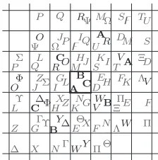
As an example, consider the distinct difference configu-ration given at the start of this introduction. If we use this configuration for key distribution in Scheme 1, each node stores three keys. Figure 1 illustrates this key distribution: each square in the grid represents a node, and each symbol contained in a square represents a key possessed by that node. The central square stores keys marked by the letters A, B andC; two further nodes share each of these keys, which are marked in bold. Letters in standard type represent keys used to connect the central node to one of its neighbours via a two-hop path, other keys are marked in grey. Note that we have only illustrated some of the keys; the pattern of key sharing extends in a similar manner throughout the entire network. See [2] for a comparison of how Scheme 1 outperforms related key predistribution schemes in the literature.
Note that the sensors’ strictly limited battery power limits the range over which they can feasibly communicate. In support of Scheme 1, distinct difference configurations with bounds on the distance between any two dots in the configu-ration were considered in [2]. Supposing that each sensor has a fixed communication range r, a DD(m, r) is defined to be a DD(m) in which the Euclidean distance between any two points of the configuration is at most r. From an application point of view, it is only necessary for a pair of nodes to share a key if they are located within communication range of each
[image:4.612.378.490.41.154.2]A A A B B B C C C D D D E E E F F F G G G H H H I I I J J J K K K L L L M M M N N N O O O P P P Q Q Q R R R S S S T T U U V V V W W W X X X Y Y Z Z Z ∆ ∆ ∆ Φ Φ Γ Γ Θ Θ Λ Λ Ξ ΞΠ Π Π Σ Σ Υ Υ Ψ Ψ Ω Ω ̥ ̥
Fig. 1. Key distribution using a distinct difference configuration.
other; the use of aDD(m, r)in Scheme 1 ensures that this is the case.
While Scheme 1 was designed to suit wireless sensor networks in which the sensors are arranged in a square grid, for certain applications a hexagonal arrangement of sensor nodes may be preferred, as it yields the most efficient packing of sensors (see [11] for details of circle packings in the plane). Section II defines the hexagonal model more precisely and discusses the relationship between the two models. Scheme 1 is easily adapted to suit sensors arranged in a hexagonal grid by replacing theDD(m)by aDD∗(m), which we informally define to be a set ofmdots on a hexagonal grid such that the vector differences between pairs of dots are distinct. We define aDD∗(m, r)to be aDD∗(m)in which the Euclidean distance between any pair of dots is at mostr. Another model that is natural when working with either the square or hexagonal grids is to replace the Euclidean metric by its discrete equivalent: the Manhattan metric (in the case of square grids), or an analogous metric on the hexagonal grid; in this case, we use the notation
DD(m, r) and DD∗(m, r), respectively. Constructions and bounds on the parameters for such configurations were studied in [1]. Section II contains a summary of the relationships between configurations based on different grids when using different metrics.
C. Contributions
Recall that wireless sensor networks rely on data being relayed via intermediate nodes using a series of hops. From an efficiency perspective it is thus of interest to consider properties relating to the nodes that can be reached from a specific node by means of a restricted number of hops.
If two nodesAandBare within communication range and share a key we say there is a one-hop path betweenAandB. If they do not share a key, however, they may still be able to establish a secure connection if there is a nodeCthat is within range ofAandB and shares a key with each of them. This is referred to as a two-hop path; more generally we considerk -hop paths of the formA−C1−C2. . .−Ck−1−B, where there
generally, we can define thek-hop coverage to be the expected
number of nodes with which a given node can communicate via some ℓ-hop path with1≤ℓ≤k (where we do not count the given node itself).
This measure is important from the point of view of our application, since it captures the ability of the network to transmit information in the context of the nodes’ limited capacity to relay messages. The case when k= 2 is the most studied situation in the literature, since results are often easier to establish than in the general k-hop case. Lee and Stinson use the notationPr1+Pr2to describe this quantity, referring
to it as the local connectivity [12]; similar metrics are used in [13], [14], and various related measures of the expected number of hops required for secure communication between two nodes are prevalent in the sensor network literature [7], [15], [16].
We define the k-hop coverage of a distinct difference con-figuration to be thek-hop coverage of the resulting instance of Scheme 1. In [2] a number of distinct difference configurations with good two-hop coverage were found by computer search. However no concrete construction techniques were provided. In this paper we provide an exposition of the two-hop coverage case, as well as consider the generalisation tok-hop coverage. Section III is devoted to a study of the k-hop coverage Ck(D)obtained by the use of the distinct difference configu-ration D ={v1,v2, . . . ,vm} in Scheme 1. Subsection III-A
shows how to calculate the k-hop coverage from the vectors
v1,v2, . . . ,vm. In Subsection III-B we study configurations
where Ck(D)is as large as possible, and show a connection
between such configurations andBhsequences (a well studied
concept in combinatorial number theory). We determine the maximum value of the k-hop coverageCk(D)whereD is a
DD(m)(or a DD∗(m)), and show thatD achieves this level ofk-hop coverage if and only ifD is a B2k sequence. If we
restrictDto be aDD(m, r)for some small integerr, we might no longer be able to achieve this maximum value ofCk(D): we provide bounds on the smallest value ofrfor which there exists a configuration D which is a DD(m, r) with Ck(D)
maximal. We also provide similar bounds on this smallest value of r when we consider configurations DD∗(m, r) in the hexagonal grid. Finally, in Subsection III-C, we provide a lower bound on Ck(D) and characterise those configurations
that meet this lower bound.
Using a distinct difference configuration with maximal k-hop coverage ensures that as many users as possible are connected by k-hop paths. However, in many applications these paths are used to establish keys which are later used for direct communication between the two end nodes: thus we are only interested in k-hop paths whose start and end nodes are within communication range. For these applications, rather than optimising the total number of pairs of users connected by k-hop paths we wish to optimise coverage in a locally defined region: We say that a DD(m)orDD∗(m)achieves complete k-hop coverage with respect to a regionR and pointp∈R if every point inRcan be reached by a two-hop path fromp. This means that every nodeu can communicate via ak-hop path with the nodes in the region corresponding to a shift ofR that movesptou, giving Scheme 1 good local connectivity. In
0 56 12
4 3 √
3 1 √
2
√
2 −−−→ξ 5 0 2
6
4 1
[image:5.612.352.522.63.133.2]3
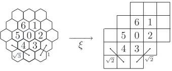
Fig. 2. A transformation from a hexagonal grid to a square grid (grid points are represented by the centres of the cells).
Section IV we give a construction for aDD(m)that achieves complete two-hop coverage with respect to the centre of a
(2p−3)×(2p−1)rectangle when pis prime.
II. DIFFERENTGRIDS ANDDIFFERENTMETRICS
A. Square and Hexagonal Grids
Suppose that the sensor nodes are arranged in a square grid, and the shortest distance between a pair of nodes is1. So we tile the plane by unit squares, and think of the nodes as lying at the centres of these squares. By supposing one of the nodes is at the origin, the location of a node can be identified with a vector inZ2. Because of this, we callZ2 the square grid.
A hexagonal arrangement of sensor nodes is obtained by tiling the plane with regular hexagons and placing a node at the centre of each hexagon. We suppose that one of the nodes is located at the origin and the shortest distance between two nodes is 1. In a similar way to the square grid, the locations of the nodes can be represented by vectors in the set ΛH = {λ(1,0) +µ(−1/2,√3/2)|λ, µ ∈ Z}, which we call the hexagonal grid.
We have already defined a (square) distinct difference configurationDD(m)to be a setD={v1,v2, . . . ,vm} ⊆Z2
ofmdots with the property that the difference vectorsvi−vj
fori 6=j between any pair of dots are distinct. In the same way, we define a (hexagonal) distinct difference configuration
DD∗(m)to be a setD={v1,v2, . . . ,vm} ⊆ΛH ofm dots
in the hexagonal grid with the property that the difference vectors vi−vj for i 6= j are distinct. A hexagonal distinct
difference configuration can be used in Scheme 1 for sensors arranged in a hexagonal grid, provided that shiftsu∈ΛH are used: as in the square grid, every node is assignedmkeys and the distinct difference property implies that any pair of nodes has at most one key in common. We define aDD∗(m, r)to be aDD∗(m)in which the Euclidean distance between any pair of dots in the configuration is at mostr: these configurations must be used when the wireless communication range of a sensor node isr.
The mapξ:R2→R2 defined by
ξ: (x, y)7→(x+√y
3, 2y
√
3)
(a) Lee sphere of radius 2 (b) Hexagonal ball of radius 1
Theorem 1. If D = {v1,v2, . . . ,vm} is a DD∗(m), then
ξ(D) = {ξ(v1), ξ(v2), . . . , ξ(vm)}is aDD(m). Similarly, if
D′is aDD(m), thenξ−1(D′)is aDD∗(m).
Proof: Sinceξis a linear bijection, we have thatvi−vj= vk −vℓ if and only if ξ(vi)−ξ(vj) = ξ(vk)−ξ(vℓ); the
first statement of the theorem follows directly. The second statement follows asξ−1 is also a linear bijection.
Despite Theorem 1, the square and hexagonal models differ once we are interested in distances between dots, sinceξdoes not preserve Euclidean distances. Fig. 2 shows a line segment of length √3that transforms into one of length√2, and one of length 1 that also transforms into one of length√2. It is straightforward to show that these line segments represent the maximum extent to whichξcan extend or contract the length of a vector; we formalise this in the following theorem:
Theorem 2.IfDis aDD∗(m, r)thenξ(D)is aDD(m, r√2). IfD′is aDD(m, r), thenξ−1(D′)is aDD∗(m, rp
3/2).
Thus we can convert between results aboutDD(m, r)and re-sults aboutDD∗(m, r)(although the bounds on the converted lengths are not tight in general).
B. Alternative Metrics on Grids
In [2], the need to take sensor nodes’ communication range into account when using distinct difference configurations to distribute keys to sensors arranged in a square grid motivated the definition of a DD(m, r) based on a Euclidean measure of distance. However, when working with a square grid it is natural to consider the Manhattan metric (also known as the Lee metric), in which the distance between dots with coordinates(i1, j1)and(i2, j2)is given by|i1−i2|+|j1−j2|.
Distinct difference configurations DD(m, r) in which the distance between dots in the configuration is at most rin the Manhattan metric were studied in [1]. A ball of radiusrin this metric is referred to as a Lee sphere (Fig. 3a), and for small rgives a reasonable approximation of a Euclidean circle. The well-known relation between these two metrics is expressed in the following theorem, which permits conversion between results aboutDD(m, r) and results aboutDD(m, r).
Theorem 3. For r ∈ Z, a DD(m, r) is a DD(m, r) and a DD(m, r)is aDD(m,⌈√2r⌉).
For the hexagonal grid, we say that a given point is adjacent to the six grid points that lie at Euclidean distance 1 from that point (for example, in Fig. 2 the points at the centres of cells 1,2, . . . ,6 are adjacent to the point at the centre of cell 0). We can then define a graph in which the grid points correspond to vertices, with edges connecting vertices
whose grid points are adjacent. This gives rise to a hexagonal
metric in which the distance between two points is the length
of the shortest path between the corresponding vertices in the graph. A distinct difference configuration in which the hexagonal distance between any two points is at most r is denotedDD∗(m, r). The relation between the hexagonal and Euclidean metrics can be used to prove the following theorem:
Theorem 4.Forr ∈ Z, a DD∗(m, r)is a DD∗(m, r) and a DD∗(m, r)is aDD∗(m,⌈√2
3r⌉).
We note that the hexagonal metric gives a closer approxima-tion to the Euclidean distance than the Manhattan metric.
III. k-HOPCOVERAGE
In this section we investigate the properties of distinct difference configurations with respect to theirk-hop coverage. While the motivation for this work comes from the application, the results are of independent combinatorial interest.
A. Characterisingk-hop coverage
LetDbe a (square or hexagonal) distinct difference config-uration given byD={v1,v2, . . . ,vm}. DefineCk(D)to be
the number of non-zero vectors that can be written as the sum ofkor fewer difference vectors. So Ck(D)is the number of
non-zero vectors of the form
ℓ X
i=1
(vαi−vβi) (1)
where αi, βi ∈ {1,2, . . . , m} with αi 6= βi and where 0 ≤
ℓ≤k.
Theorem 5.Suppose thatDis used in Scheme1. Then thek -hop coverage of the scheme is equal toCk(D).
Proof: Let x be any fixed node. Two nodes that share a key are located at points of the form vi+u and vj+u
for somei, j∈ {1,2, . . . , m} and some shiftu. This implies that the vector difference between their positions is vi−vj,
which is a difference vector of D. Hence a one-hop path between nodes with keys distributed according to Scheme 1 corresponds to a difference vector of the underlying distinct difference configuration. So there is an ℓ-hop path fromx to another node y if and only if the vector difference between their positions is the sum of ℓ difference vectors. Note also thatx=yif and only if this sum is the zero vector: since we do not countxin thek-hop coverage, we are only interested in sums of the form (1) which are non-zero. So Ck(D)is equal
to thek-hop coverage of Scheme 1 implemented using D, as required.
Proof: Theorem 5 shows that we must show that
Ck(D) = Ck(D′). But Ck(D) and Ck(D′) both count the
number of non-zero vectors that can be expressed as the sum of k or fewer difference vectors (of D or D′ respectively). The theorem now follows, since ξ is a linear bijection.
B. Maximalk-hop coverage
In this subsection we determine the maximalk-hop coverage of a DD(m). By Theorem 6, these results apply equally to a DD∗(m). We begin with some preliminary notation and lemmas.
For a non-negative integerkwe define a setHk ofm-tuples
of integers as follows:
Hk= (
(a1, a2, . . . , am)∈Zm
m X i=1
ai= 0, X
{i:ai>0}
ai=k )
.
For example, when m = 3 the triple (0,0,0) is the unique element of H0, the triple (1,−1,0) is a typical element of
H1, and the triples(2,−2,0),(2,−1,−1)and(1,1,−2) are
typical elements of H2. The following results about the sets
Hk are easily proved.
Lemma 7.Define the setsHk as above.
(i) Leta∈Hk1 andb∈Hk2. Thena+b∈Hk3 wherek3
is an integer satisfying0 ≤ k3 ≤k1+k2. In particular,
if a non-zerom-tuplevis a sum ofk m-tuples fromH1,
thenv∈Hk3 for somek3satisfying1≤k3≤k.
(ii) Leta∈Hk1andb∈Hk2witha6=b. Thena−b∈Hk3
wherek3is an integer satisfying1≤k3≤k1+k2.
(iii) Any element ofHk1 may be written as the sum of k1
elements fromH1.
The connection between Hk and the k-hop coverage of DD(m)is given by the following theorem:
Theorem 8. The k-hop coverage of a DD(m) is at most Pk
i=1|Hi|, with equality if and only if all the vectors Pm
i=1aiviwith(a1, a2, . . . , am)∈Skj=0Hjare distinct.
Proof: The difference vectors of D are precisely the vectors of the formPm
i=1aiviwherea∈H1. By Lemma 7 (i)
and (iii), a vector is a sum of k or fewer difference vectors if and only if it can be written in the form Pm
i=1aivi
with (a1, a2, . . . , am) ∈ Skj=0Hj. The zero vector can
al-ways be written in this form, since the sum is zero when
(a1, a2, . . . , am) ∈ H0. Since and we are only interested in
non-zero vectors, we find that
Ck(D) + 1 = m X i=1
aivi wherea∈ k [ j=0 Hj ≤ k X i=0
|Hi| !
= 1 + k X
i=1
|Hi| !
[image:7.612.319.552.79.145.2],
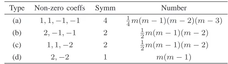
TABLE I COUNTING ELEMENTS INH2
Type Non-zero coeffs Symm Number
(a) 1,1,−1,−1 4 1
4m(m−1)(m−2)(m−3)
(b) 2,−1,−1 2 1
2m(m−1)(m−2)
(c) 1,1,−2 2 1
2m(m−1)(m−2)
(d) 2,−2 1 m(m−1)
and it is clear that equality is satisfied if and only if the vectors Pm
i=1aivi wherea∈
Sk
j=0Hjare distinct. Thus the theorem
follows.
Corollary 9.The two-hop coverage of aDD(m)is at most 1
4m(m−1)(m−2)(m−3) +m(m−1)(m−2) + 2m(m−1) = 1
4m(m−1)(m
2
−m+ 6).
Proof: By Theorem 8 the two-hop coverage is at most |H1|+|H2|. It is clear that|H1|=m(m−1), since the
m-tuples inH1have exactly two non-zero components, one equal
to1 and one equal to−1. To determine|H2|, note that there
are four types of element in H2, corresponding to the four
possibilities for the multiset of non-zero coefficients in an m-tuplea∈H2(see Table I). The number of elements inH2of
each type is equal to(1/s)m!/(m−t)!, wheretis the number of non-zero components in an m-tuple of this type, and s is the number of symmetries that preserve such m-tuples. Thus
|H2| = 14m(m−1)(m−2)(m−3) +m(m−1)(m−2) +
m(m−1), and so the bound of the corollary follows. In order to show that the bound of Theorem 8 and Corol-lary 9 is tight, we must show that there exists aDD(m)given by D={v1,v2, . . . ,vm} such that the vectors Pmi=1aivi,
wherea ∈ H0∪H1∪ · · · ∪Hk, are all distinct. This is not
difficult to do: for example we may choosevi= ((2k+1)i,0)
fori= 1,2, . . . , m. We say that a configuration meeting the bound of Theorem 8 has maximalk-hop coverage. Note that
the example we have just given of a configuration with max-imalk-hop coverage is not useful for our application, as the dots in the configuration are exponentially far apart: we would like to construct aDD(m, r)withrsmall having maximal k-hop coverage. In order to do this, we now aim to characterise those configurations with maximalk-hop coverage in terms of the much studied concept ofBhsequences (see below). First,
we make the following observation.
Lemma 10. Thek-hop coverage of aDD(m)given byD =
{v1,v2, . . . ,vm}meets the bound of Theorem8if and only if Pm
i=1civi6= 0for allc∈S2i=1k Hi.
Proof: Suppose thatDdoes not meet the bound of Theo-rem 8. Then TheoTheo-rem 8 implies thatPm
i=1aivi=Pmi=1bivi,
where a,b ∈ Sk
i=0Hi and a 6= b. Writing c = a−b we
have thatPm
i=1civi= 0, andc∈
S2k
i=1Hi by Lemma 7 (ii)
above.
Conversely, suppose that there existsℓ∈ {1,2, . . . ,2k}and
writecas the sum ofℓdifference vectors. Since multiplying a difference vector by the scalar−1produces another difference vector, we may write c = a−b, where a,b are the sum of⌊ℓ/2⌋and⌈ℓ/2⌉difference vectors respectively. Note that
a 6=bsince c6= 0. But a∈H⌊ℓ/2⌋ and b∈H⌈ℓ/2⌉, where
0≤ ⌊ℓ/2⌋ ≤ ⌈ℓ/2⌉ ≤ ⌈2k/2⌉=k, and so Theorem 8 implies thatD does not meet the bound, as required.
Definition 1. Let A be an abelian group. Let D =
{v1,v2, . . . ,vm} ⊆ Abe a sequence of elements of A. We say thatDis aBh sequence over Aif all the sums
vi1+vi2+· · ·+vih with1≤i1≤ · · · ≤ih≤m (2)
are distinct.
Bh sequences (sometimes known as Bh-sets) have been
studied for many years, mainly in the case where A = Z. See Graham [17], Halberstam and Roth [18], Lindstr¨om [19], O’Bryant [20], for example.
Example 1.Letq be a prime power, lethbe an integer such thath≥ 2and letαbe a primitive element ofGF(qh). Bose and Chowla [21] have shown that the set{a∈Zqh−1|αa−α∈
GF(q)}is aBhset inZqh−1containingqelements.
The following theorem demonstrates the relation betweenBh
sequences and distinct difference configurations.
Theorem 11.Letkbe a fixed integer, wherek ≥2. LetD =
{v1,v2, . . . ,vm} ⊆ Z2. ThenD is aDD(m)with maximal
k-hop coverage if and only ifDis aB2ksequence overZ2.
Proof: Suppose D is a B2k sequence over Z2. We aim
to show thatD is aDD(m)with maximal k-hop coverage. Ifvi =vj fori6=jthen(2k−1)v1+vi= (2k−1)v1+vj
and soDcannot be aB2ksequence. This contradiction implies
that the vectors are all distinct.
Suppose that vi−vj = vi′ −vj′, wherei 6=j, i′ 6= j′. Then (2k−2)v1+vi+vj′ = (2k−2)v1+vi′+vj. This
contradicts the fact thatDis aB2k sequence, unlessi=i′and
j′ = j. Thus D has the distinct differences property. Hence D is aDD(m).
Suppose, for a contradiction, that D does not have
max-imal k-hop coverage. By Lemma 10 there exists a =
(a1, a2, . . . , am)∈H1∪ · · · ∪H2k such thatPmi=1aivi= 0.
Definebby
bi=
ai when ai≥0 0 otherwise.
Definecby the equationa=b−c. Then the components ofb
andcare all non-negative. Writingt=Pm
i=1bi=Pmi=1ci= P
ai>0ai, the definition ofH1, H2, . . . , H2k implies that1≤
t≤2k. Sincea is non-zero,b6=c. But then our choice ofa
implies that
(2k−t)v1+
m X
i=1
bivi= (2k−t)v1+
m X
i=1
civi.
There are exactly2ksummands on both sides of this equality, soDcannot be aB2k sequence. This contradiction shows that
D has maximalk-hop coverage, as required.
Now suppose that D is a DD(m) with maximal k-hop coverage. Assume thatDis not aB2ksequence, so there exist
two distinct sums of the form (2) that are equal. By cancelling terms that occur in both sums, we find that Pm
i=1bivi = Pm
i=1civi, where the coefficients bi, ci are all non-negative
and where Pm
i=1bi = Pmi=1ci = t for some integert such
that 1 ≤ t ≤ 2k. But defining ai = bi−ci we find that (a1, a2, . . . , am) ∈ Ht and Pmi=1aivi = 0. Hence D does
not have maximalk-hop coverage, by Lemma 10, as required.
The following construction converts a known construction for aB2k sequence inZq2k−1 into a B2k sequence inZ2, which
is aDD(m)with maximalk-hop coverage by Theorem 11.
Construction 1 Letkbe a fixed integer such thatk ≥ 2. Let qbe a prime power, and letq2k
−1 = abwhereaandbare coprime. Then there exists a setX ⊆Z2of dots that is doubly periodic with periodsaandb, and such that the intersection of X with anyb×arectangle is aDD(q)with maximal k-hop coverage.
Proof: The construction of Bose and Chowla [21]
de-scribed in Example 1 shows there is a B2k sequence over
Zq2k−1 consisting of q elements. Note that by the Chinese
Remainder Theorem there is a group isomorphismZq2k−1→
Za×Zb given byx7→ (xmoda, xmodb). Thus there are
elementsv1,v2, . . . ,vq ∈Za×Zb that form aB2k sequence
over Za×Zb. Let ρ:Z2 →Za×Zb be the map defined by
ρ((x, y)) = (xmoda, ymodb). We defineX ⊆Z2to be the set of vectorsv∈Z2 such thatρ(v)∈ {v1,v2, . . . ,vq}.
Sinceρ((x, y)) =ρ((x+ia, y+jb))for anyi, j∈Z, we see thatX is doubly periodic with periodsa and b respectively. LetR be anb×arectangle inZ2. For alli∈ {1,2, . . . , m}, there is a unique vi ∈ R such that ρ(vi) =vi. Hence X ∩
R = {v1,v2, . . .vq}. Moreover, v1,v2, . . . ,vq form a B2k
sequence overZ2, since if there are two sums of the form (2) that are equal, then the images of these sums underρare also equal, which contradicts the fact that v1,v2, . . . ,vq form a
B2ksequence overZa×Zb. Thusv1,v2, . . . ,vqform aDD(q)
with maximalk-hop coverage by Theorem 11, as required. This construction can be used to prove the existence of a
DD(m, r) with maximalk-hop coverage wherer is small:
Theorem 12.Letkbe a fixed integer such thatk ≥2. Define c = (π/16)21/k. Then there exists aDD(m, r)with maximal
k-hop coverage such thatm∼cr1/k.
Proof: LetS ⊆Z2 be the set of points inZ2 contained in a circle of radius⌊r/2⌋about the origin. Note that |S| = (π/4)r2+O(r) (by the Gauss Circle Problem).
Let qbe the smallest prime power such that qk >2r. We
have thatq≤(2r)1/k+((2r)1/k)5/8wheneverris sufficiently
large by a classical result of Ingham [22] on the gaps between primes. In particular,q∼(2r)1/k.
Define the integeraby
a=
qk
−1 whenq is even,
(qk
−1)/2 whenqk
≡3 mod 4,
(qk+ 1)/2 whenqk
Defineb= (q2k
−1)/a. Sincegcd(qk
−1, qk+ 1) = 1 when
q is even andgcd(qk
−1, qk+ 1) = 2whenqis odd, we find
that a and b are coprime. Moreover, our choice of q shows that r ≤ a ≤ b. Let X be the set of dots in Z2 given in Construction 1.
The average number of dots in a shift of S by an element of Z2 is |S|q/(ab), and so we can find a shift T of S such that |T ∩X| ≥ |S|q/(ab). Define D ⊆ T ∩ X to be a subset of size m, where m = ⌈|S|q/(ab)⌉. Note that m∼(π/4)r2q/(2r)2
∼(π/16)21/kr1/k. Since T is a sphere
of radius⌊r/2⌋, any pair of dots inDare at distance at mostr. Moreover, the fact thatr≤a≤b implies thatT is contained in ab×arectangleR. By Construction 1,R∩X is aDD(q)
with maximal k-hop coverage. Since D ⊆T∩X ⊆R∩S, we see that D is a DD(m, r) with maximalk-hop coverage. So the theorem follows, as required.
Combining Theorems 2, 6 and 12, we have the analogous result for the hexagonal grid:
Corollary 13.Letkbe a fixed integer such thatk≥2. Define c′ = (π/16)21/k 2
3
1/2k
. Then there exists aDD∗(m, r)with maximalk-hop coverage such thatm∼c′r1/k.
For any fixed values of m and k, we define r(k, m) to be the smallest value of rsuch that there exists a DD(m, r)
with maximal k-hop coverage. It is an important problem to determine r(k, m). The construction in Theorem 12 provides an upper bound on r(k, m), showing that when k is fixed and m→ ∞ we haver(k, m) =O(mk). We now provide a
corresponding lower bound onr(k, m), which shows that the construction in Theorem 12 is reasonable:
Theorem 14. Let k be an integer such that k ≥ 2. Then mk
√
πk!·k +o(m k)
≤r(k, m)≤1 2
16
π k
mk+o(mk).
Proof: The upper bound is proved in Theorem 12.
To prove the lower bound, let D be a DD(m, r) with maximalk-hop coverage, wherer=r(k, m). The definition of maximalk-hop coverage and Theorem 5 show thatCk(D) = Pk
i=1|Hi|. Let B ={(a1, a2, . . . , am) ∈Hk : |{i : ai 6= 0}|= 2k}. Clearly|B|= m!
(m−2k)!k!2 and
k X
i=1
|Hi|= m!
(m−2k)!k!2 +o(m
2k) =m2k
k!2 +o(m 2k).
SoCk(D) = mk!22k +o(m2k).
Every vector counted by Ck(D) is the sum of at most k difference vectors ofD. Each difference vector has length at most r, and so every vector counted by Ck(D) is contained
in a circle of radius kr centred at the origin. Such a circle contains at most π(kr)2+O(r) vectors in Z2 (by Gauss’s
solution to the Gauss circle problem). Thus
m2k
k!2 +o(m
2k) =Ck(D)
≤π(kr)2+O(r),
which implies the lower bound of the theorem, as required. For the hexagonal grid, we denote the smallest r for which there exists a DD∗(m, r) with complete k-hop coverage by
r∗(m, k). Combining Theorems 14 and 2, we have the fol-lowing.
Theorem 15.Ifk≥2then q
3 2
mk
√πk!
·k+o(m k)
≤r∗(k, m)≤ q
3 2 1 2
16
π k
mk+o(mk).
In the casek= 1, we can use the results of [1] to give tighter bounds, as every distinct difference configuration has a one-hop coverage ofm(m−1), which is thus maximal.
Theorem 16.We have that 2
√πm+o(m)≤r(1, m)≤ 2
µm+o(m),
whereµ≈0.914769is the maximum value of((π/2)−2θ+ sin 2θ)/cosθon the interval0≤θ≤π/4.
Proof: It is proved in [1] that if a DD(m, r) exists, then m ≤ √2πr+O(r2/3), which gives rise to the lower
bound on r(1, m). Furthermore, [1] contains a construction of aDD(m, r)withm= (µ/2)r+o(r)dots, from which we derive the upper bound.
The paper [1] also contains analogous results in the hexagonal grid. From these, we can deduce the following bounds on r∗(1, m):
Theorem 17.We have that
√
2 31/4
√π m+o(m)≤r∗(1, m)≤21/231/4
µ m+o(m), whereµis defined as in Theorem16.
Recall that we introduced the Manhattan and hexagonal metrics on the square and hexagonal grids respectively in Section II. We conclude this subsection with a brief discussion about the situation when we use these metrics rather than Euclidean distance. For integersk andm, definer(k, m) to be the smallest integer r such that there exists a DD(m, r)
with maximalk-hop coverage, and definer∗(k, m) to be the smallest integer r such that there exists a DD∗(m, r) with maximalk-hop coverage.
Theorem 18. Let k be a fixed integer, k ≥ 2. There exist constants c1, c2, c3 andc4 such that for all sufficiently large
integersm
c1mk≤r(k, m)≤c2mkand
c3mk≤r∗(k, m)≤c4mk.
Proof: By Theorem 3, a DD(m, r)with maximal k-hop coverage is also a DD(m, r) with maximal k-hop coverage. Sor(k, m)≤r(k, m). Moreover, a DD(m, r) with maximal k-hop coverage is a DD(m,⌈√2r⌉) with maximal k-hop coverage, so r(k, m)≤ ⌈√2r(k, m)⌉. The first statement of the theorem now follows by Theorem 14.
The proof of the second statement of the theorem is similar, using Theorems 4 and 15 in place of Theorems 3 and 14 respectively.
Theorem 19.We have that
r(1, m) =√2m+o(m).
Moreover,
(2/√3)m+o(m)≤r∗(1, m)≤(2/µ)m+o(m),
whereµ= (2/3)3/2(1 + 2√7)/(p
2 +√7)≈1.58887.
C. Minimumk-hop coverage
Having established an upper bound for the k-hop coverage of aDD(m)(and hence of aDD∗(m)), we now consider the smallest values it can take.
Theorem 20. The k-hop coverage of a DD(m) is at least km(m−1).
Proof: The one-hop coverage of aDD(m)ism(m−1). ForD={v1,v2, . . . ,vm}aDD(m), letu= (d, e)be the
difference vector with|d|as large as possible. If there is more than one choice foru, chooseuwith|e| as large as possible subject to |d| being maximal. Without loss of generality, we can assume thatd >0ande≥0(if not we can flip and rotate the array to obtain an equivalent array with such vector).
LetS1 be the set ofm(m−1)vectors that can be reached
by one-hop paths from the origin. ThenS1 can be written as
the disjoint union of the two sets
S1+={(x, y)|(x, y)∈S1, x >0 or(x= 0andy >0)}
andS1− ={−(x, y)|(x, y)∈S1+}. Fori >1, we define
Si={w+ (i−1)u|w∈S1+} ∪
{(−w−(i−1)u|w∈S1+}.
Asuis a difference vector ofD, the vectors ofSi can all be
reached byi-hop paths from the origin. Furthermore,Si∩Sj=
∅fori6=jand|Si|=m(m−1). Hence, the theorem is proved.
For certain values of m there existDD(m) for which the above bound is tight. For example, consider the following
DD(3):
• • •
The difference vectors in this example are
{±(1,0),±(2,0),±(3,0)}, and hence any of the 6k vectors of the form±(t,0)for0< t≤3kcan be reached by ak-hop path.
We can construct more examples where the bound is tight as follows. A Golomb ruler is a set M of m integers such that the differencesx−y wherex, y∈M andx6=y are all distinct. A Golomb ruler is perfect if
{u−v:u, v∈S}={i∈Z:|i| ≤m(m−1)/2}. For example, the sequence {0,1,3} is a perfect Golomb ruler. The DD(3) above was constructed from this sequence by taking appropriate multiples of the vector (1,0). More generally, ifM is a perfect Golomb ruler then a configuration D consisting of the vectors r+iswherei∈M is aDD(m)
with ak-hop coverage ofkm(m−1), and so meets the bound
of Theorem 20. We say that D is equivalent to a perfect
Golomb ruler if we can construct it in this way. In fact, we
will now show that aDD(m)meets the bound of Theorem 20 if and only if it is equivalent to a perfect Golomb ruler.
Lemma 21.Letkbe an integer,k≥2. SupposeDis aDD(m) in which there are differencesdandd′ that are not parallel. Then thek-hop coverage ofDis strictly greater thankm(m−
1).
Proof: Define the difference vectoruand the sets Si as
in the proof of Theorem 20. The set of difference vectors not parallel touis non-empty by assumption. Letvbe a difference vector whose projection in the direction perpendicular to u
has lengthp(v)as large as possible. Since k≥2, thek-hop coverage ofD is at least
|S1∪S2∪ · · · ∪Sk∪ {2v}|.
The argument in Theorem 20 shows the sets Si are disjoint
and have orderm(m−1). So the theorem follows if we can show that2v6∈S1∪S2∪ · · · ∪Sk. But any vector inSi can
be written in the formw±(i−1)uwherew is a difference vector, and therefore
p(w±(i−1)u) =p(w)≤p(v)<2p(v) =p(2v).
Hence2vdoes not lie in any of the sets Si, as required.
Theorem 22.Letkbe an integer such thatk≥2, and letDbe aDD(m). ThenDmeets the bound of Theorem20if and only if it is equivalent to a perfect Golomb ruler.
Proof: It is easy to see that ifDis equivalent to a perfect Golomb ruler, thenD meets the bound of Theorem 20.
Let D be a DD(m)that meets the bound of Theorem 20. The set Sℓ defined in the proof of Theorem 20 is a set of
m(m−1) vectors that can be reached by anℓ-hop path from the origin, but cannot be reached by a path of length ℓ−1. ThusCk(D)≥C2(D) + (k−2)m(m−1), soD meets the
bound of Theorem 20 in the case k = 2. So to prove the theorem, we need only consider the casek= 2.
Let r be a vector in D. Lemma 21 implies that all the difference vectors inD are parallel to a fixed vectoru. Lets
be the shortest vector inZ2 that is parallel tou. Then (since
Z2is a lattice)D⊆ {r+is|i∈Z}. ThusD is equivalent to a Golomb ruler M ⊆Z. Without loss of generality, we may assume that the greatest common divisor of the elements of M is1, for if the greatest common divisor is athen we can replacesbyasandM by(1/a)M.
It remains to show that M is perfect. The set S = {x− y|x, y ∈M} contains m(m−1) + 1 elements, since M is a Golomb ruler. A square reachable from the origin by a one-hop or two-hop path corresponds to an element ofS+S={a+
progression. Since S=−S and the greatest common divisor of the elements of M is1 we find thatS ={x∈Z| |x| ≤ m(m−1)/2}. So M is a perfect Golomb ruler, as required.
IV. ADD(m)WITHCOMPLETETWO-HOPCOVERAGE IN
ARECTANGLE
In Section III we explored the range of values that the k-hop coverage of a distinct difference configuration can take. When choosing a distinct difference configuration for use in Scheme 1 it may seem desirable to select a configuration with maximal two-hop coverage. However, from Theorem 14 we see that aDD(m, r)with maximal two-hop coverage has “approximately”m2=r, which places too great a restriction
on the maximum number of keys that each node can store in the resulting scheme. From a practical perspective it thus may be desirable to focus on connectivity within a localised region. In this section we give a construction of a DD(m) that ensures a two-hop path between a given pointxand any other grid point within a(2p−3)×(2p−1)rectangle centred atx, wherepis any prime greater than or equal to five. This allows the region to be tailored to the requirements of a specific application environment.
Our construction can be thought of as being based on the periodicity properties of aB2sequence inZ(p2
−p)proposed by
Ruzsa in [23], or as a consequence of a periodic generalisation of the Welch construction of a Costas array [24]. In Sub-section IV-A we discuss some properties of a related doubly periodic array that we will exploit later. In Subsection IV-B we present the construction and demonstrate that it achieves complete two-hop coverage.
A. The Welch Periodic Array
Definition 2. (Welch Periodic Array)Letαbe a primitive root modulo a primep. We define theWelch periodic arrayto be the set
Rp={(i, j)∈Z2|αj≡imodp}.
This array is doubly periodic in the sense that ifRpcontains
a dot at position(i, j)then it also contains dots at all positions of the form (i+λp, j+µ(p−1)) whereλ, µ ∈Z. It has a distinct difference property “up to periodicity”: see the lemma below. We say that dotsAandA′at positions(i, j)and(i′, j′) are equivalent, and we write A ≡ A′, if i′ = i+λp and j′ =j+µ(p−1) for someλ, µ∈Z.
Lemma 23.Letdandebe integers such thatd6≡0 modpand e 6≡0 mod (p−1). Suppose thatRp contains dotsAandB at positions(i1, j1)and(i1+d, j1+e)respectively, and dots
A′andB′at positions(i2, j2)and(i2+d, j2+e)respectively. ThenA≡A′andB ≡B′.
Proof: By the definition ofRp we have
i1≡αj1 modp
i2≡αj2 modp
i1+d≡αj1+emodp
i2+d≡αj2+emodp.
Eliminatingi1,i2 andd from these equations we get
(αe−1)(αj1 −αj2)
≡0 modp.
Sincee6≡0 mod (p−1), this implies thatj1≡j2mod (p−1).
The first two equations above then imply thati1≡i2modp.
We note that in addition, if Rp contains dots at (i, j) and (i+d, j) then d≡ 0 modp and if it contains dots at (i, j)
and (i, j+e) then e ≡ 0 mod (p−1). Thus we see that a vector (d, e)can occur at most once as a difference between two of the dots ofRpthat lie within any particular(p−1)×p
rectangle.
B. Construction of theDD(m)
We now define aDD(m)by choosing a finite subset of the dots inRp, as follows.
Construction 2 Letpbe an odd prime. Let(i, j)∈Z2be such thatRphas dots at (i, j)and(i+ 1, j+ 1). Note that such a position(i, j)exists. To see this, letiandjbe integers such that
αj ≡i≡ 1
α−1 modp.
The right-hand side of this equality is well-defined and non-zero modulop, and so there is a suitable choice for i andj. ClearlyRp has a dot at the position(i, j). But there is also a dot at(i+ 1, j+ 1)since
αj+1≡ α
α−1 ≡
1
α−1+ 1≡i+ 1 modp.
Consider the(p−1)×prectangleSbounded by the positions (i, j),(i+p−1, j),(i, j+p−2)and(i+p−1, j+p−2). By construction,Rp hasp−1 dots inS. Due to its periodic nature,Rpalso has dots at positions(i, j+ (p−1)),(i+p, j) and(i+p+ 1, j+p). We construct a configurationBby adding these three dots to the set of dots inRp∩S.
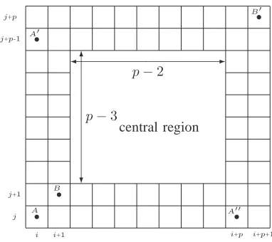
Our configurationB is shown in Fig. 3. The configuration is contained in a(p+ 1)×(p+ 2)rectangle. The border region of width2contains exactly5 dots:A, A′, A′′, BandB′. The
central region is a (p−3)×(p−2) rectangle. This region contains p−3 dots: one column is empty, but every other column and every row contains exactly one dot. Note that A≡A′≡A′′ andB ≡B′, but there are no other equivalent pairs of dots inB.
j+p j+p-1
j j+1
i i+1 i+p i+p+1
p−3
p−2
central region
A B A′
A′′
[image:12.612.80.271.52.222.2]B′
Fig. 3. The configuration B. The five dots shown are the dots that lie the border of width 2 of the(p+ 1)×(p+ 2) rectangle containing the configuration.
Proof: We have already remarked that B containsp+ 2
dots, all lying in a (p+ 1)×(p+ 2) rectangle. So it remains to show thatB satisfies the distinct differences property.
Suppose, for a contradiction, thatX andY, andX′andY′, are distinct pairs of dots in Bwith the same difference vector
(d, e).
Suppose that d∈ {0,−p, p} ore∈ {0,−(p−1),(p−1)}. A difference vector between a dot in the central region of our configuration and any other dot hasx−andy−coordinates of absolute value at mostp−1orp−2 respectively. Moreover, a central dot is the only dot in its row and column. So our assumption implies that none of X, X′, Y, Y′ can lie in the central region of our configuration. But the5×4ordered pairs of dots in the border region all have distinct difference vectors, and so we have a contradiction in this case.
So we may assume that d6∈ {0,−p, p} ande6∈ {0,−(p−
1),(p−1)}. In particular, since all dots lie in a(p+1)×(p+2)
rectangle, we see that d6≡0 modp ande6≡0 mod (p−1). Lemma 23 now implies that X ≡ X′ andY ≡ Y. If X = X′ then Y = Y′ which contradicts the fact that our pairs of dots are distinct. Hence X 6=X′. The fact that X ≡X′ now implies that X and X′ must lie in the border of our configuration. A similar argument implies the same is true for Y and Y′. As in the paragraph above, we now have a contradiction. Thus the lemma follows.
Our aim is to show (Theorem 27) thatBachieves complete two-hop coverage on a (2p−3)×(2p−1) rectangle relative to the central point of the rectangle. In order to demonstrate this, it is necessary to show that every vector(d, e)with|d| ≤ p−1 and|e| ≤p−2 can be expressed as a two-hop path of difference vectors from B. The following lemma proves this for the majority of such vectors(d, e).
Lemma 25.Any vector of the form(d, e), where dandeare non-zero integers satisfying|d| ≤p−1and|e| ≤p−2, can be expressed as the sum of two difference vectors fromB.
Proof: Consider the (p−1)×prectangle S defined in Construction 2, and letAbe the restriction ofRp to the(2p−
2)×2psubarray whose lower leftmost corner coincides with that ofS.
We partitionAinto four(p−1)×psubarrays as follows:
D3 D4
D1 D2
The periodicity of Rp means that the set of dots of Rp
contained in each subarray is a translation of the set of dots ofRp contained inD1. Moreover, sinceD1=S, all the dots
inD1 are contained in B.
We claim that each of the vectors(d, e)appears as the dif-ference of two points inA. Since the negative of a difference vector is always a difference vector, we may assume without loss of generality that d >0. Suppose thate >0. There is a unique position(i′, j′)∈ D1 such that
αj′ ≡i′≡ d
αe−1 modp.
It is easy to check, just as in Construction 2, thatRphas dots
at(i′, j′)and(i′+d, j′+e). Sincedandeare both positive,
(i′+d, j′+e)lies inA, and so our claim follows in this case. The argument for the case when e < 0 is exactly the same, except now we choose(i′, j′)∈ D
3. So the claim follows.
To prove the lemma, we need to show that each difference vector (d, e) can be written as the sum of two difference vectors ofB. This follows from the paragraph above and the following observations:
• Any vector connecting two dots of D1 is a difference
vector ofBby construction.
• Due to the periodicity ofRp, a vector connecting a dot
in D1 with a dot in D3 (or, similarly, a dot in D2 with
a dot in D4) can be expressed as the sum of the vector
(0, p−1)(which occurs as a difference between the dots AandA′ inB) and some other difference vector ofB. • A vector connecting a dot in D1 with a dot in D2 (or,
similarly, a dot inD3with a dot inD4) can be expressed
as the sum of the difference vector(p,0) (which occurs betweenAandA′′) and some other difference vector of
B.
• A vector connecting a dot in D1 with a dot in D4 is
the sum of the difference vector(p, p−1)(which occurs betweenB andB′) and some other difference vector of
B.
• A vector connecting a dot in D3 with a dot in D2 is the
sum of the difference vector(p,−(p−1))(which occurs betweenA′ andA′′) and some other difference vector of
B.
It remains to consider vectors that have a zero co-ordinate. We will use the following lemma in our proof that such vectors all occur as the sum of two difference vectors fromB.
Lemma 26.Lettbe a positive integer witht ≥3. LetFbe a set of integers satisfying the following properties:
(a) |F|=t+ 1,
(b) F ⊂ {−(t−1),−(t−2), . . . ,−1} ∪ {1,2, . . . , t−1} ∪ {t+ 1},
(d) ∃i∈ F \ {1,−(t−1), t+ 1}withi <0,
(e) ifi >0andi∈ F \ {1,−(t−1), t+ 1}theni−t /∈ F. Then each positive integer γ with 1 ≤ γ ≤ t −1 has a representation of the formγ=j−iwherei, j∈ F.
Proof: SinceF \ {1,−(t−1), t+ 1} containst−2 ele-ments, (e) implies thatF must contain precisely one element of each pair {i, i−t} fori= 2,3, . . . , t−1. Suppose, for a contradiction, that there exists a positive integerγ≤t−1that cannot be expressed as the difference between two elements ofF.
Suppose that γ > 1. Since 1, t+ 1 ∈ F, our assumption implies that 1−γ /∈ F and t+ 1−γ /∈ F. But 1−γ = (t+ 1−γ)−t, hence one of these numbers must be contained inF, which gives a contradiction in this case.
Suppose that γ = 1. The assumption implies thatF does not contain a pair of integers that differ by 1. If t is odd this implies that F \ {t+ 1} contains at most (t−1)/2 positive integers, and at most (t−1)/2 negative integers, hence F contains at most (t−1) + 1 = t integers, which contradicts (a). If t is even, then in order for the size of F to be t+ 1,
F \ {t+ 1} must contain t/2 positive integers, all of which are odd, and t/2 negative integers that are also all odd. This implies that for each positive odd integer 1< i < twe have thati∈ Fandi−t∈ F, which contradicts (e). So the lemma follows.
We can now combine these two lemmas to obtain our desired result:
Theorem 27.Letpbe a prime,p≥5. The distinct difference configuration B achieves complete two-hop coverage on a (2p−3)×(2p−1)rectangle relative to the central point of the rectangle.
Proof: By Lemma 25, any vector(d, e)from the centre of a(2p−3)×(2p−1)rectangle to another point of the rectangle can be expressed as the sum of two difference vectors ofBif dandeare non-zero.
We now consider vectors of the form (0, e)with0 < e≤ p−2. Such a vector can be expressed as the sum of two difference vectors ofBifBhas difference vectors of the form
(1, y′)and(1, y)withy′−y=e. The second coordinates of the set of difference vectors ofBof the form(1, y)withy6= 0
satisfy the conditions of Lemma 26 for t=p−1, since: (a) The left-most column of the array contains two dots; all
other columns contain a single dot apart from a single central column which is empty. So B has p difference vectors of the form(1, y)withy 6= 0.
(b) Except for the vector(1, p), all difference vectors ofBof the form(1, y)withy6= 0satisfy|y| ≤p−2.
(c) The vectors (1,1), (1,−(p−2)) and (1, p+ 1) are all difference vectors of B (as they occur as differences between dots in the border region of B, see Fig. 3). (d) The difference vectors of B of the form(1, y)cannot all
satisfy y > 0. This is obvious if the right-most central column contains a dot. If this column is empty and y is always positive, then the remaining(p−3)×(p−3)
central region must contain dots along a lower-left to top-right diagonal. Since p ≥ 5, two central dots have the
difference vector (1,1). Since dots A and B also have this difference vector, the distinct difference property is violated and so we have a contradiction, as required. (e) If (1, y) with y 6= 1, p is a difference vector of B then
(1, y−(p−1)) is not. For Lemma 23 implies that the dots involved must be equivalent, and so must be in the border region of our construction.
Lemma 26 now implies that any vector (0, e) with0 < e≤
p−2has an expression in the form(0, e) = (1, y′)+(−1,−y) where(1, y′)and (1, y) are difference vectors of B. Vectors of the form(0, e) with−(p−2)< e <0 can be written as
(1, y) + (−1,−y′).
In a similar manner, we can show that the first coordinates of the difference vectors of B of the form (x,1) satisfy the conditions of Lemma 26 witht=p, and hence any vector of the form (d,0) with 0 <|d| ≤ p−1 can be written as the sum of two difference vectors ofB. Thus the result is proved.
We can thus apply theDD(m)specified in Construction 2 to Scheme 1 in order to establish a key predistribution scheme which guarantees two-hop paths between a node and all of its neighbours within a surrounding rectangular region. This provides a powerful notion of local connectivity in order to facilitate connectivity across the wider network. The resulting scheme is also highly configurable, since the value ofp can be adjusted in order to tradeoff storage against the size of the fully connected local region.
V. CONCLUSION ANDOPENPROBLEMS
In this paper we have studied properties of distinct differ-ence configurations, which can be used to design efficient key predistribution schemes for wireless sensor networks based on grids.
In Section III we explored the k-hop coverage of a
DD(m, r). We characterised maximalk-hop coverage in terms ofB2k sequences overZ2, and we used a known construction
ofB2ksequences overZto produce aDD(m, r)with maximal
k-hop coverage and of the order ofr1/k dots. We provided an
argument that shows that the order of magnitude of the number of dots is correct (by bounding the functionsr(k, m)). These results indicate the range of achievable parameters, which in turn determine the connectivity properties of the resulting key predistribution schemes. It would be interesting to find better bounds on the leading coefficient of r(k, m), and it would be worthwhile determiningr(k, m)precisely for small values of k and m. Similar comments hold for the function r∗(k, m), and for the analogous situations using the Manhattan or hexagonal metric.
In Section IV we constructed aDD(m, r)with complete2 -hop coverage within a large rectangular region centred on the origin. This DD(m, r) can be used to design key predistri-bution schemes with excellent local connectivity properties. The area of the fully connected region is of the order of m2. It would be interesting to investigate whether there are
example a circle of large radius, would also be of practical interest. A further open problem is whether there exist any good constructions, for any natural region, achieving complete k-hop coverage fork≥3.
REFERENCES
[1] S.R. Blackburn, T. Etzion, K.M. Martin, and M.B. Paterson, “Two-dimensional patterns with distinct differences: Constructions, bounds and maximal anticodes,” preprint, 2008.
[2] S.R. Blackburn, T. Etzion, K.M. Martin, and M.B. Paterson, “Effi-cient key predistribution for grid-based wireless sensor networks,” in (R. Safavi-Naini, Ed) Proc. ICITS 2008, Lecture Notes in Computer Science 5155, Springer-Verlag, Berlin, pp. 54–69, 2008.
[3] K. R¨omer and F. Mattern. The design space of wireless sensor networks.
IEEE Wireless Communications Magazine, 11(6):54–61, 2004.
[4] S.A. C¸ amtepe and B. Yener, “Key Distribution Mechanisms for Wireless Sensor Networks: a Survey”, Rensselaer Polytechnic Institute Tech.
Re-port TR-05-07 March 2005.
[5] K.M. Martin and M.B. Paterson, “An Application-Oriented Framework for Wireless Sensor Network Key Establishment”, Electron. Notes Theor.
Comput. Sci., vol. 192, pp. 31–41, 2008.
[6] Y. Xiao, V.K. Rayi, B. Sun, X. Du, F. Hu and M. Galloway, “A survey of key management schemes in wireless sensor networks”, Comput.
Commun., vol. 30, pp. 2314–2341, 2007.
[7] L. Eschenauer and V.D. Gligor “A key-management scheme for dis-tributed sensor networks”, CCS ’02: Proc. of the 9th ACM Conference
on Computer and Communications Security, pp. 41–47, 2002.
[8] Institut f¨ur Chemie und Dynamik der Geosph¨are (ICG), Forschungszen-trum J ¨ulich: SoilNet – a Zigbee based soil moisture sensor network. http://www.fz-juelich.de/icg/icg-4/index.php?index=739, 2008. [9] Integrated smart sensing systems. http://dpi.projectforum.com/isss/11 ,
2007.
[10] J. McCulloch, P. McCarthy, S. M. Guru, W. Peng, D. Hugo, and A. Ter-horst. Wireless sensor network deployment for water use efficiency in irrigation. In REALWSN ’08: Proceedings of the Workshop on
Real-world Wireless Sensor Networks, pages 46–50, New York, NY, USA,
2008. ACM.
[11] J.H. Conway and N.J.A. Sloane, Sphere Packings, Lattices, and Groups, New York: Springer-Verlag, 1993.
[12] J. Lee and D.R. Stinson “On the construction of practical key predis-tribution schemes for distributed sensor networks using combinatorial designs”, ACM Trans. Inf. Syst. Secur., vol. 11(2), pp. 1–35, 2008. [13] W. Du, J. Ding, Y.S. Han, P.K. Varshney, J.Katz and A.Khalili “A
pairwise key pre-distribution scheme for wireless sensor networks”,
ACM Trans. Inf. Syst. Secur., vol. 8, pp. 228–258, 2005.
[14] H. Chan, A. Perrig and D. Song “Random key predistirbution schemes for sensor networks” IEEE Sumposium on Security and Privacy, pp. 197–213, 2003.
[15] S.A. C¸ amtepe, B. Yener and M. Yung “Expander graph based key distribution mechanisms in wireless sensor networks”, ICC ’06, IEEE
International Conference on Communications, pp. 2262–2267, 2006.
[16] D. Liu, P. Ning and R. Li ”Establishing pairwise keys in distributed sensor networks”, ACM Trans. Inf. Syst. Secur., vol. 8(1), pp. 41–77, 2005.
[17] S.W. Graham, “Bhsequences”, Analytic Number Theory, Vol. 1
(Aller-ton Park, IL, 1995), Birkhauser, Bos(Aller-ton, pp. 431–449, 1996.
[18] H. Halberstam and K.F. Roth, Sequences, Volume I, London: OUP, 1966. [19] B. Lindstr¨om, “OnB2sequences of vectors”, J Combinatorial Theory,
vol. 4, pp. 261–265, 1972.
[20] K. O’Bryant, “A complete annotated bibliography of work related to Sidon sequences”, Electron. J. Combin Dynamic Survey 11, 2004. [21] R.C. Bose and S. Chowla, “Theorems in the additive theory of numbers”,
Comment. Math. Helvet. vol. 37, pp. 141–147, 1962–63.
[22] A.E. Ingham, “On the difference between consecutive primes”, Quart.
J. Math. Oxford (Old Series), vol. 8, pp. 255–266, 1937.
[23] I.Z. Ruzsa “Solving a linear equation in a set of integers”, Acta Arith., vol. 65, pp. 259–282, 1993.
[24] S.W. Golomb and H. Taylor “Constructions and properties of Costas arrays”, Proceedings of the IEEE, vol. 72, pp. 1143–1163, 1984.
Simon R. Blackburn received his BSc in Mathematics from the University
of Bristol in 1989, and his DPhil in Mathematics from the University of
Oxford in 1992. Since then he has worked at Royal Holloway, University of London as a Research Assistant (1992-95), an Advanced Fellow (1995-2000), a Reader in Mathematics (2000-2003) and a Professor in Pure Mathematics (2004-). He was Head of the Mathematics Department from 2004 to 2007. His research interests include cryptography, group theory, and combinatorics with applications to computer science.
Tuvi Etzion (M’89-SM’99-F’04) was born in Tel Aviv, Israel, in 1956. He
received the B.A., M.Sc., and D.Sc. degrees from the Technion - Israel Institute of Technology, Haifa, Israel, in 1980, 1982, and 1984, respectively. From 1984 he held a position in the department of Computer Science at the Technion, where he has a Professor position. During the years 1986-1987 he was Visiting Research Professor with the Department of Electrical Engineering - Systems at the University of Southern California, Los Angeles. During the summers of 1990 and 1991 he was visiting Bellcore in Morristown, New Jersey. During the years 1994-1996 he was a Visiting Research Fellow in the Computer Science Department at Royal Holloway, University of London. He also had several visits to the Coordinated Science Laboratory at University of Illinois in Urbana-Champaign during the years 1995-1998, two visits to HP Bristol during the summers of 1996, 2000, several visits to the department of Electrical Engineering, University of California at San Diego during the years 2000-2009, and to the Mathematics department at Royal Holloway, University of London during the years 2007-2009. His research interests include applications of discrete mathematics to problems in computer science and information theory, coding theory, and combinatorial designs.
Dr Etzion was an Associate Editor for Coding Theory for the IEEE Transactions on Information Theory from 2006 till 2009.
Keith M. Martin joined the Information Security Group at Royal
Hol-loway, University of London as a lecturer in January 2000. He received his BSc (Hons) in Mathematics from the University of Glasgow in 1988 and a PhD from Royal Holloway in 1991. Between 1992 and 1996 he held a Research Fellowship in the Department of Pure Mathematics at the University of Adelaide, investigating mathematical modeling of cryptographic key distribution problems. In 1996 he joined the COSIC research group of the Katholieke Universiteit Leuven in Belgium where he was primarily involved in an EU ACTS project concerning security for third generation mobile communications. He has also held visiting positions at the University of Wollongong, University of Adelaide and Macquarie University. Keith’s current research interests include cryptography, key management and wireless sensor network security.
Prof. Martin is an Associate Editor for Complexity and Cryptography for IEEE Transactions on Information Theory.
Maura B. Paterson received a BSc from the University of Adelaide in 2002