Constrained sequential lamination: nonconvex optimization and material microstructure

(1)

Nonconvex Optimization and Material Microstructure

Thesis by

Matt Fago

In Partial Fulfillment of the Requirements

for the Degree of

Doctor of Philosophy

California Institute of Technology

Pasadena, California

2004

(2)

c

2004 Matt Fago

(3)

(4)

Acknowledgements

During my studies I have had the opportunity to be mentored by a few truly exceptional

teachers. I would like to begin by acknowledging Mr. Steve Young of Madison East High

for showing me the beauty of calculus, while still insisting on mathematical rigor. Mr.

El-lenbecker, Mr. Kelly, Mr. Murphy, and Mr. Paulson also all challenged me in their own

way.

From the University of Michigan I would like to thank Prof. John Taylor for his peerless

introduction to shear centers and finite element analysis, Prof. Pete Washabaugh for his

structural dynamics course that was eerily similar in intensity to my first year at GALCIT,

and Prof. Anthony Waas for his mentoring during my Edward A. Stalker Undergraduate

Research Fellowship project.

My long road at GALCIT began under the care of Prof. Guruswami Ravichandran,

whom I thank both for the research opportunities, and for his thorough re-introduction

to modern solid mechanics after my industry hiatus. Of course, I also thank my advisor

Prof. Michael Ortiz, in particular for his patient explanations and indelible computational

mechanics course.

I doubt that the first year at GALCIT can be survived without the help of one’s

class-mates, and I am grateful for their comradeship. In particular, I would like to thank the ‘Baja

(5)

and unique lunchtime discussions.

I would like to thank Dr. Robert Rudd for the opportunity to work with him during my

summer at Lawrence Livermore National Laboratory.

Nicolet Instruments provided me with invaluable early engineering industry experience

and undergraduate tuition support provided by the Nicolet Hi-Step scholarship and

intern-ship.

I am also grateful for the resources and support afforded by the U.S. Department of

Energy through Caltech’s ASCI/ASAP Center for the Simulation of the Dynamic Behavior

of Solids, and through the DOE’s Computational Science Graduate Fellowship. Further, I

would like to acknowledge the support provided by the AFOSR through Brown’s MURI for

the Design of Materials by Computation.

This thesis was completed in collaboration with numerous people. In particular, I

would like to acknowledge the work of Dr. Sylvie Aubry, Dr. Alessandro Fortunelli, and

Prof. Michael Ortiz, with special thanks to Prof. Kaushik Bhattacharya for his pertinent

and helpful comments.

Finally, I would like to thank my wife, Katherin, to whom this thesis is dedicated, for

(6)

Abstract

A practical algorithm has been developed to construct, through sequential lamination, the

partial relaxation of multiwell energy densities such as those characteristic of shape memory

alloys. The resulting microstructures are in static and configurational equilibrium, and

admit arbitrary deformations. The laminate topology evolves during deformation through

branching and pruning operations, while a continuity constraint provides a simple model

of metastability and hysteresis. In cases with strict separation of length scales, the method

may be integrated into a finite element calculation at the subgrid level. This capability is

demonstrated with a calculation of the indentation of a Cu-Al-Ni shape memory alloy by a

spherical indenter.

In verification tests the algorithm attained the analytic solution in the computation of

three benchmark problems. In the fourth case, the four-well problem (of, e.g., Tartar),

results indicate that the method for microstructural evolution imposes an energy barrier

for branching, hindering microstructural development in some cases. Although this effect

is undesirable for purely mathematical problems, it is reflective of the activation energies

and metastabilities present in applications involving natural processes.

The method was further used to model Shield’s tension test experiment, with initial

cal-culations generating reasonable transformation strains and microstructures that compared

(7)

List of Figures

1.1 Schematic of a martensite–martensite microstructure . . . 5

1.2 Schematic of an austenite–twinned martensite microstructure . . . 8

2.1 Diagram of a rank-two laminate . . . 27

2.2 Binary tree representation of a rank-two laminate . . . 30

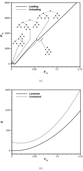
2.3 Martensite-to-martensite transition example . . . 43

2.4 Simple shear example . . . 45

2.5 Schematic of boundary layer . . . 47

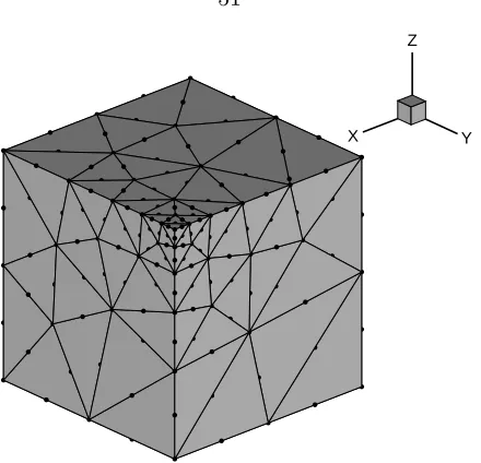
2.6 Computational domain and finite element mesh . . . 51

2.7 Unrelaxed indentation results . . . 52

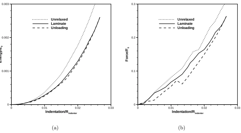
2.8 Indentation energies and forces . . . 53

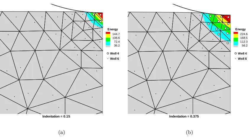
2.9 Laminate indentation results . . . 54

3.1 Three-well unrelaxed energy . . . 59

3.2 Tree representation of a solution to three rank-one connected wells . . . 60

3.3 Three-well relaxation . . . 62

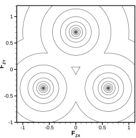
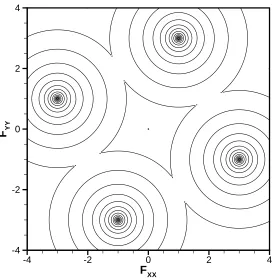
3.4 Four-well unrelaxed energy . . . 63

3.5 Diagram of the four-well problem . . . 64

3.6 Tree representation of analytic solution to the four-well problem . . . 65

(10)

3.8 Diagram of a solution of the four-well problem . . . 68

3.9 Incremental four-well relaxation . . . 70

3.10 Four-well relaxation along a path between two wells . . . 71

3.11 Graph of a numeric solution to the four-well problem . . . 72

3.12 Diagram of an incremental solution of the four-well problem . . . 73

3.13 Relaxation of nematic elastomer model . . . 76

3.14 Phase diagram of polycarbonate model . . . 80

3.15 3-D stress-strain diagram of polycarbonate model . . . 82

3.16 Energy of polycarbonate model in pure shear . . . 83

3.17 Polycarbonate model stress-strain response in pure shear and tension . . . . 83

4.1 Experimental stress-strain curves for Cu-Al-Ni . . . 90

4.2 Experimentally obtained microstructures . . . 90

4.3 Initial single material point response for Cu-Al-Ni tension test . . . 93

4.4 Finite element mesh of test specimen . . . 94

4.5 Stress-strain response of finite element simulation . . . 95

4.6 Tree representation of an austenite–twinned martensite microstructure . . . 96

4.7 Comparison of explicit austenite–martensite transformation . . . 97

4.8 Computed stress-strain curves . . . 98

(11)

List of Tables

1.1 Twinning relation vectors for Cu-Al-Ni . . . 7

3.1 Three-well initial guess forN . . . 60

4.1 Cu-Al-Ni experimental orientations . . . 90

4.2 Summary of Cu-Al-Ni experimental results . . . 92

(12)

Chapter 1

Introduction

A central problem in mechanics concerns the prediction of material processes on multiple

length scales and their cumulative effect on material behavior. Constitutive models that

incorporate effects from several length scales are important tools, both in circumstances in

which the model is directly applicable, and in the development of high fidelity models at

larger scales.

The research detailed herein is concerned with the computation of microstructures

re-sulting from the optimization of nonconvex energy functionals. This problem has

mathe-matical interest in its own right, but the present work will focus on applications to solid

mechanics. In particular, the algorithm developed will primarily be used in conjunction

with constitutive models of martensitic materials.

1.1 Martensitic materials

To begin, we review the theory of martensitic materials and compute some relevant

exam-ples. For more background refer to, e.g., [1, 11, 12, 17, 37, 58, 60] and references therein.

This overview shall largely follow the progression of Bhattacharya [17].

Martensitic materials, such as shape-memory alloys, are characterized by the occurrence

(13)

phase to one or more martensite phases upon a change in temperature or the

applica-tion of load. The resulting microstructures typically consist of complex arrangements of

several symmetry related variants. The composition, arrangement, and behavior of these

microstructures is the topic of this work.

In this class of materials, under proper conditions, the energy landscape imposed by

quantum mechanics renders the austenite phase unstable, instead favoring a different atomic

configuration. The prediction of this instability, while beyond the present scope, is accessible

to current methods in quantum chemistry such as Density Functional Theory [68].

Positing the existence of such phases, we require a formal description. Due to the

diffusionless nature of the transformation, there exists a linear mapping, corresponding to

a homogeneous deformation, that produces the lattice vectors of one variant from another

emartensite_i =U eaustenite_i (1.1)

whereU is the transformation matrix, and theei are lattice vectors. There will in general be several symmetry related martensite variants, each with a corresponding transformation

strain U_i. As an example, InTl undergoes a cubic to tetragonal transformation with the cubic austenite described by the transformation matrix

UA=I (1.2)

whereI is the identity matrix, and with three martensite phases

(14)

where diag() is a diagonal matrix and _{α, β_} describe the relative lengths of the lattice vectors. The three martensites thus correspond to stretching the cubic lattice by β in

each of the three coordinate directions in turn, with the remaining two lattice vectors both

deformed an amountα.

Frame indifference and material symmetry require the energy functional to satisfy

W(RT_PF RP) =W(F) (1.4)

where F is the deformation gradient and RP are the rotations that map the lattice onto itself (the point group of the lattice). Accordingly, the energy functional must reflect the

same symmetries embodied by the variants. This further implies that the related variants

must have the same energy. Frame indifference alone implies

W(RF) =W(F),R_∈SO(3), (1.5)

indicating that the energy of each variant is a well. Consequently, an energy model for

these materials is to assign similar energy wells to each martensite variant and another to

the austenite phase. The relative stability of each phase is accounted for by the value of

the energy at each well. Therefore, at the transformation temperature Tc all of the wells possess the same value of the energy at their minima, above Tc the austenite well is at a lower energy, while below the martensites are favored. This multiwell structure, imposed

by lattice symmetry, is nonconvex. As we shall see in the next section, these nonconvex

energies are responsible for the formation of microstructures.

Postulating the existence of microstructures, or recalling the experimental evidence [28,

(15)

phases to exist (without dislocations) the lattice vectors must satisfy continuity. Expressed

in terms of transformation matrices, we require that they share a common plane

RiUi−RjUj =a⊗N (1.6)

where{Ui,Uj} are the transformation strains of the two variants,N is the normal to the invariant plane, a is the shearing direction, and the variants are allowed to reorient via

{R_i,R_j_{} ∈}SO(3). Fixing the rotation of one variant and redefining a allows (1.6) to be

re-written as

RUi−Uj =a⊗N (1.7)

which is known as the twinning equation. This equation states that the deformationsRUi and Uj on either side of an interface arerank-one connected, i.e., they differ by the rank-one matrix a_⊗N. Note that equation (1.7) assumes that each variant is at its respective minimum energy deformation U—the ‘constrained’ theory of Ball and James [11, 12]—

which corresponds to the assumption that the material moduli are significantly larger than

the transformation stresses, and thus elastic deformations can be neglected. While the

deformations in general need not equal the transformation strain, compatability still insists

they be rank-one connected. Equation (1.7) does not indicate which microstructure will

form. However, with either sufficient creativity or with recourse to experimental results, it

can be used to explore possible compatible microstructures.

In anticipation of the work to follow, we shall derive several important microstructures

present in Cu-Al-Ni. This material undergoes a cubic to orthorhombic martensitic

transfor-mation and has, therefore, six variants in the martensitic phase. The defortransfor-mation undergone

(16)

be described by a stretch tensorUm, m= 1, . . . ,6. For Cu-Al-Ni, these are [28, 29]:

U1 =

       

ζ 0 0

0 ξ η

0 η ξ

       

, U2 =

       

ζ 0 0

0 ξ −η

0 ₋η ξ

       

, U3 =

       

ξ 0 η

0 ζ 0

η 0 ξ

        , (1.8)

U4 =

       

ξ 0 ₋η

0 ζ 0

−η 0 ξ

       

, U5 =

       

ξ η 0

η ξ 0

0 0 ζ

       

, U6 =

       

ξ ₋η 0 −η ξ 0

0 0 ζ

        , (1.9)

whereξ= 1.0425, η= 0.0194 andζ = 0.9178, and all components are referred to the cubic

axes of the austenitic phase.

1.1.1 Martensite–martensite laminate

An important microstructure observed experimentally [28, 29] is the laminar mixing of two

martensite variants, shown schematically in Fig. 1.1. Thus, given variants Ui and Uj, we

A

B

A

B

Figure 1.1: Schematic of a martensite–martensite microstructure with variants A and B.

wish to determine values ofR, a, andN that satisfy (1.7). Using Proposition 4 of Ball and

(17)

Equation (1.7) has a solution if and only if

λ1≤1 λ2 = 1 λ3≥1 (1.10)

where theλi, not all 1, are the ordered eigenvalues of

C =U−_jTU_iTUiU−_j1. (1.11)

There are then two solutions, given by

a = ρ



 s

λ3(1−λ1)

λ3−λ1

e1+κ

s

λ1(λ3−1)

λ3−λ1

e3



 (1.12)

N =

√

λ3−√λ1

ρ√λ3−λ1

−p1−λ1UT2e1+κ

p

λ3−1UT2e3

(1.13)

where κ =_±1,ρ ₆= 0 such that _|N_| = 1, and ei are the eigenvectors corresponding to λi.

R can then be found via (1.7).

The above procedure can be used to determine the required {R,a,N_} to satisfy (1.7) for two general deformations. Since we are following the constrained theory, as noted, the

above has been written with respect to the transformation strains U.

When the martensite variants are related via

Ui =RTUjR (1.14)

whereR is a plane of symmetry of the austenite and therefore is a 180◦ rotation about an

(18)

twinning equation again has two solutions, with the first solution given by [17]

a= 2 U−

T i eˆ

|U−_i Tˆe_|2 −Uieˆ

!

, N = ˆe, (1.15)

and a second solution

a=ρUieˆ, N = 2

ρ

e e₋U

T i Uiˆe |U_ieˆ_|2

, ρ= 2

ˆe−

UT_i Uiˆe |U_iˆe_|2

, (1.16)

whereρhas been calculated so that_|N_|= 1. For Cu-Al-Ni this calculation has been carried out by Bhattacharya, Li and Luskin [21]. The required rotation axes are given by ˆe=e/|e_|, with the vectore as in Table 1.1.

wells 1 2 3 4 5 6

1 e3 e1−e2 e1+e2 e1−e3 e1+e3

2 e₂ e₁+e₂ e₁₋e₂ e₁+e₃ e₁₋e₃

3 e₁₋e₂ e₁+e₂ e₃ e₂₋e₃ e₂+e₃

4 e1+e2 e1−e2 e3 e2+e3 e2−e3

5 e1−e3 e1+e3 e2−e3 e2+e3 e2

6 e1+e3 e1−e3 e2+e3 e2−e3 e1

Table 1.1: Vector e arising in the twinning relations for Cu-Al-Ni [21]. The vectors {e1,e2,e3} correspond to the cubic directions in the austenite phase.

These solutions can be classified as follows. When the solution for N is rational, as in

(1.15), the solution is referred to as a Type I twin. Conversely, solutions (1.16) where a is

rational are Type II twins. In some instances both a and N are rational—corresponding

to two solutions forR in (1.14)—referred to as a compound twin. For Cu-Al-Ni, the pairs

(19)

A

A Austenite

N

M

B

Figure 1.2: Schematic of an austenite–twinned martensite microstructure with martensite variants A and B.

1.1.2 Austenite–twinned martensite

Note that the solutions in Table 1.1 are between martensite variants only, and do not include

the austenite phase. Equation (1.7) has a solution involving austenite and martensite only

in very specific circumstances that do not occur for the vast majority of materials. Yet,

experimental evidence [74] clearly indicates the formation of an interface between austenite

and martensite. One such observed microstructure is illustrated in Fig. 1.2.

The interface between the martensites in the figure obeys (1.7) as above, but the interface

between this laminate and the austenite satisfies continuity only in an average sense. In

physical microstructures a transition region attains exact compatability at the interface [29,

50]. This average deformation gradient is

FM =λRUi+ (1−λ)Uj (1.17)

(20)

FM and austenite. Writing (1.7) for each of the interfaces shown in Fig. 1.2

RUi−Uj =a⊗N (1.18)

QFM −I =b⊗M (1.19)

whereI is the transformation strain of the austenite,_{Q,R_{} ∈}SO(3), and_{N,M_} (with corresponding {a,b_}) are defined in Fig. 1.2. The solution to (1.18) must correspond to one of the solutions obtained above. Theorem 7 of Ball and James [11] provides a solution

to (1.19), which can be stated as follows [17].

Let

δ = a_·Uj(U2j −I)−1N (1.20)

η = trace(U2_j)₋det(U2_j)₋2 +|a|

2

2δ . (1.21)

A solution exists if and only ifδ_{≤ −}2 and η_≥0. If δ=₋2 there is only one solution

λ = 1 2 1−

r

1 +2

δ

!

(1.22)

b = ρ



 s

λ3(1−λ1)

λ3−λ1

e1+κ

s

λ1(λ3−1)

λ3−λ1

e3



 (1.23)

M =

√

λ3−√λ1

ρ√λ3−λ1

−p1₋λ1e1+κ

p

λ3−1e3

(1.24)

(21)

matrix

C = (Uj+λN ⊗a)(Uj +λa⊗N) (1.25)

and whereρ is chosen so |M_|= 1,κ=±1, andQ is obtained from (1.19), while ifδ <−2 there is a second solution corresponding toλ_→(1₋λ).

Note that for each pair of variantsiandjthere are two solutions to (1.18) corresponding

to the two choices for κ in (1.12) and (1.13), each with up to four solutions to (1.18) and

(1.19). There are, therefore, eight possible austenite–twinned martensite solutions for each

pair of martensite wells. For the case of Cu-Al-Ni, all eight solutions exist for the 12 Type

I and Type II twins, with no solution for the three compound twins, resulting in a total of

96 solutions. A tabulation of these solutions is available in [74].

The two examples discussed above, while important, are by no means comprehensive.

For example, Bhattacharya has studied martensite wedges [14], while Chu and James have

observed a doubly laminated microstructure [29]. To determine which microstructure is

preferred, and to understand why they occur at all, one needs to look at energetics and the

issues involved with minimizing the nonconvex multiwell energies of such materials.

1.2 Nonconvex optimization

This section will give a brief overview of some of the issues involved in the minimization of

nonconvex energies such as the multiwell energy discussed above. The field is a large and

difficult one; for more background refer to [9, 11, 12, 17, 33, 37, 48, 54, 59, 60, 71].

Formally, we are interested in problems of the form

inf

y∈V I, I =

Z

Ω

(22)

where Ω_∈R3 _{is a deformable body,} _y₍_x_{) : Ω}_→R3 _{is a deformation with gradient} _F₍_x_{) =}

Dy(x), W(F) :R3×3 _→R_{, W} _≥_{0 is an energy density, and} _V _{is a suitable solution space.} While seemingly innocent, it is well known that such problems may be ill-posed if W is

nonconvex. Recall that a functionf(x) isconvex if

f(λa+ (1₋λ)b)_≤λf(a) + (1₋λ)f(b) (1.27)

∀a,b in the domain off, ∀λ∈[0,1].

We begin by reviewing the simple scalar case (see, e.g., [44, 59]) using the classical

approach. We are interested in obtaining the function y(x) that infimizes

I =

Z

f(x, y(x), y0(x))dx. (1.28)

In this case we can write the first variation

∂

∂λI(y+λη)

λ=0

= 0 (1.29)

whereη(x) is any admissible function. This results in

δI =Z η0(x)fy0+η(x)f_ydx= 0 (1.30)

where, e.g., fy=∂f /∂y. When integrated by parts this yields

δI =

Z

η

fy− d dxfy0

(23)

which must hold for allη. This finally leads us to the Euler equation for this case

fy = d

dxfy0 =fy0y0y

00₊_f

y0

yy0+fy0

x. (1.32)

Note that if fy0_y0 ≥0 this equation is elliptic, a necessary condition for a solution of (1.28)

to exist, indicating the importance of the convexity off with respect to y0.

The vectoral case is more complex. Following the direct method of the calculus of

variations [33], we demand that the integral I in (1.26) be finite and bounded from below.

We then seek minimizing sequences {yν} such that for some subsequence yν → ym and I(yν)& Im so that I(ym) = Im and I has a minimizer ym. This requires the (sequential)

weak lower semicontinuity of I

y_ν *y_⇒lim inf

ν→∞ I(yν)≥I(y) (1.33)

and reveals the crux of the problem: we need to determine ifI is weakly lower

semicontin-uous (l.s.c.) for the energy functional of interest.

Morrey [59] showed that an equivalent condition for the existence of minimizers is for

W to bequasiconvex, that is,

Z

Ω

W(F)dx_≤ Z

Ω

W(F +Dϕ(x))dx (1.34)

for allF andϕ(x). Hence, for a quasiconvex energy W, I is minimized by linear mappings

F [59].

(24)

polyconvex if

W(F) =g(M(F)) (1.35)

where g is a convex function of M(F), the vector of all minors of F. For F _∈ R3×3_,

M(F) = (F,cof(F),det(F)).

Another important concept of convexity is rank-one convexity, defined as

W(λa+ (1−λ)b)≤λW(a) + (1−λ)W(b) (1.36)

∀a,b in the domain ofW, _∀λ_∈[0,1], where rank(a₋b) _≤1. ThusW is rank-one convex if it is convex along all line segments with endpoints that differ by a rank-one matrix. Note

that this definition (1.36) implies that the total energy described by the rank-one compatible

energy wells discussed in _§1.1 is not rank-one convex (see, e.g., [33, 71]).

An important result is the relationship between the various notions of convexity, given

here as in Dacorogna [33]

W convex _⇒6⇐ W polyconvex _⇒6⇐ W quasiconvex _⇒6⇐ W rank-one convex

m m

I weakly lower

semicontinu-ous

Euler equations are

elliptic

(1.37)

where the last negative result is due to ˇSver´ak [80]. In one dimension all of these forms

are equivalent. In the present context, the most important implication of (1.37) is that the

multiwell energy density under discussion is not quasiconvex (and I is not l.s.c.), and thus

(25)

The concepts above are best illustrated with a simple example as discussed by

Bhat-tacharya and others [17, 60, 86]. Consider the one dimensional problem involving the

deformationy(x), x_∈(0,1) with gradientf =dy/dxand an energy

E(f) = (f(x)2−1)2 (1.38)

which has two wells atf =_±1. We will consider the total energy functional

I =

Z 1

0

(f(x))2−12+ (y(x))2

dx (1.39)

as in this simple example it is necessary to augmentE(f) to obtain the behavior of interest.

We wish to find a deformation y with zero energy. This requires

dy(x)

dx =f =±1 and y(x) = 0 (1.40)

which is obviously impossible. Yet, we can construct a minimizing sequence _{yν} = {y1, y2, . . . , yn} composed of the ‘sawtooth’ functions

yn(x) =

  

x, if 0< x < ₂1_n,

1

n−x, if

1

2n ≤x <

2 2n,

(1.41)

whereyn_{is extended periodically for}_x_∈₍ 2

2n,1), and is continuous. Obviouslyf =±1 =⇒ E(f) = 0, whiley→ 0 in anaverage sense: {yν} is aweakly convergent sequence. It is thus clear that limn→∞I(yn) = 0. Yet notice thatI is not weakly l.s.c., i.e.,{yν}*0 butI(0)> 0. Similar, less contrived, but more lengthy, examples can be found in the references above,

(26)

leads to the formation of microstructures which represent approximate solutions to the

problem (1.26).

One approach to the solution of such problems is via direct minimization of (1.26)

using, e.g., the finite element method. While straightforward, the preceeding discussion

indicates that this effort is in general essentially hopeless; the mesh would need to resolve

the microstructural details, and, further, would bias the solution. Nevertheless, as shown by

the indentation calculations of Tadmor et al. [81], and the small-scale finite element model

of the austenite–martensite interface of James et al. [50], this method can yield useful

results. Similarly, Collins et al. [30, 31, 58] solve the unrelaxed problem directly on a finite

element mesh, imposing affine boundary conditions consistent with the average deformation

gradient of a given laminate microstructure. This technique allows for the examination and

visualization of possible microstructures, but does suffer from mesh effects.

Alternatively, one can search for an effective or relaxed form of the energy that

ac-counts for the development of microstructure, and consequently would be quasiconvex. The

solution of this relaxed problem would be devoid of microstructure and would attain the

infimum.

Associated with each concept of convexity in (1.37) is an associated convex envelope

and convexification. The convex, polyconvex, quasiconvex, and rank-one convex envelopes

of the function f are defined as [33]

Cf = sup_{g_≤f :g convex_}

P f = sup_{g_≤f :g polyconvex_}

Qf = sup{g≤f :g quasiconvex} Rf = sup_{g_≤f :g rank-one convex_}

(27)

which with (1.37) implies

Cf ≤P f ≤Qf ≤Rf ≤f. (1.43)

Again following Dacorogna [33], given a functionf :Rn×m _→R_{∪ {}₊_∞}_{the convexification} is

Cf(A) = inf λi,Ai

(_nm₊₁ X

i=1

λif(Ai) : nm_X+1

i=1

λiAi =A

)

, _∀A_∈Rn×m_, _(1.44)

with an analogous expression for the polyconvexification. The quasiconvexification is

simi-larly computed via

Qf(A) = inf ϕ

1 |Ψ_|

Z

Ψ

f(A+Dϕ(x))dx

,_∀A_∈Rn×m_, _(1.45)

and is independent of the domain Ψ. Finally, following the construction of Kohn and

Strang [53, 54], the rank-one convexification can be written as

Rf0 =f (1.46)

Rk+1f(A) = inf

λ,A1,A2{

λRkf(A1) + (1−λ)Rkf(A2)} (1.47)

Rf = lim

k→∞Rkf (1.48)

where A = λA1 + (1 −λ)A2 and rank(A1 −A2) ≤ 1. This definition is equivalent to

theHN conditions discussed, e.g., by Dacorogna [33]. In the present setting, the rank-one convexification is the minimum energy attainable via recursive laminations of rank-one

con-nected deformations. Such a construction is referred to as asequential laminate, with a

(28)

the austenite–twinned martensite of_§1.1.2 is rank-two.

Returning to the solution of (1.26), it can be shown [33] that not only does the relaxed

problem attain the infimum, but the solution is also a minimizer to the original problem,

i.e.,

min

Z

Ω

QW(Dy(x))dx= inf

Z

Ω

W(Dy(x))dx. (1.49)

More precisely, as the unrelaxed problem need not attain its infimum, the minimizers of the

relaxed problem are weak limits of minimizing sequences of the original problem. A general

approach to obtainQW is thus highly desirable.

Unfortunately, the quasiconvexification is known only for a few problems (see, e.g.,

[37, 52, 54]), with no general algorithm available. Equation (1.46) does suggest a method

for obtaining RW, at least in the limit. However, RW 6⇒ QW in general, implying that this may only obtain a partial relaxation. We could therefore restrict ourselves to the study

of sequential laminates, which is the basis for the algorithm developed in the sequel.

Using this approach, Dolzmann introduced an algorithm [36, 39] that computes the

rank-one convexification of a function f _∈ Rm×n _{on a uniform grid, shown to converge to}

Rf as the mesh size decreases. The method operates via iterating over all matrices on the

grid and performing a convexification using tabulated rank-one directions at each point.

However, because of this tabulation the algorithm is only practical for f _∈ R2×2_{, and is} somewhat expensive: the presented numerical examples used, e.g., a mesh on [₋4,4]4 of 334 mesh points with 64 rank-one directions, requiring 75 million individual convexifications

per iteration over the grid.

More generally, Govindjee et al. [45–47] have implemented an algorithm based on a

(29)

of plasticity calculations, has been used to predict the experimental results of Shield [74],

and, further, offers insight into the relaxation of a generalN-variant energy. However, this

method is formulated using small strains, requires isotropic moduli, and cannot provide

microstructural details if desired.

Bhattacharya and Dolzmann [18, 19] have constructed approximate relaxed energy

func-tionals for the tetragonal-to-orthorhombic (two-well) and tetragonal-to-monoclinic

(four-well) cases. Their approach involved the determination of the quasiconvex hull of the

transformation strains—the (average) deformation gradients with zero energy. Given this

set, a quasiconvex energy functional was constructed that satisfied material symmetry, was

zero only on the quasiconvex hull with quadratic growth elsewhere, and reproduced the

material moduli.

An alternative approach to convexification is to solve the unrelaxed problem (1.26), but

consider a solution space consisting of ‘acceptable’ microstructures as described by

param-eterized measures orYoung measures. This method, first introduced by Young in 1937 [86],

describes the solution in terms of the local proportions (or probability distribution) of each

phase in an infinitesimally fine mixture. By their definition, Young measures

character-izeall minimizing sequences without requiring unnecessary details, and need not represent

laminates. For more detail, see [51, 60, 70, 71] and references within.

Ball and James have used parameterized measures to obtain an important result for the

two-well and three-well problems [11, 12]. Given boundary conditions corresponding to a

simple laminate

F =λU1+ (1−λ)RU2 (1.50)

(30)

stretches, they showed that the resulting microstructure is unique with Young measures

that correspond to a simple laminate if λ∈ (0,1). Bhattacharya, Li and Luskin [21] have obtained a similar result for cubic-to-orthorhombic transformations for nearly all values of

the transformation strains. Bhattacharya et al. also provide stability and error estimate

results useful in finite element calculations similar to those given by Li and Luskin [56, 57]

in the cubic-to-tetragonal case.

An example of a numerical application utilizing this method, Aranda and Pedregal [4]

have proposed an algorithm based on a finite element approximation of Young measures

resulting from the partial rank-one convexification of the energy [5]. They present results

for the two well problem which indicate some influence on mesh orientation.

For a survey of other numerical approaches consult the review article by Luskin [58].

Further background particularly relevant to the specific topic at hand will be provided in

later chapters.

Given the limitations of the current relaxation methods, there remains a need for an

efficient numerical algorithm for the relaxation of general multiwell energy densities. The

work presented here represents significant progress towards this end.

1.3 Outline

The next chapter, which first appeared as [7] (reproduced with permission), will present and

demonstrate an algorithm for computing the partial relaxation of a general multiwell energy

density via the explicit construction of a sequential laminate. The resulting microstructure

is at a local energy minimum, and is in static and configurational equilibrium. The present

author’s contribution included the finite element example calculations and requisite

(31)

The algorithm will be verified in Chapter 3 through comparison with several benchmark

problems. This provides the opportunity to both verify the correctness and understand the

limitations of the algorithm without the complications of an experiment.

In Chapter 4 the lamination algorithm will be used to model Shield’s Cu-Al-Ni tension

test experiment [74]. Shield obtained both the stress-strain response and microstructural

details for specimens at several orientations, enabling experimental verification of both the

response and microstructures obtained numerically.

(32)

Chapter 2

A constrained sequential

lamination algorithm

2.1 Introduction

Materials often are capable of adopting a multiplicity of crystal structures, or phases, the

relative stability of which depends on temperature, the state of stress, and other factors.

Under conditions such that several phases are energetically favorable, e.g., at the transition

temperature in martensitic materials, materials are often found to develop microstructure

in nature or in the laboratory. A central problem in mechanics concerns the prediction of

these microstructures and their effect on the effective or macroscopic behavior of materials,

including such scaling properties and size effects as may result from their formation and

evo-lution. When martensitic materials are modelled within the confines of nonlinear elasticity,

the coexistence of phases confers their strain-energy density function a multiwell structure

[16, 29, 40, 57]. The corresponding boundary value problems are characterized by energy

functions which lack weak sequential lower-semicontinuity, and the energy-minimizing

de-formation fields tend to develop fine microstructure [11, 12, 33, 60].

There remains a need at present for efficient numerical methods for solving macroscopic

(33)

at the microscale. One numerical strategy consists of attempting a direct minimization of

a suitably discretized energy function. For instance, Tadmor et al. [81] have applied this

approach to the simulation of nanoindentation in silicon. The energy density is derived from

the Stillinger-Weber potential by recourse to the Cauchy-Born approximation, and accounts

for five phases of silicon. The energy functional is discretized by an application of the

finite-element method. Tadmor et al. [82] pioneering calculations predict the formation of complex

phase arrangements under the indenter, and such experimentally observed features as an

insulator-to-conductor transition at a certain critical depth of indentation.

Despite these successes, direct energy minimization is not without shortcomings. Thus,

analysis has shown (see, e.g., [60] for a review) that the microstructures which most

ef-fectively relax the energy may be exceedingly intricate and, consequently, unlikely to be

adequately resolved by a fixed numerical grid. As a result, the computed microstructure is

often coarse and biased by the computational mesh, which inhibits—or entirely suppresses—

the development of many of the competing microstructures. By virtue of these constraints,

the numerical solution is often caught up in a metastable local minimum which may not

accurately reflect the actual energetics and deformation characteristics of the material.

In applications where there is a clear separation of micro and macrostructural length

scales, an alternative numerical strategy is to use a suitably relaxed energy density in

calculations [13, 27, 34, 45, 58]. In this approach, the original multiwell energy density

is replaced by its quasiconvex envelop, i.e., by the lowest energy density achievable by the

material through the development of microstructure. Thus, the determination of the relaxed

energy density requires the evaluation of all possible microstructures compatible with a

prescribed macroscopic deformation. The resulting relaxed energy density is quasiconvex

(34)

of microstructure and, thus, more readily accessible to numerical methods. In essence,

the use of relaxed energy densities in macroscopic boundary value problems constitutes a

multiscale approach in which the development of microstructure occurs—and is dealt with—

at thesubgrid level. The central problem in this approach is to devise an effective means of

determining the relaxed energy density and of integrating it into macroscopic calculations.

Unfortunately, no general algorithm for the determination of the quasiconvex envelop

of an arbitrary energy density is known at present. A fallback strategy consists of the

con-sideration of special microstructures only, inevitably resulting in a partial relaxation of the

energy density. For instance, attention may be restricted to microstructures in the form of

sequential laminates[34, 36, 52, 58, 63, 64]. The lowest energy density achievable by the

ma-terial through sequential lamination is known as therank-one convexification of the energy

density. Many of the microstructures observed in shape-memory alloys [29] and in ductile

single crystals [63] may be interpreted as instances of sequential lamination, which suggests

that the rank-one convexification of the energy coincides—or closely approximates—the

re-laxed energy for these materials. Ductile single crystals furnish a notable example in which

the rank-one and the quasiconvex envelops are known to coincide exactly [6].

In this paper we present a practical algorithm for partially relaxing multiwell energy

densities. The algorithm is based on sequential lamination and, hence, at best it returns

the rank-one convexification of the energy density. Sequential lamination constructions have

been extensively used in both analysis and computation [4, 5, 11, 16, 49, 52, 55, 58, 63]. All

microstructures generated by the algorithm are in static and configurational equilibrium.

Thus, we optimize all the interface orientations and variant volume fractions, with the result

that all configurational forces and torques are in equilibrium. We additionally allow the

(35)

The proposed lamination construction is constrained in an important respect: during

a deformation process, we require that every new microstructure be reachable from the

preceding microstructure along an admissible transition path. The mechanisms by which

microstructures are allowed to effect topological transitions are: branching, i.e., the splitting

of a variant into a rank-one laminate; and pruning, consisting of the elimination of

vari-ants whose volume fraction reduces to zero. Branching transitions are accepted provided

that they reduce the total energy, without consideration of energy barriers. By repeated

branching and pruning, microstructures are allowed to evolve along a deformation process.

The continuation character of the algorithm furnishes a simple model of metastability and

hysteresis. Thus, successive microstructures are required to be ‘close’ to each other, which

restricts the range of microstructures accessible to the material at any given time. In

gen-eral, this restriction causes the microstructures to be path-dependent and metastable, and

the computed macroscopic response may exhibit hysteresis.

The proposed relaxation algorithm may effectively be integrated into macroscopic

finite-element calculations at the subgrid level. We demonstrate the performance and versatility

of the algorithm by means of a numerical example concerned with the indentation of a

Cu-Al-Ni shape memory alloy [29] by a spherical indenter. The calculations illustrate the

ability of the algorithm to generate complex microstructures while simultaneously delivering

the macroscopic response of the material. In particular, the algorithm results in

force-depth of indentation curves considerably softer than otherwise obtained by direct energy

(36)

2.2 Problem formulation

Let Ω∈R3 _{be a bounded domain representing the reference configuration of the material.} Lety(x) : Ω_→R3_{be the deformation and}_F₍_x_{) =}_D_y₍_x_{) be the corresponding deformation} gradient. We denote the elastic energy density at deformation gradientF _∈R3×3_by_W₍_F_). We require W(F) to be material frame indifferent, i.e., to be such that W(RF) =W(F),

∀R_∈SO(3) andF _∈R3×3_{. In addition, the case of primary interest here concerns materials} such that W(F) is not quasiconvex. As a simple example, we may suppose thatW(F) has

the following special structure: Let Wi(F), i = 1, . . . , M be quasiconvex energy densities (see, e.g., [33] for a definition and discussion of quasiconvexity), representing the energy

wells of the material. Then

W(F) = min

m=0,...,MWm(F) (2.1)

i.e., W(F) is the lower envelop of the functions Wm(F).

A common model of microstructure development in this class of materials presumes that

the microstructures of interest correspond to low-energy configurations of the material, and

that, consequently, their essential structure may be ascertained by investigating the absolute

minimizers of the energy. However, the energy functionals resulting from multiwell energy

densities such as (2.1) lack weak-sequential lower semicontinuity and their infimum is not

attained in general [33]. The standard remedy is to introduce the quasiconvex envelop

QW(F) = 1

|Q_|u_∈Winf01,∞(Ω)

Z

Q

W(F +Du)dx (2.2)

(37)

the boundary, and Q is an arbitrary domain. Physically, QW(F) represents the lowest

energy density achievable by the material through the development of microstructure. The

macroscopic deformations of the solid are then identified with the solutions of the relaxed

problem

inf y_∈X

Z

Ω

[QW(Dy)₋f _·y]dx₋

Z

∂Ω2

¯

t_·y

(2.3)

where X denotes some suitable solution space, f is a body force field, t represents a

dis-tribution of tractions over the traction boundary∂Ω2, and the deformation of the body is

constrained by displacement boundary conditions of the form

y= ¯y on ∂Ω1 =∂Ω−∂Ω2. (2.4)

Thus, in this approach the effect of microstructure is built into the relaxed energyQW(F).

The relaxed problem defined by QW(F) then determines the macroscopic deformation.

In executing this program the essential difficulty resides in the determination of the

relaxed energy QW(F). As mentioned in the introduction, no general algorithm for the

determination of the quasiconvex envelop of an arbitrary energy density is known at present.

A fallback strategy is to effect a partial relaxation of the energy density by recourse to

sequential lamination [52, 58] and the use of the resulting rank-one convexification RW(F)

of W(F) in lieu of QW(F) in the macroscopic variational problem (2.3). We recall that

the rank-one convexification RW(F) ofW(F) follows as the limit [53, 54]

RW(F) = lim

(38)

PSfrag replacements

λ1

λ2

N1

N2

Figure 2.1: Example of a rank-two laminate. λ1 and λ2 are the volume fractions

cor-responding to levels 1 and 2, respectively, and N1 and N2 are the corresponding unit

normals.

whereR0W(F) =W(F) andRkW(F) is defined recursively as

RkW(F) = inf

λ,a,N{(1−λ)Rk−1W(F −λa⊗N) +λRk−1W(F + (1−λ)a⊗N),

λ_∈[0,1],a,N _∈R3_,_|_N_|_{= 1} _k _≥₁_.

(2.6)

In these expressions, λ and 1₋λ represent the volume fractions of the k-level variants,

N is the unit normal to the planar interface between the variants, and a is a vector (see

Fig. 2.1).

Unfortunately, a practical algorithm for the evaluation of the rank-one convexification

of general energy densities ‘on the fly’ does not appear to be available at present. Dolzmann

[36] has advanced a method for the computation of the exact rank-one convexification of

an arbitrary energy density in two dimensions. However, extensions of the method to three

dimensions are not yet available. In addition, the method requires the a priori tabulation

of RW(F) over all ofR2×2_{, which limits its applicability to large-scale computing.}

An additional complication arises from the fact that the cyclic behavior of martensitic

materials often exhibits hysteresis. Under these conditions, the response of the material

is path-dependent and dissipative, and, therefore, absolute energy minimization does not

(39)

con-sideration of entire deformation processes, rather than isolated states of deformation of the

material. A framework for the understanding of hysteresis may be constructed by

assum-ing that the evolution of microstructure is subject to a continuity requirement, namely,

the requirement that successive microstructures be close to each other in some appropriate

sense. This constraint restricts the range of microstructures which the material may adopt

at any given time and thus results in metastable configurations. The particular sequence

of metastable configurations adopted by the material may be path dependent, resulting in

hysteresis. The connection between metastability and hysteresis has been discussed by Ball,

Chu and James [10].

2.3 A sequential lamination algorithm

The problem which we address in the remainder of this chapter concerns the formulation

of efficient algorithms for the evaluation of RW(F), and extensions thereof accounting for

kinetics and nonlocal effects, with specific focus on algorithms which can be effectively

integrated into large-scale macroscopic simulations. We begin by reviewing basic properties

of sequential laminates for subsequent reference. More general treatments of sequential

lamination may be found in [14, 15, 52, 54, 58, 69].

Uniform deformations may conventionally be categorized as rank-zero laminates. A

rank-one laminate is a layered mixture of two deformation gradients, F−, F+ _∈ R3×3_. Compatibility of deformations then requiresF± to be rank-one connected, i.e.,

F+₋F−=a_⊗N (2.7)

(40)

of deformation. Let λ±,

λ−+λ+= 1, λ±∈[0,1], (2.8)

denote the volume fractions of the variants. Then, the average or macroscopic deformation

follows as

F =λ−F−+λ+F+. (2.9)

IfF and_{a, λ±,N_} are known, then the deformation in the variants is given by

F+ =F + λ−a_⊗N F− =F ₋ λ+_a_⊗_N

(2.10)

and, thus, F and _{a, λ±_,_N_} _{define a complete set of—deformation and configurational—}

degrees of freedom for the laminate. Following Kohn [52], a laminate of rank-k is a layered

mixture of two rank-(k−1) laminates, which affords an inductive definition of laminates of any rank. As noted by Kohn [52], the construction of sequential laminates assumes a

separation of scales: the length scale lk of the kth-rank layering satisfies lk lk−1.

Sequential laminates have a binary-tree structure. Indeed, with every sequential

lami-nate we may associate agraph Gsuch that: the nodes of Gconsist of all the sub-laminates

of rank less than or equal to the rankk of the laminate; and joining each sub-laminate of

order 1_≤l_≤k with its two constituent sub-laminates of orderl₋1. The root of the graph is the entire laminate. Two sequential laminates will be said to have the same structure

(alternatively, topology or layout) if their graphs are identical. Evidently, having the same

structure defines an equivalence relation between sequential laminates, and the set of all

equivalence classes is in one-to-one correspondence with the set_B of binary trees.

(41)

F

F+

S_S

S S

F−

ν1 F−+

S_S

S S

F−− ν2

λ+ λ−

λ−+ _λ−−

Figure 2.2: Example of a rank-two laminate. In this example, ν1 = λ−λ−+ and ν2 =

λ−λ−−.

associate a deformationFi. The root deformation is the average or macroscopic deformation

F. Each node in the tree has either two children or none at all. Nodes with a common

parent are called siblings. Nodes without children are called leaves. Nodes which are not

leaves are said to be interior. The deformations of the children of node i will be denoted

F±_i . Each generation of nodes is called a level. The root occupies level 0 of the tree. The number of levels is the rank k of the tree. Level lcontains at most 2l nodes. The example in Fig. 2.2 represents a rank-two laminate of order four. The three leaves of the tree are

nodesF+, F−+ and F−−. The interior nodes are F and F−. The children of, e.g., node

F− are nodesF−+ and F−−.

Compatibility demands that each pair of siblings be rank-one connected, i.e.,

F+_i ₋F−_i =ai⊗Ni, i∈ IG (2.11)

whereai∈R3,Ni∈R3, |N|= 1, is the normal to the interface betweenF−i andF+i , and IG denotes the set of all interior nodes. Letλ±_i ,

(42)

denote the volume fractions of the variantsF±_i with respect to nodei. Then, the deforma-tion of the parent variant is recovered in the form

Fi =λ−i F−i +λ+i F+i . (2.13)

IfFi and{ai, λ±_i ,Ni}are known for an interior nodei, then the deformation of its children is given by

F+_i =Fi+ λ−i ai⊗Ni

F−_i =Fi− λ+i ai⊗Ni.

(2.14)

Therefore, F and {ai, λ±_i ,Ni, i ∈ I} define a complete and independent set of degrees of freedom for the laminate. A recursive algorithm for computing all the variant deformations

Fi, i= 1, . . . , n from F and {ai, λ±i ,Ni, i∈ IG} has been given by [64].

We shall also need the global volume fractionsνl of all leavesl∈ LG, whereLGdenotes the collection of all leaves of G. These volume fractions are obtained recursively from the

relations

ν_i±=λ±_i νi, i∈ IG (2.15)

withνroot = 1 for the entire laminate, and satisfy the relation

X

l∈LG

νl= 1. (2.16)

Thus,νl represents the volume occupied by leaf l as a fraction of the entire laminate. The Young measure (e.g., [60]) of the laminate consists of a convex combination of atomsδFl(F)

(43)

The average or macroscopic stress of the laminate may be expressed in the form

P = X

l∈LG

νlPl (2.17)

where

P_l=W,F (Fl), l∈ LG (2.18)

are the first Piola-Kirchhoff stresses in the leaves. The average stress may be computed by

recursively applying the averaging relation

Pi=λ−P−i +λ+P+i , i∈ I (2.19)

starting from the leaves of the laminate. A recursive algorithm for computing the average

stress P from_{Pl, l∈ L}and {λ±i , i∈ IG}has been given by [64].

2.3.1 Microstructural equilibrium

We begin by investigating the mechanical and configurational equilibrium of sequential

laminates of a given structure. Thus, we consider an elastic material with strain-energy

densityW(F) subject to a prescribed macroscopic deformation F _∈R3×3_{. In addition, we} consider all sequential laminates with given graphG.

The equilibrium configurations of the laminate then follow as the solutions of the

con-strained minimization problem

GW(F) = inf

{ai,λ±i,Ni,i∈IG}

X

l∈LG

(44)

λ±_i _∈[0, 1], i_{∈ IG} (2.21)

|N_i|= 1, i_{∈ IG} (2.22)

where theF_lare obtained from the recursive relations (2.14). The effective or macroscopic energy of the laminate is GW(F). If W(F) is quasiconvex then it necessarily follows that

ai =0, ∀i∈ IG, and GW(F) =W(F).

It is interesting to verify that the solutions of the minimization problem (2.20) are

in both force and configurational equilibrium. Thus, assuming sufficient smoothness, the

stationarity of the energy with respect to all deformation jump amplitudes yields the traction

equilibrium equations

(P+_i ₋P−_i )_·Ni =0, i∈ IG. (2.23)

Stationarity with respect to all normal vectors yields the configurational-torque equilibrium

equations

[ai·(P+_i −P_i−)]×Ni =0, i∈ IG. (2.24)

Finally, stationarity with respect to all volume fractions yields the configurational-force

equilibrium equations

fi= (W_i+−W_i−)−(λ+_i P+_i +λ−_i P−_i )·(ai⊗Ni) = 0, i∈ IG (2.25)

wherefi is the configurational force which drives interfacial motion [75]. It bears emphasis that the leaf deformationsFlmay in general be arbitrarily away from the minima ofW(F), and thus the equilibrium equations (2.23) must be carefully enforced. In addition, the

(45)

the corresponding interface orientations. If all the preceding stationarity conditions are

satisfied, then it is readily verified that the average or macroscopic deformation (2.17) is

recovered as

P =GW,F (F) (2.26)

which shows thatGW(F) indeed supplies a potential for the average or macroscopic stress

of the laminate.

The case in which the energy density W(F) possesses the multiwell structure (2.1)

merits special mention. In this case, the minimization problem (2.20-2.22) may be written

in the form

GW(F) = inf

{ai,λ

±

i,Ni, i∈IG}

{ml∈{1,...,M}, l∈LG}

X

l∈LG

νlWml(Fl) (2.27)

λ±_i _∈[0, 1], i_{∈ IG} (2.28)

|N_i|= 1, i_{∈ IG} (2.29)

where m={ml∈ {1, . . . , M}, l ∈ LG} denotes the collection of wells which are active in each of the leaves. This problem may be conveniently decomposed into two steps: a first

step involving energy minimization for a prescribed distribution of active wells, namely,

GmW(F) = inf {ai,λ±i ,Ni, i∈IG}

X

l∈LG

νlWml(Fl) (2.30)

λ±_i ∈[0, 1], i∈ IG (2.31)

(46)

followed by the optimization of the active wells, i.e.,

GW(F) = inf

{ml∈{1,...,M}, l∈LG}

GmW(F). (2.33)

It should be carefully noted that the minimizers of problem (2.20-2.22) may be such

that one or more of the volume fractions λ±_i take the limiting values of 0 or 1. We shall say that a graph G is stable with respect to a macroscopic deformation F if at least one

minimizer of (2.20-2.22) is such that

λ±_i _∈(0, 1), _∀i_{∈ IG} (2.34)

and we shall say that the graph isunstable orcritical otherwise. The presence of sub-trees

of zero volume in an unstable graph is an indication that the graph is not ‘right’ for the

macroscopic deformationF, i.e., the graph is unable to support a nontrivial microstructure

consistent with F. Unstable graphs are mathematically contrived and physically

inadmis-sible, and, as such, should be ruled out by some appropriate means. This exclusion may

be accomplished, e.g., by the simple device of assigning the offending solutions an infinite

energy, which effectively rules them out from consideration; or by defining solutions modulo

null sub-trees, i.e., sub-trees of vanishing volume. In the present approach, we choose to

integrate the exclusion of null sub-trees into the dynamics by which microstructures are

evolved, as discussed next.

2.3.2 Microstructural evolution

The problem (2.20-2.22) may be regarded as a partial rank-one convexification of W(F)

(47)

follows from the consideration of all possible graphs, i.e.,

RW(F) = inf

G∈BGW(F) (2.35)

where, as before,_B is the set of all binary trees. In the particular case of energy densities of the form (2.1), we alternatively have

RW(F) = inf G∈B {ml∈{1,...,M}, l∈LG}

GmW(F). (2.36)

It is clear that this problem exhibits combinatorial complexity as the rank of the test

laminates increases, which makes a direct evaluation of (2.35) or (2.36) infeasible in general.

Problems of combinatorial complexity arise in other areas of mathematical physics, such

as structural optimization and statistical mechanics. Common approaches to the solution of

these problems are to restrict the search to the most ‘important’ states within phase space,

or importance sampling; or to restrict access to phase space by the introduction of some

form of dynamics. In this latter approach the states at which the system is evaluated form

a sequence, or ‘chain’, and the next state to be considered is determined from the previous

states in the chain. If, for instance, only the previous state is involved in the selection of

the new state, a Markov chain is obtained. In problems of energy minimization, a common

strategy is to randomly ‘flip’ the system and accept the flip with probability one if the

energy is reduced, and with a small probability if the energy is increased.

In other cases, the system possesses some natural dynamics which may be exploited

for computational purposes. A natural dynamics for problem (2.35) may be introduced

(48)

the microstructure along a deformation processes F(t). Here and subsequently, the real

variablet≥0 denotes time. A natural dynamics forG(t) is set by the following conditions:

1. G(t) must be stable with respect to F(t).

2. G(t) must be accessible fromG(t−_{) through a physically admissible transition.}

The first condition excludes laminates containing null sub-trees, i.e., sub-trees of zero

vol-ume. The second criterion may be regarded as a set of rules for microstructuralrefinement

and unrefinement.

In order to render these criteria in more concrete terms, we adopt an incremental

view-point and seek to sample the microstructure at discrete times t0 = 0, . . ., tn, tn+1, . . ..

Suppose that the microstructure is known at timetn and we are given a new macroscopic deformation Fn+1 =F(tn+1). In particular, let Gn be the graph of the microstructure at time tn. We consider two classes of admissible transitions by which a new structureGn+1

may be reached from Gn:

1. The elimination of null sub-trees from the graph of the laminate, orpruning.

2. The splitting of leaves, orbranching.

Specifically, we refer to branching as the process by which a leaf is replaced by a simple

laminate. The criterion that we adopt for accepting or rejecting a branching event is simple

energy minimization. Thus, letl ∈ LGn be a leaf in the microstructure at time tn, and let

Fn_l be the corresponding deformation. The energetic ‘driving force’ for branching of the leafl may be identified with

(49)

where R1W(F) is given by (2.6). We simply accept or reject the branching of the leaf

l∈ LGn according to whetherf n

l >0 orfln≤0, respectively.

In the particular case in which W(F) is of the form (2.1), the evaluation of R1W(F)

may be effected by considering all pairs of well energy densities, one for each variant.

However, since the well energy densitiesWm(F) are assumed to be quasiconvex and we rule out variants of zero volume, we may exclude from consideration the cases in which both

variants of the laminate are in the same well. The evaluation of R1W(F) is thus reduced

to the consideration of all distinct pairs of well energy densities.

The precise sequence of steps followed in calculations are as follows:

1. Initialization: InputF_n₊₁, setGn+1=Gn.

2. Equilibrium: Equilibrate laminate withGn+1 held fixed.

3. Evolution:

(a) Are there null sub-trees?

i. YES: _{Prune all null sub-trees,}GOTO _(2).

ii. NO: _Continue.

(b) Compute all driving forces for branching _{f_ln+1, l_{∈ LG}n+1}.

Letf_ln_max+1= maxl∈LGn+1f

n+1

l . Isflnmax+1 >0?

i. YES: _{Branch leaf} _l_max_, GOTO_(2).

ii. NO: _EXIT.

Several remarks are in order. The procedure just described may be regarded as a process

ofcontinuation, where the new microstructure is required to be close to the existing one in

(50)

arise at the end of each time step, there is no guarantee that this continuation procedure

delivers the solution of (2.35) for all t≥0. However, metastability plays an important role in many systems of interest, and the failure to deliver the absolute rank-one convexification

at all times is not of grave concern in these cases. Indeed, the continuation procedure

described above may be regarded as a simple model of metastability.

In this regard, several improvements of the model immediately suggest themselves. The

branching criterion employed in the foregoing simply rules out branching in the presence of

an intervening energy barrier, no matter how small, separating the initial and final states.

An improvement over this model would be to allow, with some probability, for transitions

requiring an energy barrier to be overcome, e.g., in the spirit of transition state theory and

kinetic Monte Carlo methods. However, the implementation of this approach would require

a careful and detailed identification of all the paths by which branching may take place, a

development which appears not to have been undertaken to date.

2.4 Illustrative examples

As a first illustration of the sequential lamination algorithm presented in the foregoing,

we apply it to a simple model of a Cu-Al-Ni shape-memory alloy, a material which has

been extensively investigated in the literature (cf. [11, 12, 29, 58], and references therein).

Photomicrographs taken from the experiments of Chu and James [29] (also reported by [58])

reveal sharp laminated microstructures, often of rank two or higher. In order to exercise

the algorithm, in the examples that follow we simply take the material through a prescribed

(51)

2.4.1 Material model

Cu-Al-Ni undergoes a cubic to orthorhombic martensitic transformation and has, therefore,

six variants in the martensitic phase described by the transformation stretches given by (1.8)

and (1.9). For purposes of illustration of the sequential lamination algorithm we adopt a

simple energy density of the form (2.1), with well energy densities

W0(F) = 1

8(F

T_F ₋_I₎_C

0(FTF −I) (2.38)

for the austenitic phase, and

Wm(F) = 1 8[(F U

−1

m )T(F U−m1)−I]Cm[(F Um−1)T(F U−m1)−I], m= 1, . . . ,6 (2.39)

for the martensitic phases. In these expressions C_m_, _m_{= 0}_{, . . . , M}_{, are the elastic moduli} at the bottom of the variants. These are (in MPa) [79, 85]

C₀₌        

C11 C12 C12 0 0 0

C12 C11 C12 0 0 0

C12 C12 C11 0 0 0

0 0 0 C44 0 0

0 0 0 0 C44 0

0 0 0 0 0 C44

        (2.40)

whereC11= 141.76, C12= 126.24 andC44= 97 and

C₁₌        

C11 C12 C13 0 0 0

C12 C22 C23 0 0 0