Path Planning with Real Time Obstacle Avoidance

Path Planning with Real Time Obstacle Avoidance

Durgesh Kumar Gupta

Amity University NOIDA(UP)

Anant Kumar Jaiswal

Amity University NOIDA(UP)

ABSTRACT

One of the most important areas of research on mobile robots is that of their moving from one point in a space to the other and that too keeping aloof from the different objects in their path i.e. real time obstacle detection. This is the basic problem of path planning through a continuous domain. For this a large number of algorithms have been proposed of which only a few are really good as far as local and global path planning are concerned as to some extent a trade of has to be made between the efficiency of the algorithm and its accuracy. In this project an integrated approach for both local as well as global path planning of a robot has been proposed. The primary algorithm that has been used for path planning is the artificial Potential field approach [1] and a* search algorithm has been used for finding the most optimum path for the robot. Obstacle detection for collision avoidance (a high level planning problem) can be effectively done by doing complex robot operations in real time and distributing the whole problem between different control levels. This project proposes the artificial potential field algorithm not only for static but also for moving obstacles using real time potential field values by creating sub-goals which eventually lead to the main goal of the most optimal complete path found by the A* search algorithm. Apart from these scan line and convex hull techniques have been used to improve the robustness of the algorithm. To some extent the shape and size of a robot has also been taken into consideration. The effectiveness of these algorithms has been verified with a series of simulations.

General Terms

Path planning approaches, search Algorithms

Keywords

Obstacle, search, hit point, leave point, path, approaches

1. INTRODUCTION

Problem of Path planning is as old as other various problems of robotics. The mainly focused area of research is that of real time obstacle avoidance with finding a most optimal path for the robot to move from the source point to the destination. For this there are a lot of algorithms, some just stop the robot at a safe distance from the obstacle to avoid the collision, some enable the robot to detour the obstacles. This particular approach not only detects the obstacle, but also takes in to consideration the size of the obstacle and the robot both to make sure that the whole dimension of the robot does not collide with any of the obstacles and it moves smoothly towards the goal position moving along the obstacle till it is in its path and then again resuming its direction of motion towards the target.

In case of autonomous path planning the robot assumes an environment in which it considers the presence of both the known or static and unknown or moving obstacles. This helps in effective path planning in which both a global map [2] (for

avoidance of known obstacles) and a local map (for real time obstacle detection and avoidance) are maintained. This project however concentrates on maintaining both global and local maps.

2. LITERATURE REVIEW

Path planning has got a lot of contributions from various researchers. Some of the several approaches for path planning are that of wall-following method [3, 4, and 5], edge detection method [6 and 7], hit and leave point approach [8], Histogramic in motion mapping approach [9] etc. In case of wall following method the robot starts from an initial position and then moves towards the nearest point along the wall and keeps on moving along it until it reaches the goal point. In case if an obstacle comes in the path of the robot it considers the sides of the obstacle as a wall and thus moves along it until it resumes to the original course in order to finally reach the goal point. In some other techniques edge detection mechanism is used. In this the robot takes in to consideration the vertical edges of the obstacle, for each edge the line connecting them is considered as the boundary of the robot and the robot tries to move along that boundary. One of the traditional approaches is that of hit and leave points using ultrasonic sensors in which as soon as an obstacle comes in front of the robot, it considers two points, one between itself and the obstacle (Hit point „H‟) and the other on the other side of the obstacle (Leave point „L‟) in such a way that line HL is in direction of the path from the source to the destination. Thus the robot starts from the hit point, moves along the obstacle while maintaining a safe distance, till it reaches the leave point.

3. PREVIOUS APPROACHES

3.1

Hit and Leave point approach.

In the techniques which follow Hit and Leave point approach, there a great possibility for the robot to get stuck in a kind of vicious circle when the obstacle is very thick (more than the range of the sensor being used). In such a case the robot adjusts a hit point correctly but in case of a leave point it is somewhere inside the obstacle. Due to this the robot keeps on moving along the obstacle to find the leave point and hence

gets stuck. Thus this algorithm is restricted to very thin obstacles. But this kind of a problem is not at all faced in the algorithm given in this paper.

3.2 Edge Detection approach.

3.3 Grid Approach

Unlike algorithms that maintain a certainty grid it doesn't have to maintain any such complex grids and hence is free from those complex calculations. Due to this reason this algorithm is quite fast and helps in faster movement of the robot.

The entire document should be in Times New Roman or Times font. Type 3 fonts must not be used. Other font types may be used if needed for special purposes.

4. PATH PLANNING AND OBSTACLE

AVOIDANCE

Path planning is concerned with the problem of moving a robot from an initial configuration to a goal configuration. The resulting route may include intermediate tasks and assignments that must be completed before the robot reaches the goal. Path planning algorithms can be classified as either global or local. Global path planning takes in to account all the information in the environment when finding a route from the initial position to the final goal configuration. Local planning algorithms are designed to avoid obstacles within a close vicinity of the entity.

Path planning includes both point-to-point and region filling operations. Point-to-point path planning looks for the best route to move an entity from point A to point B while avoiding known obstacles in its path, not leaving the map boundaries, and not violating the entity's mobility constraints. This type of path planning is used in a large number of robotics and gaming applications such as finding routes for autonomous robots, planning the manipulator's movement of a stationary robot, or for moving robots to different locations in a map to accomplish certain goals in a gaming application. While point-to-point operations are appropriate for some applications, they do not always produce the desired route for tasks such as vacuuming a room, plowing a field, or mowing a lawn. These types of tasks require region filling path planning operations that are defined as follows:

1) The mobile robot must move through an entire area, i.e., the overall travel must cover a whole region.

2) The mobile robot must fill the region without overlapping paths.

3) Continuous and sequential operation without any repetition of paths is required of the robot.

4) The robot must avoid all obstacles in a region.

5) Simple motion trajectories (e.g., straight lines or circles) should be used for simplicity in control.

6) An optimal path is desired under the available conditions. [13]

Both types of planning operations require searching through all the possible routes to find the most optimal, or efficient route among all the possibilities. Some search algorithms [14] work from the simplest to the more robust algorithms for searching a graph to find efficient routes. For e.g.: Breadth-first search, Depth-first search, Iterative-deepening search, Best-first search, A* search.

5. BASIC APPROACHES OF PATH

PLANNING

Due to the great importance of path planning in the field of motions planning for mobile robots a lot of approaches have been proposed which have their own merits and demerits. Different

approaches currently available for path planning can be classified in the following two broad categories

5.1 Model Based

 Polyhedral Obstacle model

 Free space decomposition

 Orthogonal space decomposition

 Grid model

 Potential field approach

5.2 Sensor Based

In this the sensed data is recorded on a grid map. Obstacles are represented by cells in the map. The value in the map determines whether there exists an obstacle or not.

Based on these models many algorithms have been proposed. These algorithms are

 Wall Following methods

 RRT Algorithms

 Edge detection techniques

 Hit and leave point approaches

 Genetic Approaches

 Grid Methods

 Potential field

6. RESEARCH DESCRIPTION

due to a large number of hit points and no leave point due to large thickness of the obstacle.

Hence keeping in mind these algorithms along with their advantages and disadvantages, this project discusses an approach which is quite effective in terms of finding an optimal path and accurate in terms of obstacle detection and avoidance.

6.1

Description of some previous Algorithms

6.1.1 Basic RRT Algorithm

In essence, an RRT planner searches for a path from an initial state to a goal state by expanding a search tree. For its search, it requires the following three domain-specific function primitives:

First, a function that calculates a new state that can be reached from the target state by some incremental distance (usually a constant distance or time), which in general makes progress toward the goal. If a collision with an obstacle in the environment would occur by moving to that new state, then a default value is returned to capture the fact that there is no “successor” state due to the obstacle. In general, any heuristic methods suitable for control of the robot can be used here, provided there is a reasonably accurate model of the results of performing its actions.

The heuristic does not need to be very complicated, and does not even need to avoid obstacles (just detect when a state would hit them). However, the better the heuristic, the fewer nodes the planner will need to expand on average, since it will not need to rely as much on random exploration. Next function needs to provide an estimate of the time or distance (or any other objective that the algorithm is trying to minimize) that estimates how long repeated application of first function would take to reach the goal.

Finally a function, that returns a state drawn uniformly from the state space of the environment.

6.1.2 Genetic Approach

The evolutionary procedure employed in the simulations consists in programming a standard genetic algorithm (GA) system, as described by Goldberg [11], to evolve the Robot steps controller.

This implementation is a new approach to the path-planning problem, representing each chromosome as a group of basic attitudes. These attitudes define the robot‟s movements in agreement with the feedback generated by its environment. Each feedback, which is used as input to the system, is based on the sensors reading and on the robot‟s direction to its goal location.

6.1.3 Histogramic in motion mapping

HIMM uses a two-dimensional Cartesian histogram grid for obstacle representation. Like the certainty grid, each cell in the histogram grid holds a certainty value (CV) that represents the confidence of the algorithm in the existence of an obstacle at that location. The histogram grid differs from the certainty grid in the way it is built and updated. This procedure is computationally intensive and might impose a time-penalty on real-time execution by an onboard computer.

6.1.4 Hit and Leave Point approach

In this approach the robot moves in the straight line along the path between the starting node and the end node. As soon as an obstacle comes in path of the robot it creates a hit point just in between the obstacle and itself and a leave point just at a side opposite to hit point along the path between the start and the end node on the other side of the obstacle. It starts from the hit point, decides randomly for the direction to move and then moves along

the side of the obstacle until it finds the corresponding leave point. After that it is again directed towards the goal point as before.

6.2 Description of different algorithms

implemented

6.2.1

The complete algorithm for path planning is based mainly on the potential field approach, along with the supporting convex hull and scan line algorithms for calculating the potentials of different points in order to make the robot move on a path directed towards the goal along with real time obstacle detection.

6.2.1.1 Initial input to the algorithm:-

The following are given as input to the algorithm in order to plan any path:-

(i) All the obstacles with coordinates of all the points of each obstacle.

(ii) Coordinates of the robot considering it as a polygon, in order to take into consideration its size also.

(iii) Size of the rectangular area in which planning has to be done.

(iv) Angle resolution, which decides the no, of directions in which the robot has to look for neighbours if any.

6.2.2 For Global Map:-

6.2.2.1 Assumptions

Albeit the algorithm works very well for almost all kinds of cases, there are still some assumptions that have been made, which do not affect the efficiency

(i) If a particular point is within the obstacle then it is assigned a negative potential.

(ii) If a particular is outside the boundary of the area to be considered (where path is to be planned) then it is assigned an infinite potential (a finite but very large value).

(iii) All other points are assigned a potential in increasing order starting with a zero from the goal point to the start point.

(iv) It starts with giving all the points within the bounds of the specified area an infinite potential

6.2.2.2 Modifying the obstacles

First of all the robot shape is integrated with each of the available obstacles in order to redefine the obstacles with a size larger than their original one, thereby making sure that the path that is planned for the robot is in such a way that whatever be the size of the robot, the planned path will be in such a way that the robot does not collide with the obstacle i.e. it is always at some distance from the obstacle.

6.2.2.3 Convex hull

Now considering this whole new obstacle (along with robot dimensions) as one, a convex hull is made for each of the modified obstacles in the following way.

N N

C

=

∑λ

j

p

j

: λ

j

≥ 0 for all j and

∑λ

j

=1

j=1 j=1

Fig 2. Expression to find convex hull

6.2.2.4 Scan line algorithm

Now each convex hull is scanned to assign a negative potential to all those points that lie inside the hull, this is done using the scan line algorithm.

In this algorithm first the complete width is scanned to see the total no of lines that form a part of any obstacle. Then between each odd and even line the following steps are performed while moving along the height:-

For each scan line crossing an obstacle, the algorithm locates the intersection points of the scan line with the obstacle edges. These intersection points are sorted from left to right and all the points lying between these points are stored and assigned a negative potential as has been set for the obstacles.

Some scan line intersections at the obstacle vertices require special handling. A scan line passing through a vertex intersects two obstacle edges at that position, adding two points to the list of intersections for the scan line. We can identify these vertices by 10 tracing around the obstacle boundary either clockwise or counter- clockwise order and observing the relative changes in the coordinates of the scan line as we move from one edge to the next.

If the end point y values of two consecutive edges monotonically increase or decrease, the middle vertex is counted as a single intersection point for any scan line passing through that vertex. Otherwise the shared vertex represents a local extremum (min or max) on the obstacle boundary, and the two edge intersections with the scan line passing through the vertex can be added to the intersection list.

The scan line algorithm can be summarized in following steps:-

1. Mark each edge of obstacle with direction.

2. Sweep scan line across layout.

3. At each point on scan line count the number of left hand and right hand edges to determine what rectangle that point is in.

Thus all those points that lie between all two points in the above list are assigned a negative potential which denotes an obstacle. Now starting with an initial point which is the start point of the path, all the nodes which have a positive finite potential that finally lead to the goal point are fed into the A* search algorithm which calculates the most optimal of all the available paths from the initial to the goal node.

Now it is checked for all the points that if they are in the specified area, they have infinite potential and they are not a part of the obstacle, then they are assigned a potential value in a sorted way starting with zero being assigned to the goal node and maximum potential to the starting node. The availability of a neighboring point is checked by passing the current point through the following matrix.

{

{ 0 , 0 , 1 }, Æ For +ve z direction

{ 0 , 1 , 0 }, Æ For +ve y direction

{ 1 , 0 , 0 }, ÆFor +ve x direction

{ 0 , 0 , -1 }, ÆFor -ve z direction

{ 0 , -1 , 0 }, ÆFor -ve y direction

{ -1 , 0 , 0 } ÆFor -ve x direction

}

This matrix yields 6 neighboring points. First their availability is checked for by making sure that they lie within the bounds of the work space and they do not have a negative potential field value. Thus all the available points from the start node to the final node are stored in a sorted manner and passed to the A* search algorithm to find the most optimal path for the robot.

Thus the main objective is to move the robot from the current position to a node which has a lower potential than the potential of the current node ultimately being directed towards the goal.

6.2.2.5 A* Search

It maintains two lists of nodes-open and close. Nodes on open list are nodes that have been generated but not expanded. Closed list are nodes that have been expanded and whose children are, therefore, available to the search program. It uses the heuristic function f(n)=g(n)+h(n), h(n)-distance/cost of start node to n node and g(n)- distance of n node to goal node. It maintains backtracking mechanism.

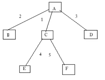
Fig 3 Tree to show A* search

In fig 2 let on expanding node A, we get three nodes B, C, D With heuristic function values as Shown. Since C is lowest , it will Be expanded to E and F. Out of B,E,F,D;B has Lowest value and so the search backtracks and explores node B and so on. It never follows a Particular branch of a tree. That node is explored which has the lowest heuristic value and hence in many cases (not always) it generates an optimum path between the initial and goal points, from all the available paths.

So if following are the forces present:-

1. FO= Repulsive Force by the obstacles which have negative

potential value.

2.FG = Attractive Force by the goal point due to least potential

value i.e. 0. This force is applicable to the sub-goal points in similar form.

3.FP = Repulsive Force by the previous points due to larger

4.FS= Repulsive Force by the surrounding points that have a

potential either infinity or larger than the potential of current node.

Thus the total force acting on the robot is as follows:-

FR = FO + FG + FP + FS

This force is overall attractive towards the goal point and hence leads the robot towards the goal point along the shortest and the most optimal path.

6.2.3 For Local Map

When the robot starts moving in the path that directs it towards the goal, it first computes potentials of all the points in the same way as for the global map, but divides the whole path into smaller number (which depends on the area in which path is to be planned) of parts and thereby converts the whole path into a series of sub-goals.

After reaching a sub goal a new path is again calculated to reach the next sub-goal by again assigning potentials to the nodes considering the current node as initial node and the next sub goal as the new goal node. Thus this takes care of the fact that if any obstacle is moving and it occupies a node initially unoccupied by global map, then that node is deleted from the list and the list is updated by defining a new path for that particular sub-goal.

Also if a sub goal is now unreachable due to movement of obstacles, then a new sub-goal is defined between the previous and the next sub-goal in such a way that there is no obstacle at that point. Also if a change occurs in the global map then again astar algorithm is applied to find the most optimal path between two sub- goals.

Thus the complete pseudo code for the approach is as follows:-

2.4 Procedure Find Path

Begin

Initialize qi = start point, qo = goal point

Assign Potential 0 to qo, -1 to obstacles using scan line, infinity to points outside the workspace and positive potentials in increasing order from goal to initial point to all other points

If Potential At (qi or qo) = infinity or Potential At (qi or qo) < 0

Return failure

Do if qi = qo return success

Else

Find best neighbor of qi with a* search depending on the potentials.

qi = nearest neighbor with a lower potential

While (true)

End

6.3 Advantages over conventional methods

This algorithm has many advantages over the other traditional approaches used for path planning and real time obstacle avoidance.

6.3.1. In the techniques which follow Hit and Leave point approach, there a great possibility for the robot to get stuck in a kind of vicious circle when the obstacle is very thick (more than the range of the sensor being used). In such a case the robot adjusts a hit point correctly but in case of a leave point it is somewhere inside the obstacle. Due to this the robot keeps on moving along the obstacle to find the leave point and hence gets stuck. Thus this algorithm is restricted to very thin obstacles. But this kind of a problem is not at all faced in the algorithm given in this paper.

6.3.2. In the edge detection approaches there might be a problem in accurate readings by the sensors. This results in distortion of the original shape of the obstacle and hence a misreading may lead to collision but in this algorithm no edge detection kind of a thing is done and hence it is free form the problems faced due to inaccuracies.

6.3.3. Unlike algorithms that maintain a certainty gird it doesn't have to maintain any such complex grids and hence is free from those complex calculations. Due to this reason this algorithm is quite fast and helps in faster movement of the robot.

6.3.4. Using this algorithm the robot does not have to stop for some time in front of the obstacles to take readings and calculating paths from it. It keeps on moving at its usual pace without stopping at all.

6.3.5. Unlike other conventional approaches this algorithm uses the A* search algorithm to find the shortest path (from among all the available paths) between two points.

7. RESULT AND TESTING

The algorithm has been tested by performing various simulations in complex as well as simple environments.

The main part of the algorithm is quite fast (faster than any of the traditional algorithms). All the computations are done very fast and hence its fetches fast and accurate results. Most part of the total time consumed is by the A* search algorithm which has a time and space complexity of O (b d), where b is the breadth and d is its corresponding depth.

But even then the total time consumed by the algorithm is very less.

Also there is a considerable amount of gain in the accuracy and efficiency of the algorithm.

Fig 4 Example path 1

Fig 5 Example path 2

Fig 6 Example path 3

Fig 7 Example path 4

Fig 8 Example path 5

8. CONCLUSION

The results clearly show that this algorithm is very robust in finding path in any kind of a

workspace. It is much better than any other conventional algorithm of path planning not only in terms of efficiency but also accuracy.

As far as obstacle detection and avoidance is concerned the potential field acting on the robot helps it to efficiently get rid of them and find a path between the initial and the goal point. Due to the presence of many forces together at a time on the robot, the robot reaches the destination point while being inside the defined workspace and keeping aloof from the obstacles in its path.

9. FUTURE SCOPE

The research in the field of mobile robots is growing very fast. At the present state the basis for enabling the mobile robots to imitate the human way of walking is almost ready. Now according to the current situation this is the best time that the different approaches developed by various researchers should be integrated and then implemented on a real robot in order to develop a robot that is able to maneuver easily in an environment which is real in terms of the environment i.e. with a lot of moving objects as well as on a rugged terrain where the robot has the task of not only moving but also balancing itself in order to move smoothly. Some work on the movement of a robot on a rugged terrain has been recently done [16].

Thus this work has a lot of scope for development as this forms the basis for the motion planning of mobile robots.

REFERENCES

[1] Oussama Khatib, "Real time obstacle avoidance for manipulators and mobile robots" The international journal of robotics research Vol 5, No 1 Spring 1986 © 1986 Massachusetts Institute of Technology.

[2] Borenstein, J. and Koren, Y., "Optimal Path Algorithms For Autonomous Vehicles." Proceedings of the 18th CIRP Manufacturing Systems Seminar, June 5-6, 1986, Stuttgart.

[3] Bauzil, G., Briot, M. and Ribes, P., "A Navigation Sub-System Using Ultrasonic Sensors for the Mobile Robot HILARE." 1st In.. Conf. on Robot Vision and Sensory Controls, Stratford-upon-Avon, UK., 1981, pp. 47-58 and pp. 681-698.

[4] Giralt, G., "Mobile Robots." NATO ASI Series, Vol. F11, Robotics and Artificial Intelligence, Springer-Verlag, 1984, pp. 365-393.

[5] Iijima, J., Yuta, S., and Kanayama, Y., "Elementary Functions of a Self-Contained Robot "YAMABICO 3.1”." Proc. of the 11th Int. Symp. on Industrial Robots, Tokyo, 1983, pp. 211-218.

[6] Borenstein, J., "The Nursing Robot System." Ph. D. Thesis, Technion, Haifa, Israel, 1987,.

[7] Borenstein, J. and Koren, Y., "Obstacle Avoidance With Ultrasonic Sensors." IEEE Journal of Robotics and Automation., Vol. RA-4, No. 2, 1988, pp. 213-218.

[8] Han-Pang Huang and Pei-Chien Lee “A real time algorithm for obstacle avoidance of autonomous mobile robots.” Robotics laboratory, Department of mechanical engineering, Ntional Taiwan University. Taipei, Taiwan 10764 (R.O.C.) 1991.

[9] ”Histogramic in-motion mapping for mobile robot obstacle avoidance” J. Borenstein , Member IEEE and Y. Koren, Senior Member IEEE Department of Mechanical Engineering and Applied Mechanics The University of Michigan, Ann Arbor, MI 48109

[10] James Bruce, Manuela Veloso"Real time randomized path planning for robot navigation" Computer Science department, Carnegie Mellon University.

[11] Goldberg, D.; Genetic Algorithms in Search, Optimization and Machine Learning , Addison-Wesley, 1989.

[12] Balakrishnan, K. and Honavar, V.; On sensor evolution in robotics. Proceedings of the First International Conference on Genetic Programming, Standford University, CA, pp. 455-460, 1996.

[13] Z. L. Cao, Y. Huang, and E. L. Hall, "Region Filling Operations with Random Obstacle Avoidance for Mobile Robots," Journal of Robotic Systems, vol. 5, no. 2, pp. 87-102, 1988.

[14] S. Russell and P. Norvig, Artificial Intelligence: A Modern Approach, Prentice Hall, 1995.

[15] Y. K. Hwang and N. Ahuja, "Gross Motion Planning - A Survey," ACM Computer Surveys, vol. 24, no. 3, pp. 219-290, 1992.

[16] Navigation of wheeled mobile robots on uneven terrain:- Niranjan Chakraborty & Ashtitva Ghosal ISPR-2004

Books Æ

[1] Robotics: Control, Sensing, Vision & Intelligence by King-Sun Fu, C.S. George Lee, King-King-Sun Fu, Ralph Gonzalez.