Reservoir Computing: Size and Connectivity Optimization using the "Worm Algorithm"

Reservoir Computing: Size and Connectivity

Optimization using the "Worm Algorithm"

A. S. Abdulrasool

Electrical Engineering Department, College of Engineering

Baghdad University, Iraq

S. M. Abbas

Electrical Engineering Department, College of Engineering

Baghdad University, Iraq

ABSTRACT

This work suggests an algorithm to find the optimum smallest value for Reservoir's Size (RS) and Connectivity Percent (CP) parameters in Reservoir Computing (RC) technique other than the gradient decent and evolutionary computation algorithms. This will help in reducing the required chip area and decreasing the number of multiplications before hardware implementation of RC.

General Terms

Reservoir Computing, Recurrent Neural Networks, Artificial Intelligence.

Keywords

Reservoir Computing optimization, Reservoir Size and Connectivity best values selection, Worm Algorithm, Reservoir tuning.

1. INTRODUCTION

Many researchers had tried to find mathematical rules that specify the relation between the input and output vectors' sizes from one hand and the number of layer and size of each layer on the other hand, in both Analog Neural Networks (ANN) and Spiking Neural Network (SNN) [1]. Even an approximation for such relation with large tolerance would be acceptable, but unfortunately such thing could not be found yet due to the nonlinearity of artificial neurons (both analog and spike neurons). This problem was inherited to RC technique in all its variants (Echo State Network (ESN), Backpropagation-Decorrelation (BPDC) and Liquid State Machine (LSM)) since the reservoir was built from artificial neurons in a recurrent manner.

In hardware implementation of Reservoir Computing (RC) technique, one should take care of Reservoir's Size1 (RS) (number of neurons in the Reservoir) and Recurrent Neural Network's (RNN) Connectivity Percent2 (CP); because they have a very strong influence (especially the size) on the Reservoir performance [2]. On the other hand, these parameters have a direct effect on the chip area; the size of reservoir is linearly proportional to the chip area if Application-Specific Integrated Circuit (ASIC) is used. Also it will require a Field Programmable Gate Array (FPGA) with larger size [3]. The increased connectivity of RNN will increase the wiring between neurons and thus increasing the number of multiplications [4].

In such cases one would tend to optimize such parameters using trial and error. The first algorithm that may come into the reader's mind is the gradient decent algorithm with all its variants [5]. If one want to apply the gradient descent algorithm to optimize the values of RS and CP in RC, then it

1

The Reservoir's size is measured in Neurons.

2

The Connectivity percent is unit less (percentage)

will requires to define a function that describes the relation between the RS and CP from one hand and performance3 of RC on the other hand in a certain task, this can be achieved by estimation. The problem of estimation it requires finding the Mean Square Error (MSE) at many values of CP and RS. This would not be a practical method because it will take too long time and a lot of mathematics due to the simulation of many reservoirs with different RS and CP, and then trying to find a function expresses the MSE in term of CP and RS using regression [6]. From this point it is concluded that it is impractical to implement the gradient decent algorithm with all their variants in the RC case.

The genetic algorithm may draw the attention to solve this optimization problem. The most appropriate genetic algorithm was used in [7] and [8] with a similar target. In that work Evolutional algorithm (EA) [9] and Evolutional Strategy (ES) [10] were used to find an ESN to control underwater robot motion in [11]. This was done in two phases, the first phase is to optimize parameters (RS, CP and Spectral radius) roughly using ES or EA, and then fine tuning the resulted ESN in the second phase. In the first phase, a simulation for ESNs with random triples (RS, CP and Spectral radius) will be carried out, then a parents with the lowest MSE will be chosen to generate the next generation of the triples (RS, CP and Spectral radius) by the mean of mutation. When some triples of latest generation had reached the specified MSE, the simulation is no longer implemented. Finally, the triples with the specified MSE or less are sorted in one class; one can choose an ESN from this class (usually the triple with the lowest RS and CP). In the second phase, the chosen ESN's inputs, output and reservoir weight matrices are tuned to reduce the MSE further.

Even thought this method is used to optimize not only the RS and CP, but also the Spectral radius. The required time and computations is very large (for the underwater robot controller design; which can be considered as a simple task, it had took about 7 days using MATLAB software package on a PC with 1.5 GHz processor and 512 MB RAM).

Instead of using gradient decent algorithm or the evolutionary computation, one may consider a directive trial and error method; since there is no need to know how the MSE behaves with respect to CP and RS.

The trial and error method will also require the simulation of a different reservoir with different RS and CP at each trial; this will consume time and calculations, so it will need to find an algorithm to minimize the trial's number as much as possible far away from the gradient decent algorithms. In such case one may not find the optimum parameters values,

3

but finding a low values that can give a low MSE may be considered as an achievement.

One can flow the path of the natural fruit worm to find the best4 values for RS and CP. When the natural fruit worm goes in a random point in a fruit (the edge of the fruit), from this random point it just tries to find the nearest points that have the highest benefits to it. Even though the fruit's size is relatively large to the fruit worm's size, but it is still can find the path to the best points without exploring the whole fruit's body. Creating an algorithm inspired by nature will be the aim of this paper. This algorithm will be explored in Section III. This algorithm the will be the "Worm Algorithm".

2.

FROM

MOTHER

NATURE

TO

ENGINEERING APPLICATION

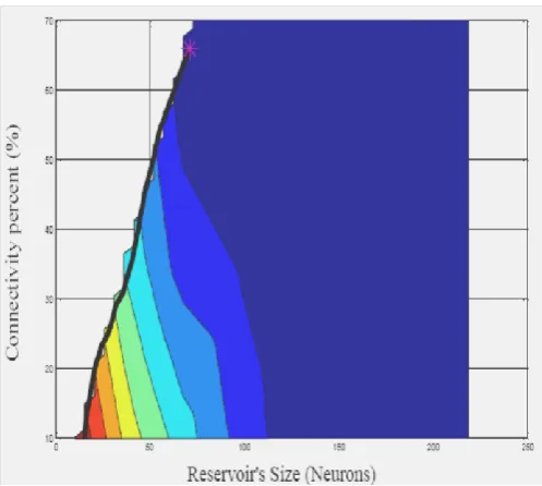
As mentioned in the introduction, this work had followed the path of the natural fruit worm. The way the fruit worm reaches its object (which is in this case is the nearest most useful part of the fruit) is by testing every points around her to find the best among them. After she finds it; she goes in that direction and searches for other points making the last selected point as a starting point for it. This seems intuitive method, but it should not be forget that the fruit tissue is somehow regular (i.e. the tissue is gradually changing from one point to others and not in a random manner); see Figure 1. The aim of these clarifications is to state the similarities between not only the natural fruit worm behavior and this algorithm but also between the fruit tissue (if a certain cross section is taken) and the plane formed by the RS and CP. A virtual worm can seek in that plane for the best points. The MSE surface is always simple in RC technique (i.e. consists of one peak and wide flat area), no matter what is the task it was chosen to implement [12].An example of RS CP-plane versus the MSE for "switchable attractor network" used in [13] is shown in Figure 2. This surface was obtained using the "Surface Fitting Toolbox" found in MATLAB software package version 7.10.0.499. This Toolbox had fitted points arranged in the xyz-coordinate system; the RS, CP and MSE represent the x-axis, y-axis and z-axis respectively.

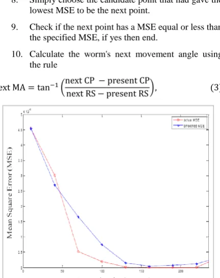
Table I shows these data according to which this surface was fitted; each column represents the coordinates of one point. It will be denoted by "MSE surface". Note that the MSE values were smoothed along the RS-axis for fixed value of CP; since one can obtain a MSE value deviate from its average with relatively small standard deviation if the network

Fig 1: Intensity image of an apple's cross section with "jet" color map.

4

The best may or may not be the optimum.

simulated many times with a fixed values of RS and CP5; see the simulated (actual MSE) and smoothed MSE along the RS with fixed CP of 10% in Figure 3. This step will guarantee more uniform surface. Assume that MSE surface represents a search area for a worm, the highest peak represents the lowest sweetness and their lowest areas represent the sweetest area. Now if a random point chosen in the MSE surface shown in Figure 2 to be the worm's insertion point, then this worm can certainly reach the most sweet area because there for every point there exist a path that's connects each point to the sweetest area (i.e. like the mountain surrounded by infinite flat area, when a rock breaks from any point it will roll to a flat position in a specific path). From this principle this algorithm was devised since most of the MSE surfaces in the RC technique are simple (have one peak and vast low flat areas).

3. WORM ALGORITHM

After the statement of the possibility to clone the behavior of nature to solve this problem. This idea should be translated to algorithm so it could be practically implemented. The worm algorithm can be summarized by the following steps and illustrations shown in Figure 4:

1. Specify the step size for each dimension (the increment in that parameter (RS and CP), when the worm moves from one point to another).

2. Chose the number of points that the worm can chose its next point from.

3. Specify the distance between these points.

4. Choose a random point to insert the worm and denote it the "present point" (PP) and a random angle that's the worm will move in its direction and denote it the "movement angle" (MA).

Fig 2: The MSE versus Reservoir Size Connectivity percent –plane

5

5. Find the coordinates of each point using the following rules

where the present RS and present CP are coordinates of PP in the RS CP-plane, and are certain functions (the next example will clarify them) and they are usually trigonometric functions, and is the angle between the line that connect the PP to the i-th point that the worm will choose from and the RS-axis.

6. Check if at least one point lies in the selected region (i.e. not all points lie in the region where the CP higher than RS, this region will be called the "forbidden region"). Exclude these points from selection. The remaining points will be called the "candidate points". Note that if all points lie in the forbidden region then one should increase or (decrease) the movement angle by an amount of ϑ or (-ϑ) if the worm's movement angle is greater than 135o _{or (less than 135}o_{) and repeat from step 5.}

7. Start to calculate the MSE at each candidate point by training the networks using the same teacher data.

8. Simply choose the candidate point that had gave the lowest MSE to be the next point.

9. Check if the next point has a MSE equal or less than the specified MSE, if yes then end.

10. Calculate the worm's next movement angle using the rule

Fig 3: Actual and smoothed MSE versus Reservoir size with fixed Connectivity of 10%.

11. Replace the PP by the next point and repeat from step 5. The next example will illustrate the Worm Algorithm's steps in more detail.

4. EXAMPLE

Consider the earlier mentioned switchable attractor network; it will be tried to obtain an ESN with MSE no more than 10-6 with RS and CP as low as possible with Spectral radius of 0.9.

4.1

Parameters initialization and

procedures:

The Procedure will be simulated using MATLAB software package. Using a PC with 1.5 GHz processor and 512 MB RAM. The simulation program's steps and parameters initialization are as follows:

1. Let the step size be 4 and 10 for RS and CP respectively (i.e. it is desired to bias the worm toward a high CP rather than a large RS).

2. Let the number of points that the worm can chose from be five.

3. Let the separation angle between a point and the next one with respect to the PP be 18o; see Figure 5. Then the worm's angle of sight will be

4. Let the insertion point (first PP) of the worm be (RS=10,CP=5), the initial MA and ϑ be 45o and 30o respectively..

5. Now let's find the coordinates of each point using (1) and (2), assume that

where 'nearest' means the nearest integer valueandi =1, 2, 3, 4, 5.

6. Find the candidate points and calculate the MSE at each candidate point and chose the point with the lowest MSE and make it the worm's next point and check if the MSE at this point is less or equal to 10-6, if so, end the program.

Table 1. Data used to fit the surface shown in Figure 2

RS 10 30 70 100 130 160 190 220 35 65 95

CP 10% 10% 10% 10% 10% 10% 10% 10% 35% 35% 35%

MSE × 10-3 4.5 2.7 1.7 0.74 0.14 0.04 .002 4×10-5 2 0.8 .05

RS 125 155 185 215 70 100 130 160 190 220

CP 35% 35% 35% 35% 70% 70% 70% 70% 70% 70%

Fig 4: Illustration of the Worm algorithm.

7. Calculate the worm's next MA using (3).

8. Replace PP by the next point, MA by next MA and repeat from step 5.

Note that the simulation program will not stop unless the MSE has reached the specified value or less.

4.2

Results

The simulation results are shown in Figure 6; where the black line and the pink star represent the worm's path and final position respectively.

The final position was (RS=71,CP=66), this took the worm to move over 14 points before it reaches this point.

The colored plane represents the projection of the MSE surface shown in Figure 2 on the RS CP-plane, the number of computations of the MSE is

The simulation period was 480 second. The number of

and the period of simulation can easily reduced just by increasing the step size (consider a 30 by 30), reducing the number of points that's the worm can choose from (consider 3 points) and/or increasing the worm's angle of sight.

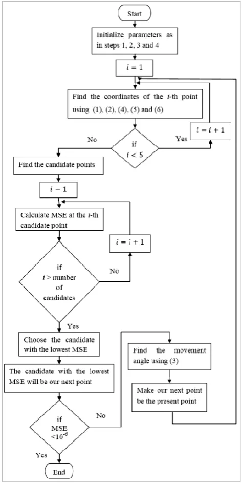
From Figure 6, it will be concluded that the worm had found the nearest point to the origin with a MSE equal or less than 10-6 to be its final position (i.e. excellent values for RS and CP for the switchable attractor network). Figure 7 shows a schematic flowchart of the simulation program's steps.

Fig 5: Points arangments and angles.

5.

CONCLUSIONS

AND

FUTURE

WORKS

The worm algorithm had given quite good result for the example in Section IV. Both short time and low number of computations are met in this algorithm; unlike the methods used in [7] and [8] even thought these methods were used to optimize the Spectral radius as well. It would be very useful if the designers consider using it to find the lowest RS and CP that can perform the required task before the hardware implementation, instead of making their decisions on experts' estimations. This means the integrated chips manufacturers can reduce the cost in an easy manner.

Also this algorithm can be used not only for RC applications but for other applications such as feed forward neural networks number of layers and number of neurons per layer reduction and any engineering problem that may need a trial

Fig 7: Shematic flowchart of the simulation program's steps.

and error solution. Note that this algorithm also can used to find the best values for more than two parameters.

We recommend for more working on this algorithm to make it faster, do fewer computations and more accurate. There are

some points the reader may consider if he wishes to develop this algorithm, these points are:

1. Make the step sizes variable with respect to the difference between the present and intended MSE, one can make large step sizes for slow changes if that difference is small and small step size for the opposite, consider linear or exponential relation between them.

2. Make the worm's angle of sight a function of the regularity of the MSE surface (i.e. increasing the angle of sight if the surface various sharply), the MSE surface's attributes can be estimated according

to variation of the calculated MSEs of the previous candidate points.

3. The same thing can be used for number of points that's the worm can chose from (i.e. increase the number of points that's the worm can chose from if the surface various sharply).

4. Many worms can be inserted at different points in the same MSE surface at the same time, so it can increase the choices and select the best from bests. 5. Including the Spectral radius to the optimization

process (i.e. optimizing the triple (RS,CP, Spectral radius)).

6. ACKNOWLEDGMENTS

Special thanks to Omama Abdulrazaq for very valuable discussions and to Electrical Engineering Department of Baghdad University.

7. REFERENCE

[1] Lukoševičius, M. and Jaeger, H. 2009. Reservoir computing approaches to recurrent neural network training. Science Review, vol. 3, pp. 127-149. [2] Abdulrasool, A. S. 2010. A Study of Reservoir

Computing: Echo State Network and Liquid State Machine. M.Sc. thesis, Electrical Engineering Department, Bghdad University.

[3] Verstraeten, D., Schrauwen, B., D'Haene M. and Stroobandt, D. 2006. The unified Reservoir Computing concept and its digital hardware implementations. In Proceedings of the 2006 EPFL LATSIS Symposium. [4] Schrauwen, B. 2008. Towards Applicable Spiking

Neural Networks. Doctrine assertion, Gent University of Technology.

[5] Zurada, J. M. 1992. Introduction to Artificial Neural Systems. West Publishing Company, New York, United States.

[6] Draper, N. R. and Smith, H. 1998. Applied Regression Analysis, Wiley-Interscience.

[7] Ishii, K., Van der Zant, T., Becanovic, V. and Ploger, P. 2004. Identification of motion with echo state network. OCEANS '04. MTTS/IEEE TECHNO-OCEAN '04 , vol. 3, pp 1205-1210.

[8] T. Van der Zant, V. Becanavic, K. Ishii, H. Kobiaka, P. Ploeger, "Finding Good Echo State Networks to control an Underwater Robot using Evolutional Computations", In A proceding volume from the 5th IFAC Symposium, 2004.

[9] Holland, J. H. 1975. Adaptation in natural and artificial systems. The University of Michigan Press, Ann Arbor, MI.

[10]Rudolph, I. 1991. Global Optimization by means of Distributed Evolutionary Strategies. In: Parallel Problem Solving from Nature, Schwefel, H. P. and Manner, R. Eds., PPSN, vol. 496 of Lecture Notes in Computer Science, pp 209-213.

[11]Fujii, T., Ura T. and Kuroda, Y. 1993. Mlission Execution Experiment with a Newly Develooed AUV the Twin-Burger. In: Proc. of the 8th UUST , pp 92-105. [12]Verstraeten, D., Schrauwen, B., D'Haene, M. and Stroobandt, D. 2007. An experimental unification of reservoir computing methods. Neural Networks , vol. 29 , pp. 391-403.