Explaining the US Bond Yield Conundrum

Munich Personal RePEc Archive

Explaining the US Bond Yield

Conundrum

Bandholz, Harm and Clostermann, Joerg and Seitz, Franz

February 2007

Online at

https://mpra.ub.uni-muenchen.de/2386/

FACHHOCHSCHULE

AMBERG - WEIDEN

FH

im Dialog

Weidener

Diskussionspapiere

Diskussionspapier No. 2

Februar 2007

Explaining the US Bond Yield Conundrum

Impressum

Herausgeber Prof. Dr. Horst Rottmann (FH Amberg-Weiden)

Prof. Dr. Franz Seitz (FH Amberg-Weiden)

Fachhochschule Amberg-Weiden, University of Applied Sciences, Abt. Weiden, Hetzenrichter Weg 15, D-92637 Weiden

Telefon: +49 961 382-0 Telefax: +49 961 382-110

e-mail: [email protected]

Internet: www.fh-amberg-weiden.de

Druck Hausdruck

Die Beiträge der Reihe "FH im Dialog: Weidener Diskussionspapiere" erscheinen in

unregelmäßigen Abständen.

Bestellungen schriftlich erbeten an: Fachhochschule Amberg-Weiden, Abt. Weiden, Bibliothek, Hetzenrichter Weg 15, D-92637 Weiden

Die Diskussionsbeiträge können elektronisch unter www.fh-amberg-weiden.de abgerufen werden.

Alle Rechte, insbesondere das Recht der Vervielfältigung und Verbreitung sowie der Übersetzung vorbehalten. Nachdruck nur mit Quellenangabe gestattet.

Explaining the US Bond Yield Conundrum

Harm Bandholz

, Jörg Clostermann*, Franz Seitz

January 2007

#

) Bayerische HypoVereinsbank *) University of Applied Sciences +) University of Applied Sciences Global Research Ingolstadt Weiden

Arabellastraße 12 Esplanade 10 Hetzenrichter Weg 15 D-81925 München D- 85049 Ingolstadt D-92637 Weiden

Germany Germany Germany

[email protected] [email protected] [email protected]

Abstract:

We analyze if and to what extent fundamental macroeconomic factors, temporary influences or more structural factors have contributed to the low levels of US bond yields over the last few years. For that purpose, we start with a general model of interest rate determination. The empirical part consists of a cointegration analysis with an error correction mechanism. We are able to establish a stable long-run relationship and find that the behavior of bond yields, even during the last two years, can well be explained. Alongside the more traditional macroeconomic determinants like core inflation, monetary policy and the business cycle, we also include foreign holdings of US Treasuries. The latter should capture the frequently mentioned structural effects on long-term interest rates. Finally, our bond yield equation outperforms a random walk model in different forecasting exercises.

Keywords: bond yields, interest rates, cointegration, inflation, forecasting

Deutscher Abstract:

Explaining the US Bond Yield Conundrum

1. Introduction

Long-term interest rates in Europe and in the US fell to all-time lows in the last few years.

And despite a rebound, they still have been traded at historically low levels in 2006,

especially in the US. This is even more remarkable as the economic environment during the

same time has been unfavorable for Treasuries: The US economy has so far been growing

above trend, the Fed has raised its target rate several times and core inflation has been

increasing since 2004.

In his February 2005 testimony before the Committee on Banking, Housing, and Urban

Affairs of the U.S. Senate, Alan Greenspan asserted: "For the moment, the broadly

unanticipated behavior of world bond markets remains a conundrum. Bond price movements

may be a short-term aberration, but it will be some time before we are able to better judge the

forces underlying recent experience." In the monthly report of April 2005, the ECB also stated

that macroeconomic fundamental factors alone cannot explain the development of long-term

interest rates and pointed to structural factors that are behind recent bond market

developments. "A number of changes in the regulatory environment for pension funds and life

insurance corporations appear to be under way in the euro area and the United States, which

aim to reduce the problems of mismatches between the duration of their assets and liabilities.

It is generally perceived that these regulatory changes will favor the purchase of bonds over

other asset classes by pension funds and life insurance corporations." (ECB, 2005, 23). As a

result of these changes and anticipatory effects of the proposed legislation, there may have

been an increase in the structural demand for bonds of longer maturities from institutional

investors which contributed to a bullish market.

While some of these more structural factors point to a possible permanent change in

long-term real interest rates, there are hints that other, more temporary market influences related to

speculative behavior may have played a role, too. The alleged widespread use of so-called

carry trades - borrowing at low short-term interest rates and investing in higher yielding,

longer-term maturities - appears to exploit market trends, and thus may have amplified the

downturn in long-term interest rates. Speculative flows of this sort, however, are likely to be

∗

reversed at some point and hence should not have a permanent effect on the level of long-term

interest rates. In addition, as Bernanke et al. (2004) pointed out, the massive purchases of

government bonds by Asian central banks probably have had a significant impact on

long-term bond yields in the US. According to the ECB (2006), quantitative estimates about the

yield impact of foreign reserve accumulation ranges from 30 to 200 basis points.

Moreover, recent empirical papers find tentative evidence that structural factors are at work.

Clostermann and Seitz (2005) developed a traditional US-bond yield model driven by

monetary policy, the business cycle and inflation expectations. Although the out-of-sample

performance of their model was good, they conclude that, "there are hints of some instabilities

in the last years". Kozicki and Sellon (2005, 29) suggest "that the key factor behind the

conundrum is a large reduction in the term premium." Bandholz (2006) shows that the

unexplained part of his US bond model increases to values not seen in the past when data for

2006 are included. Moreover, Rudebusch et al. (2006) confirm on the basis of empirical

no-arbitrage macro-finance models of the term structure "that the recent behavior of long-term

yields has been unusual - that is, it cannot be explained within the framework of the models."

On the other hand, Fels and Pradhan (2006) find that a conundrum no longer exists. They

state that "a drop of bond yields below their fair value such as the one seen last year did not

represent a break with past pattern and, as such, did not require a new paradigm to explain it.

In fact, our statistical tests suggest that the relationship between bond yields and our three

fundamental factors (i.e., the real federal funds rate, inflation expectations and inflation

volatiltiy, BCS) did not change significantly in recent years. And, as in previous episodes of

overvaluation in the bond market, actual bond yields eventually corrected since the fall of

2005, rising towards their fundamental fair value."

To find out whether fundamental macroeconomic, temporary or more structural factors have

been at work we proceed as in Clostermann and Seitz (2005). First, we discuss which

fundamentals should theoretically determine bond yields. These are essentially the three

macroeconomic factors identified by Dewachter and Lyrio (2006) and Diebold et al. (2006):

monetary policy, inflation expectations and the business cycle which are augmented by

structural factors.1 Next, we estimate an interest rate model for ten-year (10Y) US Treasury

notes and analyze whether there are hints of unexplained interest rate developments and of

overvaluations of the bond market in recent years. In doing so, we also derive a "fair value"

1

for the yield of 10Y Treasuries which we compare to actual developments to get an idea of the

magnitude of the evolving disequilibrium. This helps to answer the question whether the bond

market overvaluation in 2005/06 has been unusually strong in a historical context.

Furthermore, we perform some out-of-sample forecasting exercises of our preferred model

and compare it to a random walk model.

The existing empirical literature approaches the problem of bond yield determination in four

different ways. The first strand of literature looks for fundamental factors as explanatory

variables (see, e.g., Mehra, 1995; Caporale and Williams, 2002; Brooke et al., 2000; Durré

and Giot, 2005). The second approach uses high-frequency (in most cases daily) data to

analyze the reaction of yields to news or announcements (see, e.g., Monticini and Vaciago,

2005; Demiralp and Jordà, 2004). The third kind of models discusses the international

transmission of shocks with respect to bond markets (see, e.g., Ehrmann et al., 2005). And,

finally, the fourth approach combines bond yield modeling strategies from a finance and

macroeconomic perspective to get a comprehensive understanding of the whole term structure

of interest rates (e.g. Dewachter and Lyrio, 2006; Diebold et al., 2006). Our view is a

synthesis of especially 1 and 3, but also partly borrows from 4.

2. What determines interest rates? Some theory

Generally, interest rates should be determined by the supply of and the demand for loanable

funds and their determinants including the production opportunities in the economy

(depending on technological developments), the rate of time preference, risk aversion and the

relative returns of alternative investments. Ideally, this would necessitate a dynamic and

stochastic general equilibrium model of the economy with supply and demand conditions

derived from first principles.2 So far, however, DSGE models with an elaborated financial

sector are still in their infancy.

Therefore, and in line with other studies, our analysis starts with a general model for the term

structure of interest rates:

(1) l = s+ ( , )

t t t

r r rp l c

where rlt is the real long-term rate, rst is the real short-term rate, l and s denote the terms of the

bonds, ct is a set of variables that influences investors’ risk attitudes and rp is the function

2

defining that influence which gives us the term or risk premium in rlt (Caporale and Williams,

2002, 121).3

To make (1) suitable for empirical work, we need information on the specifics of rp.

Following Breedon, Henry and Williams (1999), Caporale and Williams (2002) and others, ct

is a catch-all variable for risks arising from macroeconomic policy developments.

Specifically, we define

(2) rtl = ßrts+γrp l bc etc( , t, t),

t

where bc is a variable capturing the state of the business cycle. In "etc" different further

factors influencing the macroeconomic environment could be subsumed. In this direction,

Caporale and Williams (2002) as well as Paesani et al. (2006) analyze the fiscal position.

Jordá and Salyer (2003) ask whether the liquidity situation helps to explain bond yields (see

also ECB, 2005, 23). Durré and Giot (2005) investigate whether stock market variables are

responsible for bond market developments. We decided to include an indicator variable which

has already been considered in the past, but in a different way than we do (see Warnock and

Warnock, 2005; Wu, 2005; Frey and Moëc, 2005). It refers to a changing structural demand

by foreigners for US Treasuries. A more concrete description and discussion are provided in

section 3.1.

(1) and (2) are specified in real terms. Two problems arise in this context (Caporale and

Williams, 2002, 122). First, real rates are not directly observable but have to be proxied for

empirical work. Second, the strength of the effect of expected inflation on nominal long-term

rates (il) is ambiguous. It might be a one-to-one relationship if the Fisher effect holds. This is

the case in all models in which the real interest rate does not depend on monetary variables

and monetary neutrality holds. It is violated, however, in models where an increase in

expected inflation lowers the real interest rate (e.g. Tobin, 1965). Even a greater than

one-to-one relationship is possible as in Tanzi (1976). Therefore, we change (2) and leave the exact

response of il to expected inflation open.

(3) = 1 + 2 + ( , , )

l s e

t t t t

i ß i ßπ γrp l bc etc

where il (is) is the nominal long-term (short-term) interest rate and πe is expected inflation. This suggests estimation of the following equation:

3

(4) 1 2 1 , 2

=

= + + + +

∑

l s e

t o t t t i t i

i

i α βi β π γ bc γ etc εt

where α0 is a constant and εt is a white-noise error term.

Equations (3) and (4) have several testable economic implications and allow the testing of

various hypotheses. For example, the pure expectations hypothesis implies α0 = γi = β2 = 0

∇ i and β1 = 1. If the Fisher effect holds either for the long-term or the short-term interest

rate, (β1+β2)=1. For α0≠ 0, we would have a constant term-premium model. If an exogenous

higher demand for US bonds (d) occurs, we would get γ2 < 0. Finally, the coefficient on bc

may be positive or negative depending on whether the supply of or the demand for bonds

changes more with altered business cycle conditions.

This framework allows us to test empirically whether macroeconomic factors and/or structural

factors and/or temporary factors are important determinants of interest rates. However, proper

inference can only be drawn within an appropriate econometric framework. This will be

discussed in the next section.

3. Estimation

3.1 The Data

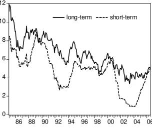
In what follows, we estimate an equation for yields of 10Y US Treasuries from the mid 1980s

until mid-2006. Thus, we concentrate mainly on the Greenspan era. On the right hand side, we

distinguish between long-run influences and determinants of short-run dynamics. This split is

done by economic reasoning and unit root tests. The short-term interest rate is the 3-month

money market rate. Both interest rates are end-of-month data. End-of-month data have the

advantage of incorporating all information of the respective month and, in contrast to monthly

averages, do not introduce smoothness into the data which in turn leads to autocorrelation in

the residuals (Gujarati, 1995, 405). The two interest rates are shown in figure 1.

0 2 4 6 8 10 12

86 88 90 92 94 96 98 00 02 04 06

long-term short-term

We measure inflation expectations with core inflation, i.e. the annual change of headline CPI

excluding food and energy prices to capture the underlying price trend (see figure 2).4 As a

measure for the state of the business cycle, we use the Institute for Supply Management’s

manufacturing index (ism, see figure 3). It has the advantage (and this is especially important

for forecasting exercises) of not being revised and of being available with only a short

publication lag.

Figure 2: Core inflation

4

1 2 3 4 5 6

86 88 90 92 94 96 98 00 02 04 06

Core Inflation

Figure 3: ISM index

35 40 45 50 55 60 65

86 88 90 92 94 96 98 00 02 04 06

ISM

Our “d”-variable captures structural factors.5 As mentioned above, higher foreign demand for

US Treasuries, due to (i) demand from Asian central banks, (ii) the recycling of petrodollars,

(iii) the strong interest of institutional investors and (iv) liquidity-driven demand due to

world-wide expansionary monetary policies, could be responsible for the low level of US

5

bond yields during the last two years. To quantify the influence of these factors, we include

official and private foreign holdings of US Treasuries ("Treasury Securities") in percent of the

overall federal debt ("total liabilities").6 The following figure 4 shows that, since the

beginning of the Japanese FX market intervention in 2002, the external debt of the US in the

form of Treasuries has increased considerably. Overall, the volume of Treasuries held by

foreigners nearly doubled between 2002 and 2006 from USD 1,100 bn to USD 2,000 bn. This

is equivalent to about 35% of Federal Government`s total liabilities.

Figure 4: Foreign holdings of US Treasuries in % of federal debt outstanding

10 15 20 25 30 35

86 8 8 90 92 94 96 98 00 02 04 06 08

D ebt Ratio

Our sample of monthly data runs from 1986:1 to 2006:6. All variables, except interest rates,

the inflation rate and the foreign debt ratio, are in logarithms. The difference operator Δ refers

to first (monthly) differences.7

3.2 Econometric analysis

Standard unit root tests suggest that most of our variables are I(1) in levels and stationary in

first differences.8 The only exception is the "ism" index which (in line with theoretical

6

Wu (2005) shows that it is not convincing to only concentrate on increases in purchases of US Treasury securities by foreign central banks.

7

All data are available upon request and can alternatively be downloaded at http://freenet-homepage.de/clostermann/data_us_bonds.xls.

8

considerations) is identified as a stationary variable. Owing to the non-stationarity of the time

series, the nominal long-term yield is estimated within a vector error correction model

(VECM) based on the procedure developed by Johansen (1995; 2000). This approach seems to

be particularly suited to verify the long-term equilibrium (cointegration) relationships on

which the theoretical considerations are based. The empirical analysis starts with an

unrestricted VECM which takes the following form:

(5)

1

1 1

−

− − =

Δ = Π_{t t} +

∑

y y y x η ε_t,

where yt represents the vector of the non-stationary variables il, is, πe and d. ε denotes the

vector of the independently and identically distributed residuals, Ψis the coefficient matrix of

exogenous variables and η the vector of constants. The number of cointegration relationships

corresponds to the rank of the matrix Π. Granger’s representation theorem asserts that if the

coefficient matrix Π has reduced rank r < n, then there exist (nxr) matrices α (the loading

coefficients or adjustment parameters) and ß (the cointegrating vectors) each with rank r

(number of cointegration relations) such that Π = αß’ and ß’yt is I(0). The cointegration

vectors represent the long-term equilibrium relationships of the system. The loading

coefficients denote the importance of these cointegration relationships in the individual

equations and the speed of adjustment following deviations from long-term equilibrium. The

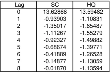
lag order (k) of the system is determined by estimating an unrestricted VAR model in levels

and using the information criteria suggested by Schwarz (SC) and Hannan-Quinn (HQ). All

criteria recommend a lag length of 2 (see table 1).

Table 1: Lag length tests

Lag SC HQ 0 13.62868 13.59482 1 -0.93903 -1.10831 2 -1.35017 -1.65487 3 -1.11267 -1.55279 4 -0.92327 -1.49882 5 -0.68674 -1.39771 6 -0.41889 -1.26528 7 -0.14877 -1.13059 8 -0.01870 -1.13594

The number of cointegration vectors is verified by determining the cointegration rank with the

trace-test and the max-eigenvalue-test. Both tests suggest one cointegration relationship, i.e.

Table 2: Test for the number of cointegration relationships in the VECM

Unrestricted Cointegration Rank Test (Trace) Hypothesized Trace

No. of CE(s) Eigenvalue Statistic Critical Value Prob.** None * 0.1358 55.1177 47.8561 0.0090 At most 1 0.0522 18.0517 29.7971 0.5622 At most 2 0.0171 4.4279 15.4947 0.8661 At most 3 0.0002 0.0443 3.8415 0.8332

Trace test indicates 1 cointegrating eqn(s) at the 0.05 level * denotes rejection of the hypothesis at the 0.05 level **MacKinnon-Haug-Michelis (1999) p-values

Unrestricted Cointegration Rank Test (Maximum Eigenvalue) Hypothesized Max-Eigen

No. of CE(s) Eigenvalue Statistic Critical Value Prob.** None * 0.1358 37.0659 27.5843 0.0023 At most 1 0.0522 13.6238 21.1316 0.3966 At most 2 0.0171 4.3836 14.2646 0.8168 At most 3 0.0002 0.0443 3.8415 0.8332

Max-eigenvalue test indicates 1 cointegrating eqn(s) at the 0.05 level * denotes rejection of the hypothesis at the 0.05 level

**MacKinnon-Haug-Michelis (1999) p-values

Therefore, it seems reasonable to restrict the VECM to one cointegration relationship and, as

the above mentioned unit root tests suggest, to include the indicator for the expected stance of

the business cycle "ism" as a stationary (non-modeled exogenous) variable (with a lag length

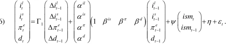
of 0 to 1) into the system. Hence, a VECM with the following structure is estimated:

(6)

(

)

1 1 1 1 1 1 1 1 1 1 − − − − − − − −

⎛ ⎞ ⎛ Δ ⎞ ⎛ ⎞ ⎛ ⎞

⎜ ⎟ ⎜ _Δ ⎟ ⎜ ⎟ ⎜ ⎟ _{⎛ ⎞}

⎜ ⎟_{= Γ} ⎜ ⎟₊⎜ ⎟ ⎜ ⎟_{+ ⎜ ⎟+ +}

⎜ ⎟ ⎜_Δ ⎟ ⎜ ⎟ ⎜ ⎟ _{⎝ ⎠}

⎜ ⎟ ⎜ ⎟ ⎜_⎜ ⎟_⎟ ⎜ ⎟

⎜ ⎟ ⎜_Δ ⎟ _{⎝ ⎠} ⎜ ⎟

⎝ ⎠ ⎝ ⎠ ⎝ ⎠

l l il l

t t t

s s is s

is d

t t t t

t

e e e

t t t t

d

t t t

i i i

i i i ism

ism

d d d

π π α α 1 −

β β β ψ η

π π α π

α

ε .

The long run relationship of this system – after the cointegration coefficients have been

normalized to the long-term interest rate il – is obtained from (il −βis⋅ −is β ππ⋅ e−βd⋅d), where the βs reflect the long-term coefficients.

To interpret the long-term relationship as an equation for the long-term interest rate, however,

all variables except the long-term interest rate il have to be weakly exogenous, i.e. deviations

from the long-term equilibrium are corrected solely through movements of il. As mentioned

above, the extent to which the individual variables adjust to the long-term equilibrium is

captured by the α-values. In a formal test, the null of weak exogeneity of is, d and πe

p-value = 0.60).9 In contrast, the null of weak exogeneity of il has to be rejected at all levels of

significance (χ²(1)= 21.41, p-value = 0.00). Summing up, the following regression results for

the VECM ensue (see table 3). For reasons to be mentioned below, the results and their

implications are not discussed here but in the context of equation (8).

Table 3: Coefficients and test statistics of the VECM (t-values in brackets)

Cointegrating Eq: CointEq il-1 1.00000

is-1 -0.34096

[-5.35907]

πe

-1 -0.54466

[-3.27147] d_-1 0.08133

[ 3.64565] Constant -4.87872

Error Correction: Δil Δis Δπe Δd

α -0.19123 0.00000 0.00000 0.00000 [-6.06881] [ NA] [ NA] [ NA]

Δil_-1 0.15323 0.08281 -0.01582 0.01699 [ 2.36096] [ 1.62024] [-0.49044] [ 0.45743]

Δis-1 -0.18083 0.03621 0.00656 -0.11276

[-2.02968] [ 0.51606] [ 0.14809] [-2.21123]

Δπe

-1 0.09165 -0.05428 -0.02915 -0.13977

[ 0.71014] [-0.53407] [-0.45440] [-1.89215]

Δd-1 0.08131 0.02928 0.00029 0.71839

[ 1.06432] [ 0.48670] [ 0.00769] [ 16.4290] Constant -1.22078 -1.09858 -0.15435 -0.17138

[-4.79346] [-5.47767] [-1.21949] [-1.17570] log(ism) 0.04843 0.02177 -0.00272 -0.01146

[ 5.13196] [ 2.92931] [-0.58086] [-2.12069] log(ism_-1) -0.02567 -0.00100 0.00552 0.01516

[-2.76646] [-0.13728] [ 1.19766] [ 2.85433] R-squared 0.19572 0.20017 0.02051 0.53541 S.E. equation 0.27806 0.21897 0.13819 0.15915 F-statistic 8.55167 8.79494 0.73586 40.50041

Owing to the weak exogeneity of the fundamentals, switching to a single equation error

correction model (SEECM; Engle et al., 1983, Johansen, 1992) may improve the efficiency of

the estimates. We test the existence of a stable long-run relationship within this approach

according to an error correction model, i.e. the significance of the error correction term. To be

more specific, we proceed with the single equation non-linear approach of Stock (1987)

9

When exogeneity is tested for each variable separately the conclusions do not change: is: χ²(1)= 0.39,

where the error correction model and the cointegration relation are estimated

simultaneously.10 Thus, we estimate the following equation:

(7) _{1 1}

1 0 0

( _{− −} ) _{− − −}

= = =

Δ = ⋅l l − ⋅ +

∑

∑

∑

t t t j t j j t j j t j t

j j j

i α i ß z γ i ϕ z ψ x ε

1 − s t i

where z is the vector of I(1)-variables is, d and πe which enter the cointegration space, x is a

vector of (stationary) regressors only entering short-run dynamics (in our case ism), α is the

error correction term and ε is a white-noise residual. The significance of α is assessed

according to the critical values of Banerjee et al. (1998). Significance is taken as evidence of

cointegration.11 To obtain the standard errors and the t-statistics of the long-run coefficients ß,

we estimate the Bewley transformation of the model (West, 1988).

The bracket term of (7) with the variables in levels describes the cointegration relationship

that has been normalized to the long-term interest rate. The lag length (m) is restricted to a

maximum of four. A general-to-specific-modeling is pursued with the so-called backward

procedure, i. e. insignificant coefficients (error probability > 5 %) have been successively

deleted. The final regression reads as (absolute t-values in brackets below coefficients)

(8)

1 1 1 1

(5.8) (6.9) (4.6) (6.9) (2.3)

1 1

(2.4) (4.1) (2.4) (7.1) (2.3)

0.25 ( 0.33 0.56 0.07 8.61)

0.15 1.88 1.02 0.53 0.20

− − − −

− −

Δ = − ⋅ − − + +

+ + − + Δ − Δ

l l s e

t t t t t

l s

t t t t

i i i d

i ism ism i

π

R² = 0.32; SE = 0.25; LM(1) = 0.04; LM(4) = 1.09; ARCH(1) = 0.10; ARCH(4) = 1.10; JB = 1.00; CUSUM: stable; CUSUM square: stable.

The coefficients of the long-run relationship show the theoretically expected signs and are

statistically significant at standard levels. They largely resemble those of the Johansen

procedure. This is indicative of some stability irrespective of the applied econometric

methodology. In the long run, a rise in core inflation has almost a 1-to-1-effect on the

long-term interest rate (assuming that a rise in expected inflation increases the short run interest

rate one to one). This might confirm the existence of the Fisher effect and is in line with

Keeley and Hutchison (1986) who emphasize that this result could be due to monetary regime

stability. The Greenspan era on which we concentrate in this paper obviously was

10

characterized by such stability. The short-term interest rate also exerts a highly significant

positive impact. This result points to the important role of monetary policy and arbitrage in

determining long-term rates. The coefficient on is indicates that a permanent rise in the

short-term interest rate of, say, 100 basis points will result in an increase of the long-short-term interest

rate of 33 basis points.12 Accordingly, the term structure is going to flatten with higher and to

steepen with lower short-term rates (see also Diebold et al., 2006). The less than proportional

response of il to is in the US has also been detected by Ducoudré (2005). The overall impact of

the business cycle, measured by ism, on il is positive, indicating that the effect via the supply

of bonds is dominating (in line with Diebold et al., 2006). The contemporaneous reaction of il

to ism is positive and highly significant. In the short-run, a contemporaneous 1% increase of

the ism results in a 1.9 percentage point increase in il. This value, being greater than 1, implies that the nominal interest rate is on average more volatile than expectations about the future

development of the business cycle. The significantly positive relationship between il and its

first lag may be an indication that the interest rate is in the short run also driven by

non-fundamental factors. This could be due to the market behavior of chartists and technical

analysts (Nagayasu, 1999) whose interest rate forecasts are usually based on past interest rate

movements.

The coefficient of the structural factor d is significantly positive. A value of 0.07 means that

an increase of the debt ratio by 1 percentage point lowers the bond yield by 7 basis points. In

the last four years, the amount of Treasuries held by foreigners increased by about 10

percentage points. This alone would have had a downward impact of 70 basis points on bond

yields. This result is in line with Warnock and Warnock (2005), Frey and Moët (2005) as well

as Bernanke et al. (2004). Longstaff (2004), in contrast, argues that if US investors, who

presumably may benefit more from the highly liquid Treasury market than many foreign

holders of Treasury debt, suddenly begin to purchase Treasuries from these foreign holders,

the yields on Treasuries should increase to reflect the increased popularity of holding

Treasuries. However, he finds that this effect is only significant for maturities up to three

years.

The coefficient of the error correction term is negative and highly significant. Thus, one

condition for long-run stability is satisfied. The parameter estimate of -0.25 suggests a

11

The conclusions of Pesavento (2004) indicate that such kind of tests, if suitably specified, perform better than other cointegration tests in terms of power in large and small samples and are also not worse or better in terms of size distortions.

12

life of shocks of about two months. In other words, the gap between the long-term nominal

interest rate and its equilibrium value is halved within two months after the occurrence of an

exogenous shock. Within one year, the gap is accordingly reduced by over 97%.13

Breusch-Godfrey Lagrange multiplier tests (LM) do not indicate autocorrelation in the

residuals (1st and 4th order). Nor can the Lagrange multiplier (ARCH) test for autoregressive

conditional heteroskedasticity (1st and 4th order) identify any violations of the white-noise

assumptions. In addition, the Jarque-Bera (JB) test confirms the normality of the residuals.

And finally, CUSUM tests do not indicate parameter or variance instability. This once again

underscores the stability of the estimated relation.

In the introduction, we mentioned that some commentators argue that structural or uncommon

factors are needed to explain the recent behavior of bond yields. To examine whether the

foreign debt ratio d captures these structural or uncommon factors adequately, we use the

cointegration relation of our model to calculate a "fair value" of bond yields. Figure 5 shows

that bond markets were overvalued in the course of 2005. But obviously the "disequilibrium"

was not unusually high in a historical perspective. Our four variables seem to capture the

evolution of bond yields quite well. Therefore, it is not necessary to revert to additional

structural or technical factors. In contrast, the macro factors (is, πe, ism) alone are not capable to explain the developments satisfactorily as would have been the case until mid 2005 (see

Clostermann and Seitz, 2005).

13

Figure 5: The fair value of 10-year Treasury bonds (in %)

3 4 5 6 7 8 9 10 11 12

86 88 90 92 94 96 98 00 02 04 06

actual fair value

3.3 Forecast evaluation

In order to assess the quality of our single equation error correction model (SEECM) in

forecasting exercises, we compare it with a random-walk-model (RWM). Following the

influential article of Meese and Rogoff (1983), the RWM has become a very popular

benchmark in forecast evaluation. In line with the unit root tests, the RWM is specified

without a constant or trend.

We run two different kinds of out-of-sample forecasts of up to 12 months into the future. The

first are fully dynamic forecasts which assume that the forecaster has no idea about the future

evolution of the right-hand side variables and bases his predictions of these variables on

simple univariate time series models. Thus, the forecasts include only information that had

actually been available at the time it was carried out. In contrast to this narrow information

set, the second approach assumes that the forecaster knows the true values of the exogenous

variables. Realistically, the actual forecasting environment should be somewhere between

these two extreme cases.

The h-step-ahead forecast error (et+h,t) is calculated as the difference between the actual value

of il at time t+h (ilt+h) and its forecast value (ilt+h,t)

The forecasts are carried out recursively. The “first” estimation period is 1986:1-1995:7 and

the first forecast period runs from 1995:8 to 1996:7. The forecast "window" is then

successively extended month by month. Consequently, the next estimation period is

1986:1-1995:8 and the forecast period is from 1995:9 to 1996:8. And the last forecast period is from

2005:7 to 2006:6. In sum, we get 120 true out-of-sample forecast errors for each "h".

The quality of the forecasts of the competing models is assessed using two criteria. The first is

the root mean squared error (RMSE):

(10) 2 _,

1

1

+ =

=

∑

h t

t h t

RMSE e

T

A smaller RMSE implies better forecast performance. A formal test based on the loss

differential (Diebold and Mariano, 1995) provides information on the significance of the

relative forecasts.

Additionally, we calculate a so-called hit ratio (HR). It assesses the correct sign match and

makes use of an indicator variable J which has the following properties

(

)

(

)

(

)

(

)

l l l l

t h t t h t t

l l l l

t h t t h t t

if sign i i sign i i J if sign i i sign i i J

Therefore, HR is defined as

(11) 1 1 100 = ⎛ ⎞ =_{⎜ ⎟}⋅ ⎝

∑

The higher the HR, the more often the forecast signals the correct direction of interest rate

changes.14 For example, a HR of 70% implies that in 70% of all cases the model predicts the

correct sign of future interest rate changes. The significance relative to the RWM is again

tested according to the test statistics developed in Diebold and Mariano (1995). Both forecast

evaluation criteria - RMSE and HR - are discussed in Cheung et al. (2005).

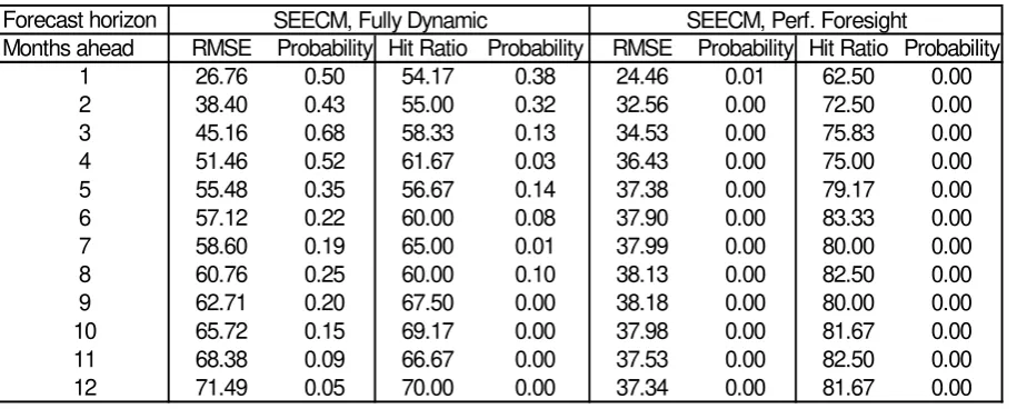
Table 4 shows the two forecasting metrics as well as the p-values of the null that the SEECM

and the RWM have equal forecasting accuracy. As is evident from this table, our model

always outperforms the RWM significantly in the perfect foresight case, i.e. the average

forecast errors of the SEECMs are lower and the signs of interest rate changes are more often

correctly forecasted by the SEECMs. In the fully dynamic case, the predictions of the SEECM

especially true for the RMSE where we are only able to beat the RWM significantly for the

two longest forecast horizons (h=11, 12). Overall, the results underpin the superiority of the

SEECMs, especially for longer forecast horizons. Moreover, it is obvious that the SEECM

does a better job the better the forecaster's predictive abilities with regard to the exogenous

variables.

Table 4: Forecast quality of different models

Forecast horizon

Months ahead RMSE Probability Hit Ratio Probability RMSE Probability Hit Ratio Probability

1 26.76 0.50 54.17 0.38 24.46 0.01 62.50 0.00

2 38.40 0.43 55.00 0.32 32.56 0.00 72.50 0.00

3 45.16 0.68 58.33 0.13 34.53 0.00 75.83 0.00

4 51.46 0.52 61.67 0.03 36.43 0.00 75.00 0.00

5 55.48 0.35 56.67 0.14 37.38 0.00 79.17 0.00

6 57.12 0.22 60.00 0.08 37.90 0.00 83.33 0.00

7 58.60 0.19 65.00 0.01 37.99 0.00 80.00 0.00

8 60.76 0.25 60.00 0.10 38.13 0.00 82.50 0.00

9 62.71 0.20 67.50 0.00 38.18 0.00 80.00 0.00

10 65.72 0.15 69.17 0.00 37.98 0.00 81.67 0.00

11 68.38 0.09 66.67 0.00 37.53 0.00 82.50 0.00

12 71.49 0.05 70.00 0.00 37.34 0.00 81.67 0.00

SEECM, Perf. Foresight SEECM, Fully Dynamic

4. Summary and conclusions

Our results reveal that the development of long-term bond yields in the US can be very well

explained by three standard macroeconomic factors which are widely considered to be the

minimum set of fundamentals needed to capture basic macroeconomic dynamics - monetary

policy, the business cycle and inflation expectations - augmented by the share of Treasuries

held by foreigners.The latter variable captures the structural factors often mentioned in the

literature. These four variables are able to explain the movement of bond yields in a stable

manner. Further macro variables are not needed to capture the evolution of bond yields from

2004 to 2006.

Our forecasting exercises show that we are able to outperform a random walk model. In these

tests, the fully-dynamic approach assumes that the forecaster has no information at all about

the exogenous variables. An assumption that is obviously conservative in real world

applications. On the other side, the perfect foresight case neglects informational deficiencies.

The random walk model which we use as a benchmark might be criticized as being too

"naive" in that it can be improved by including more ar- and ma-terms. Nevertheless, it is

standard in the literature (see, e.g., Cheung et al., 2005). In this respect, one may be interested

14

in further evaluation metrics, e.g. a consistency criterion, to check the robustness of our

results. This is left to future research.

References

Bandholz, H. (2006), US Treasuries: Cyclical Outweighing Structural Factors, HVB Friday Notes, 30 June 2006, 3-5.

Banerjee, A., J. Dolado, D.F. Hendry & G.W. Smith (1986), Exploring Equilibrium Relationships in Econometrics Through Static Models: Some Monte Carlo Evidence,

OxfordBulletin of Economics and Statistics 48, 253-277.

Banerjee, A., J. Dolado & R. Mestre (1998), Error Correction Mechanism Tests for Cointegration in a Single Equation Framework, Journal of Time Series Analysis 19, 267-283.

Bernanke, B.S., V.R. Reinhart & B.P. Sack (2004), Monetary Policy Alternatives at the Zero Bound: an empirical assessment, Finance and Economics Discussion Series of the Federal Reserve Board, 2004-48, September 2004.

Breedon, F., S.G.B. Henry & G.A. Williams (1999), Long-term Real Interest Rates: evidence on the global capital market. Oxford Review of Economic Policy 15, 128–142.

Brooke, M., A. Clare & I. Lekkos (2000), A Comparison of Long Bond Yields in the United Kingdom, the United States and Germany, Bank of England Quarterly Bulletin 40, 150-158.

Campos, J., N. Ericsson & D.F. Hendry (1996), Cointegration Tests in the Presence of Structural Breaks, Journal of Econometrics 70, 187-220.

Caporale, G.M. & G. Williams (2002), Long-term Nominal Interest Rates and Domestic Fundamentals, Review of Financial Economics 11, 119-130.

Cheung, Y.-W., M.D. Chinn & A.G. Pascual (2005), Empirical Exchange Rate Models of the Nineties: Are any fit to survive?, Journal of International Money and Finance 24, 1150-1175.

Christiano, L., M. Eichenbaum & C. Evans (2005), Nominal Rigidities and the Dynamic Effects of a Shock to Monetary Policy, Journal of Political Economy 113, 1-45.

Clostermann, J. & F. Seitz (2005), Are Bond Markets Really Overpriced: The case of the US, University of Applied Sciences Ingolstadt, Working Paper Nr. 11, December.

Demiralp, S. & O. Jordà (2004), The Response of Term Rates to Fed Announcements, Journal of Money, Credit, and Banking 36, 387-405.

Dewachter, H. & M. Lyrio (2006), Macro Factors and the Term Structure of Interest Rates, Journal of Money, Credit, and Banking 38, 119-140.

Diebold, F.X. & R. Mariano (1995), Comparing Predictive Accuracy, Journal of Business and Economic Statistics 13, 253-265.

Diebold, F.X., G.D. Rudebusch & S.B. Aruoba (2006), The Macroeconomy and the Yield Curve: A Dynamic Latent Factor Approach, Journal of Econometrics 131, 309-338.

Durré, A. & P. Giot (2005), An International Analysis of Earnings, Stock Prices and Bond Yields, ECB Working Paper No. 515, August.

Ehrmann, M., M. Fratzscher & R. Rigobon (2005), Stocks, Bonds, Money Markets and Exchange Rates: Measuring International Financial Transmission, NBER Working Paper 11166, March.

Engle, R. & C. Granger (1987), Cointegration and Error Correction: Representation, Estimation, and Testing, Econometrica 35, 251-276.

European Central Bank (2005), Monthly Bulletin April 2005.

European Central Bank (2006), The Accumulation of Foreign Reserves, Occasional Paper No. 43, February.

Fels, J. & M. Pradhan (2006), Fairy Tales of the US Bond Market, Morgan Stanley Research Global, July 26, 2006.

Frey, L. & G. Moët (2005), US Long-term Yields and FOREX Interventions by Foreign Central Banks, Banque de France Bulletin Digest no. 137, May 2005, 19-32.

Greenspan, A. (2005), Testimony Before the Committee on Banking, Housing, and Urban Affairs of the U.S. Senate on February 16, 2005.

Gujarati, D.N. (1995), Basic Econometrics, 3rd ed., McGraw-Hill, Singapore.

Johansen, S. (1995), Likelihood-based Inference in Cointegrated Vector Auto-regressive Models, Oxford University Press, Oxford, New York.

Johansen, S. (2000), Modelling of Cointegration in the Vector Autoregressive Model, Economic Modelling 17, 359-373.

Jordá, O. & K.D. Salyer (2003), The Response of Term Rates to Monetary Policy Uncertainty, Review of Economic Dynamics 6, 941-962.

Keeley, M.C. & M.M. Hutchison (1986), Rational Expectations and the Fisher Effect: implications of monetary regime shifts, Federal Reserve Bank of San Francisco, Working

Papers in Applied Economic Theory86-11.

Kozicki, S. & G. Sellon (2005), Longer-Term Perspectives on the Yield Curve and Monetary Policy, Federal Reserve Bank of Kansas City Economic Review 99, No 4, 5-33.

Longstaff, F.A. (2004), The Flight-to-Liquidity Premium in U.S. Treasury Bond Prices, Journal of Business 77, 511-526.

MacKinnon, J.G., A.A. Haug & L. Michelis (1999), Numerical Distribution Functions of Likelihood Ratio Tests for Cointegration, Journal of Applied Econometrics 14, 563-577.

Meese, R. & K. Rogoff (1983), Empirical Exchange Rate Models of the Seventies: do they fit out of sample?, Journal of International Economics 14, 3-24.

Mehra, Y.P. (1995), Some Key Empirical Determinants of Short-Term Nominal Interest Rates, Federal Reserve Bank of Richmond Economic Quarterly 81/3, 33-51.

Monticini, A. & G. Vaciago (2005), Are Europe's Interest Rates led by Fed Announcements, Working Paper, University of Exeter.

Nagayasu Y. (1999), Japanese Effective Exchange Rates and Determinants: A Long-Run Perspective, in: R. MacDonald & J. Stein: Equilibrium Exchange Rates, Norwell, MA., 323-347.

Pesavento, E. (2004), Analytical Evaluation of the Power of Tests for the Absence of Cointegration, Journal of Econometrics 122, 349-384.

Poole, W. (2005), Understanding the Term Structure of Interest Rates, Federal Reserve Bank of St. Louis Review 87, 589-595.

Rudebusch, G.D., E.T. Swanson & T. Wu (2006), The Bond Yield “Conundrum” from a Macro-Finance Perspective, Federal Reserve Bank of Dallas, Working Paper 2006-16.

Stock, J.H. (1987), Asymptotic Properties of Least Squares Estimators of Cointegrating Vectors, Econometrica 55, 1035-1056.

Tanzi, V. (1976), Inflation, Indexation and Interest Income Taxation, Banca Nazionale del Lavoro Quarterly Review 29, 54-76.

Tobin, J. (1965), Money and Economic Growth. Econometrica 33, 671–684.

Warnock, F.E. & V.C. Warnock (2005), International Capital Flows and U.S. Interest Rates, International Finance Discussion paper 840, September 2005.

West. K.D. (1988), Asymptotic Normality, When Regressors have a Unit Root, Econometrica 56, 1397-1417.

Bisher erschienene Weidener Diskussionspapiere:

1 "Warum gehen die Leute in die Fußballstadien? Eine empirische Analyse der Fußball-Bundesliga" von Horst Rottmann und Franz Seitz

2 "Explaining the US Bond Yield Conundrum" von Harm Bandholz, Jörg Clostermann