Development of Interest in Science and Interest in Teaching Elementary Science: Influence of Informal, School, and Inquiry Methods Course Experiences

ScholarWorks @ Georgia State University

ScholarWorks @ Georgia State University

Mathematics Theses Department of Mathematics and Statistics

5-3-2007

Analyzing the Behavior of Rats by Repeated Measurements

Analyzing the Behavior of Rats by Repeated Measurements

Follow this and additional works at: https://scholarworks.gsu.edu/math_theses

Part of the Mathematics Commons

Recommended Citation Recommended Citation

Hall, Kenita A., "Analyzing the Behavior of Rats by Repeated Measurements." Thesis, Georgia State University, 2007.

https://scholarworks.gsu.edu/math_theses/28

ANALYZING THE BEHAVIOR OF RATS BY REPEATED MEASUREMENTS

by

KENITA A. HALL

Under the direction of Yichuan Zhao

ABSTRACT

Longitudinal data, which is also known as repeated measures, has grown

increasingly within the past years because of its ability to monitor change both within and

between subjects. Statisticians in many fields of study have chosen this way of collecting

data because it is cost effective and it minimizes the number of subjects required to

produce a meaningful outcome. This thesis will explore the world of longitudinal studies

to gain a thorough understanding of why this type of collecting data has grown so rapidly.

This study will also describe several methods to analyze repeated measures using data

collected on the behavior of both adolescent and adult rats. The question of interest is to

see if there is a change in the mean response over time and if the covariates (age,

bodyweight, gender, and time) influence those changes. After much testing, our data set

has a positive nonlinear change in the mean response over time within the age and gender

groups. Using a model that included random effects proved to be a better method than

models that did not use any random effects. Taking the log of the response variable and

using day as the random effect was overall a better fit for our dataset. The transformed

model also showed all covariates except for age as being significant.

ANALYZING THE BEHAVIOR OF RATS BY REPEATED MEASUREMENTS

by

KENITA A. HALL

A Thesis Submitted in Partial Fulfillment of the Requirements for the Degree of

Master of Science

in the College of Arts and Sciences

Georgia State University.

Copyright by

Kenita A. Hall

ANALYZING THE BEHAVIOR OF RATS BY REPEATED MEASUREMENTS

by

KENITA A. HALL

Major Professor: Dr. Yichuan Zhao Committee: Dr. Yu-Sheng Hsu

Dr. Kyle Frantz

Dr. Jun Han

Electronic Version Approval:

ACKNOWLEDGEMENT

Firstly, I would like to thank God for allowing me the opportunity to go back to

school to further my education, which has enhanced me in so many ways.

I must give thanks to my advisor Dr. Zhao. It has been a pleasure to work with

him these past two years. Without his patience and guidance this thesis would not have

been possible.

I would also like to acknowledge my committee members for reviewing my thesis

and providing me with valuable comments. Dr. Frantz, thank you for providing me with

the data set; it was very enlightening and I enjoyed working with you as well.

I want to acknowledge my mother and grandmother for their love and support and

for their assistance with my children while I was in class.

TABLE OF CONTENTS

ACKNOWLEDGEMENT iv

List of Tables vi

List of Figures vii

Chapter One: REPEATED MEASURES 1

1.1 Introduction 1

1.2 Example 2

1.3 Residual Examination 11

Chapter Two: LONGITUDINAL DATA 14

2.1 Objective 14

2.2 Notation 15

2.3 Covariance Structures 15

2.4 Advantages and Disadvantages 18

Chapter Three: UNIVARIATE ANALYSIS OF REPEATED MEASURES 19

Chapter Four: MIXED EFFECT MODELS 26

CHAPTER FIVE: CONCLUSION 47

References 52

List of Tables

Table 3.1: Results from the univariate repeated measures ANOVA 22

Table 3.2: Univariate ANOVA with the test of Sphericity 24

Table 4.1: Results for the standard two way mixed model 27

Table 4.2: Results from the randomly varying intercept model 30

Table 4.3: Results from the random intercept and slope model 32

Table 4.4: Fit Statistic Results 33

Table 4.5: Using the variance component structure 34

Table 4.6: The unstructured structure results 35

Table 4.7: Fit Statistics for the Box-Cox method 38

Table 4.8: Results for the log of the behavior variable 39

Table 4.9: Results for the polynomial transformation 44

List of Figures

Figure 1.1: Time plot of behavior against day 6

Figure 1.2: Mean behavior for age groups at each occasion 7

Figure 1.3: Mean behavior for gender groups at each occasion 8

Figure 1.4: Mean behavior for adults by gender over time 8

Figure 1.5: Mean behavior for periadolescents by gender over time 9

Figure 1.6: Mean behavior for females by age over time 9

Figure 1.7: Mean behavior for males by age over time 10

Figure 1.8: Studentized residuals for behavior 12

Figure 3.1: Individual behaviors against time 20

Figure 4.1 Predicted values of the response as a function of day 40

Figure 4.2: Residuals for transformed response variable 41

Figure 4.3: Scatter plot of behavior versus day (polynomial transformation) 42

Figure 4.4: Predicted values of the response as a function of day 43

Chapter One: REPEATED MEASURES

1.1 Introduction

Longitudinal studies sometimes known as repeated measures are used in many

fields of study and the need to analyze this unique data is growing increasingly.

Sometimes a distinction is drawn between longitudinal designs (where subjects are

followed for extended periods of time) and repeated measures designs (where the

measurements are collected over a relatively short period) (Ware, 1985). This thesis is

focused on explaining longitudinal studies and finding the best model to analyze the data.

Longitudinal data is the union of cross-sectional and time series data. As with many

regression data sets longitudinal data measures a cross section of subjects but unlike most

regression data sets longitudinal data observes the subjects repeatedly over time. Unlike

time-series data, many subjects are observed and the number of measurements per subject

is usually not large in longitudinal studies, (Frees, 2004). Studies that contain data on

individuals who were measured repeatedly over time are defined as longitudinal studies.

(Fitzmaurice, Laird, and Ware, 2004) and (Lindsey, 1999) provide excellent

overviews as well as general theoretical developments and examples of longitudinal data.

Longitudinal data is used to study the changing patterns of the response variable and the

factors that influence those changes both within and between individuals. Within subject

effects are values that differ from measurement to measurement such as time and can

only be achieved within a longitudinal study. Between subject effects are those values

that change only from subject to subject and remain the same for all observations on a

One unique feature of longitudinal data is that they are clustered. The clusters

contain repeated measurements obtained from a single individual at different occasions.

The observations within a cluster will usually display a positive correlation and must be

accounted for in the analysis, which means models used to analyze clustered data must

account for and describe their correlation. Measurements on subjects within a cluster are

more alike than measurements on subjects in different clusters. This assumption

eliminates the assumption of independence that plagues the statistical world.

Repeated measures are a subset of longitudinal designs. The example used in this

thesis consists of repeated measurements that will be analyzed using models that are

appropriate for repeated observations.

1.2 Example

The data used in this thesis is from Mahin Shahbazi’s paper “Age and Sex

Differences in the Acquisition and Maintenance of Intravenous Amphetamine

Self-Administration in Rats”.

The purpose of the study was to investigate differences in vulnerability to

psycho-stimulant drugs such as amphetamine, cocaine or nicotine in adolescent

vs. adult animal (this paper used amphetamine). An operant conditioning

paradigm in which lever pressing behavior is maintained by i.v. drug delivery is

used to create an animal model of human intake.

Operant conditioning is a procedure in which a specific behavior is

enhanced through the process of reinforcement. The subject’s behavior

determines whether or not a reinforcer will be given. A reinforcer or reward is

subject will repeat a behavior if its consequences are rewarding. There are two

parts to operant conditioning: the behavior (something the subject does) and the

consequence (something that happens as a result of the behavior). In the i.v. drug

self-administration example, lever pressing is the behavior and drug infusion is

the consequence. If the behavior (lever pressing) increases when followed by the

consequence (drug infusion) then drug infusion is considered a reinforcer.

Different schedules of reinforcement determines how much lever pressing

behavior is required to receive a reinforcer and under what timetable. There are

two common reinforcement schedules: fixed ratio (FR) and progressive ratio.

Shahbazi’s paper uses both but for the longitudinal study we will only focus on

the fixed ratio. A reinforcement schedule is a rule that states under what

conditions a reinforcer will be delivered. When a reinforcer follows every targeted

response, the schedule is called a continuous reinforcement of fixed ratio 1 (FR1).

The rule for a FR schedule is that a reinforcer is delivered after every n response,

where n is the size of the ratio. Therefore, on a FR10 schedule there is a reinforcer

after every 10 responses.

The rate of acquisition of intravenous amphetamine through

self-administration was compared between periadolescents (ages 35-52 days) and

adults (ages 89-106 days) male and female Spraque Dawley rats. The rats were

housed in groups of 2-3 and placed in chambers and allowed to press between

two levers, an active and an inactive that extended into the chambers at the start of

each session. Pressing the active lever allowed the drug to be pumped from a

consequence but was used to determine whether or not the rats were able to

discriminate between the two levers. Sessions were two hours in duration and

repeated daily for 14 days. Sessions began when the two levers were extended

into the chambers. Lever pressing was reinforced by i.v. injection of

.05mg/kg/0.1ml amphetamine under a FR1, time-out (TO20) schedule. A time-out

(TO20) schedule is where there was a 20 second pause after each infusion (an

infusion was not allowed even if the rat pressed on the active lever). The

concentration of the amphetamine solution was titrated daily to adjust for weight

change.

Behavior (lever pressing) was measured over 14 days to determine if age, sex, and

bodyweight (measured in grams) were factors in the changes of behavior over time. The

random samples consisted of 39 rats (n=8 periadolescent male, n=7 adult male, n=12

periadolescent female, and n=12 adult female) with 14 observations each, for a total of

546 observations. The mean behaviors were 92.46 (male periadolescent), 58.24 (male

adult), 73.84 (female periadolescent), and 62.78 (female adult).The mean body weights

were 210.6 (male periadolescent), 406.9 (male adult), 166.7 (female periadolescent), and

257.9 (female adult). A graphical display of the behaviors at each occasion for each rat is

shown in Figure 1.1

From the graph it can be seen that there is substantial within subject (the jagged

appearance of the line segments) and between subject variability (some rats remain high

throughout the study while others remain low). The graph also shows a slight increase in

A simple t-test was done to determine if there was any difference between the age

and gender groups. For the age group day 3 was chosen to be the time period for the first

t-test. On day 3 nA =19, x=46.08,σ =21.11, and 445.63 2

=

σ for the adults and for

the periadolescentsn_P =20, x=47.75, σ =36.91, and σ2 =1362.35which gave a t

value of .172 which is very small and shows that there is probably no difference in age

groups. Day 8 was also chosen to test for any differences within the age groups. On day 8

19

=

A

n , x=72.32, σ =37.02, and σ2 =1370.48for the adults and n_P =20, x=104.7,

87 . 57

=

σ , σ2 =3348.93for the periadolescents which resulted in a t value of 2.07. This

value is much larger than day 3 and indicates that there maybe some differences in the

age groups as the study progress. For the gender groups’ day 4, day 7, and day 12 were

chosen. On day 4 n_m =15, x=48.5, σ =30.08, and σ2 =904.81for the males and

24

=

F

n , x =54, σ =28.8, and σ2 =829.44for the females which gave a t value of

.188. The hypothesis that the genders are similar would not be rejected because of this

small t value. Day 7 has nm =15, x=103.9, σ =80.5, and 6480.3

2

=

σ for the males

and nF =24, x =64, σ =31.5, and 992.3

2

σ for the females with a t value of 2.12. The

larger t value indicates that there is a difference in the genders response on day 7.

On day 12 the mean response for the males was 90.9 with a standard deviation of

54.2. The females had a mean response of 80.02 and a standard deviation of 28.1. The t

behavi or

0 100 200 300

day

1 2 3 4 5 6 7 8 9 10 11 12 13 14

Figure 1.1 Time plot of behavior against day the genders’ response as the study progressed. Overall there is probably no difference in

the mean response over time within the gender groups.

Time plots for repeated measures on the same subject can be very enlightening.

Time plots are able to show if there are any extreme outliers in the data set and if the

variability in the data changes over time. A plot of the mean response can be very useful

and provides a good basis to selecting a suitable model for the data set. Figure 1.2

displays a plot of the mean behavior at each day for each age group.

Measuring differences in the mean response over time is like measuring the

within individual change (Fitzmaurice, Laird, and Ware, 2004). From Figure 1.2, it can

be seen that the periadolescents mean behavior grew much faster than the adults. The

day 8. The graph also shows some within individual effects. Figure 1.2 agrees with the

t-test that was done earlier. Figure 1.3 shows a plot of the mean behavior at each day for

each gender. From the graph, at the beginning of the study it can be seen that both the

males and females are very similar up to day 3 and then after day 3 the males’ behavior

grew at a much faster rate (the males’ behavior increased by 54% from day 4 to day 5)

than the females until day 11 where their behaviors were almost equal.

age A P

m

20 30 40 50 60 70 80 90 100 110

day

1 2 3 4 5 6 7 8 9 10 11 12 13 14

gender F M m

20 30 40 50 60 70 80 90 100 110

day

1 2 3 4 5 6 7 8 9 10 11 12 13 14

Figure 1.3 Mean behaviors for gender groups at each occasion

age=A

gender F M

m

30 40 50 60 70 80

day

1 2 3 4 5 6 7 8 9 10 11 12 13 14

age=P

gender F M

m

10 20 30 40 50 60 70 80 90 100 110 120 130 140 150

day

1 2 3 4 5 6 7 8 9 10 11 12 13 14

Figure 1.5 Mean behaviors for periadolescents at each occasion

gender =F

age A P

m

20 30 40 50 60 70 80 90 100

day

1 2 3 4 5 6 7 8 9 10 11 12 13 14

gender =M

age A P

m

10 20 30 40 50 60 70 80 90 100 110 120 130 140 150

day

1 2 3 4 5 6 7 8 9 10 11 12 13 14

Figure 1.7 Mean behaviors for males at each occasion

Figure 1.4 and Figure 1.5 are plots of the mean response for each gender by age group.

For the adults near the beginning of the study the males’ behavior increased at a faster

rate than the females until day 8. The females mean response increased by 35% from day

7 to day 8 and continued to maintain a higher mean response rate over the males

throughout the duration of the study.

For the periadolescent rats the males increased by 95% from day 4 to day 5 and

maintained a higher rate over females throughout the duration of the study. The graphs

also show within individual changes as well. The mean response by day for each age

group by gender is also plotted in Figure 1.6 and Figure 1.7. The graphs also show some

within and between subject effects. Both graphs show that regardless of gender the

periadolescents mean behavior starts to increase at a faster rate around day four and

1.3 Residual Examination

Residual analysis also plays an important part in the analysis of longitudinal data.

Residuals can be used to assess the adequacy of the fitted model and can also indicate the

presence of outliers (Fitzmaurice, Laird, Ware, 2004). A scatter plot of the residuals

against the predicted mean response can show if there are any systematic trends. A

residual plot without trends is good and the normal assumptions i) the random errors have

constant variance and ii) the random errors have zero mean are satisfied.

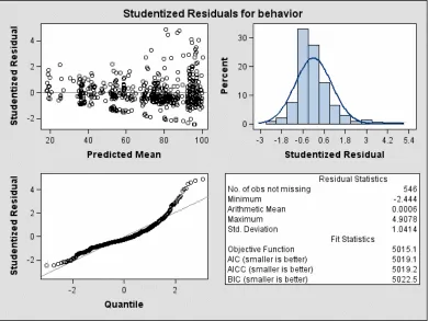
Figure 1.8 has a graphical display of the studentized residuals, the quantile plot,

normal histogram, and the residual statistics for the behavior. From the residual plot, it

can be seen that most of the residuals are scattered around zero but there also appears to

be a slight trend upward and downward at the predicted mean of about 50. The random

variation of the residuals is increasing as the fitted value increases, which is an indication

Figure 1.8 Studentized residuals for behavior

constant. The normal histogram is slightly skewed to the right and the Q-Q plot shows a

plot of the residuals in sorted order against the value the residuals should have if the

distribution of the residuals were normal. The slight curvature in the plot may indicate

that the errors are not from a normal distribution or the data has some outliers. This could

also be due largely to the fact that the observations from the same subject are not

independent and the variance is not constant (correlation exists). It can be concluded that

a distribution other than a normal distribution may be a good model for this data set.

The organization of this thesis is as follows; Chapter 2 will provide the goals of

longitudinal studies and its notation. The different types of covariance structures will also

exploratory analysis and using the univariate repeated measures ANOVA. Chapter 4

reviews the linear mixed effect model and the advantages and disadvantages of using the

model. Chapter 5 contains the conclusion of this thesis and will provide

recommendations for future work. The code used to analyze the data set is listed in the

Chapter Two: LONGITUDINAL DATA

2.1 Objective

Longitudinal data is used to study the pattern of change and the factors that

influence those changes both within and between subjects. Subjects could be individuals,

animals, and or plants that act as their own controls. Longitudinal data requires special

statistical methods because the set of observations on one subject tend to be

inter-correlated. This inter-correlation must be accounted to make a valid inference. Another

goal is to investigate the effects of important covariates on the patterns of change.

There are two types of patterns: Non-time varying covariates, which could be,

gender or age and are considered between (fixed) effects. Time varying covariates such

as weight, time or income are considered within (random) effects (Pahwa and Blair,

2002). Measuring the mean response µ_it =E(Y_it)and seeing how it changes over time

will be the primary goal and the secondary goal will be to draw conclusions about the

parameters that summarize the characteristics of the covariance or correlation among the

repeated measures.

From the above equation, the mean response is allowed to vary over time (which

can be seen by its dependence on the subscript t) and changes in the mean response can

be related to the individual levels of covariates because of its dependence on the subscript

2.2 Notation

Let Y_itbe the response for the ith subject (i=1,...,N) at the tth occasion where

) ,..., 1

(t = ni . The total number of subjects is equal to

∑

N

i i

n , yi =ni×1 is the vector of

responses, and x_it = p×1is the covariate vector for subject i at time t. The matrix of

covariates is X_i =n_i×pfor subject i and will usually include an intercept. For the data

used in this paper i=subject, t=1,...,14, yi =14×1, xit =4×1, and Xi =14×4, the

fixed effects are age and gender because they do not change throughout the duration of

the study and the within individual effects are time and body weight. The data set is also

balanced with time meaning all subjects were measured at a common set of occasions and

there are no missing data.

2.3 Covariance Structures

Although modeling the correlation structure is not of primary importance

it is still however necessary to take into consideration any correlation that may exist when

making statistical inference about longitudinal data. Correlation among subjects will

probably come from three sources of variability: a) between subject effects, b) within

subject effects and c) measurement errors (Fitzmaurice, Laird, and Ware, 2004). An

analysis is not valid unless the covariances among the repeated measures are modeled

properly.

There are several structures that can be used in the analysis of correlated

data with the unstructured (UN) being one of the most commonly used structures. The

(there are no assumptions being made about the variance and the covariance). This

structure is not constrained to be nonnegative definite in order to avoid nonlinear

constraints and therefore it must be symmetric and positive definite. The covariance

matrix                 = 2 3 2 1 3 2 3 32 31 2 23 2 2 21 1 13 12 2 1 ) ( n n n n n n n i Y Cov σ σ σ σ σ σ σ σ σ σ σ σ σ σ σ α K M O M M M K K K

states that the variances across individuals

and the correlations are different. This structure is less powerful when there is missing

data and/or when the size of the sample is not large enough to estimate an unstructured

covariance (the data must be large enough to estimate the

2 ) 1 (n+

n

covariance

parameters). Another

popular structure is the compound symmetry (CS)

                = 1 1 1 1 ) ( K M O M M M K K K ρ ρ ρ ρ ρ ρ ρ ρ ρ ρ ρ ρ i Y Cov

where ρ ≥0is the only constraint. This structure states that the correlations between all

pairs of measures are the same and the variance is constant across occasions. The

compound symmetry is very useful when the mean response is dependent on some

combination of population parameters and a single random effect. The biggest

disadvantage is its assumption that the correlations between any pair of measurements are

the same regardless of time and the variance is constant. Typically, consecutive

farther apart. The assumption that the variance is constant is also not valid within

longitudinal studies.

The auto regressive (1) [AR(1)] structure

                = − − − − − − 1 1 1 1 ) ( 3 2 1 3 2 2 1 2 K M O M M M K K K n n n n n n i Y Cov ρ ρ ρ ρ ρ ρ ρ ρ ρ ρ ρ ρ

resolves some of the objections the compound

symmetry has with successive data and when the measures are equally spaced over time.

The AR(1) structures states that the variance is constant and the correlations between two

responses that are t measurements apart are ρt where ρ ≥0. With this structure, the

correlations decrease over time, which is assumed to happen in longitudinal data but most

longitudinal studies will not decrease as fast. This structure is only appropriate when the

measurements are made at equal time intervals.

The Toeplitz TOEP covariance structure

                = − − − − 2 2 1 2 2 1 2 1 1 2 2 1 2 1 ) ( σ σ σ σ σ σ σ σ σ σ σ σ σ σ σ σ K M O M M M K K K n n n n n n i Y Cov

assumes pair of responses that are equally spaced in time have the same correlation and

the variance does not have to be constant. This structure is also only valid when the

measurements are taken at the same time intervals.

The first order factor analytic without the diagonal matrix D [FA0(q)] can be used

when the structure is nonnegative definite. When the number of random factors is less

be used to approximate the unstructured matrix in the random statement, where q is equal

to the number of random effects.

The variance component VC structure is the default structure for the random and

repeated statements used in the mixed models. When used in the random statement a

separate variance component is assigned to each effect and when used in the repeated

statement, it will specify a heterogeneous variance model. All of the above models can be

used with the constraint that the variance is heterogeneous which is true in most

longitudinal studies. Ignoring the correlation can cause the inferences about the

regression parameters to be incorrect, the estimates of β will be inefficient, and there will

be no protection against biases, which is caused by missing data.

2.4 Advantages and Disadvantages

There are several advantages and disadvantages to using longitudinal studies.

Some of the advantages are: subjects serving as their own controls which mean the direct

study of change can be measured, fewer subjects are required because the measurements

are being repeated, between-subject variation is excluded from the error, and longitudinal

data can separate aging effects from cohort effects. Some of the disadvantages are: the

dependence of the measurements which must be accounted for in the analysis, models are

not as well developed; the risk of attrition, carry-over effects, and the improvement or the

Chapter Three: UNIVARIATE ANALYSIS OF REPEATED

MEASURES

There are three main approaches to analyzing longitudinal data:

Marginal Analysis: where the mean of the response is of importance

Random Effects Models: used to determine how the regression coefficients

change over the individuals

Transitional Models: where its main focus is to determine how the response

variable for a specific subject at time tdepends on past values of the response and

other variables.

Marginal Models focus on the average of the response variable and how that average

changes over time. For the data set used in this thesis using marginal models would

answer the question: Does the average lever pressing behavior change over time and does

age, gender, bodyweight, and time influence those changes?

A simple analysis of longitudinal data is done by the univariate repeated measures

ANOVA. The ANOVA is used to compare and estimate groups in terms of their means

and their trends over time. There are several assumptions that must be met in order to use

the repeated measures ANOVA.

The data and errors are normally distributed

The group comparisons are not used to explain individual growth

There is no missing data

The data must also be balanced

Figure 3.1 Individual behaviors plotted against time

In the univariate repeated measures ANOVA the correlation is assumed to come

from the individual specific random effects; this is due to the fact that each subject is

assumed to have an underlying level of response that persists over time and influences all

measurements on that subject. The times of measurement are treated as a within-subject

factor and the effect of time is assumed to be the same for all subjects. The response for

the ith subject is assumed to be related to discrete covariates and is assumed to be

different from the population meanµ.

Repeated measures ANOVA can be expressed as yij =µ +τi +ν j +eij, where

j ij

ij X Y

E( )= ′ =µ+ν . The parameter νjis the effect of time. The

variance, and e_ij ~N(0,σ_e2)is a within-subject measurement error and it gives the

within-subjects variance. The covariance matrix of the ANOVA has a compound

symmetry structure, where the variance and covariance are homogeneous across time and

equal to στ2 +σe2 and

2

τ

σ , respectively. The correlation between two repeated measures

is therefore equal to _{2 2}

2

e σ σ

σ

τ τ

+ .

The first step in analyzing longitudinal data is to create graphs of the group means

against time (shown in Chapter 1) and the individual responses against time, which are

shown in Figure 3.1. All of the individuals are increasing but not linearly and exhibit

significant within subject effects. Some of the rats exhibit a constant mean response

profile; which means there was no time effect for those subjects.

Secondly, an analysis of the covariance and correlation matrix should be done to

determine what structure is best for the data set. Performing a correlation test on the data

for each gender and age group revealed the covariance matrix for the both gender groups

exhibited heterogeneous variance and covariance. The correlation matrices appear to

have an unstructured structure (where the correlations are all different); or a

heterogeneous Toeplitz structure (where the correlations are the same for a pair of

responses that are equally separated in time). The correlations for the females appear to

be higher than the male correlations. For the age groups, the covariance matrices also

exhibit heterogeneous variance and covariance. The covariance is neither increasing nor

decreasing in a continuous manner. The correlation matrices for both age groups also

resemble a heterogeneous Toeplitz or unstructured structure.

SOURCE DF

SUM OF SQUARES

MEAN SQUARE

F

VALUE Pr > F

Model 40 670608.72 16765.22 17.45 <.0001

Error 505 485211.82 960.82

Corrected

Total 545 1155820.546

Tests of Hypotheses for Mixed Model Analysis of Variance

SOURCE DF Type III SS

MEAN SQUARE

F

VALUE Pr > F

gender 1 1266.85 1266.85 .34 0.5637

Error 57.33 215358 3756.30

Error: 0.2241*MS(rat(gender)) + 0.7759*MS(Error)

rat(gender) 37 497018.35 13432.93 13.98 <.0001

* day 1 157324 157324 163.74 <.0001

gender*day 1 153.59 153.59 .16 .6895

Error:

MS(Error) 505 485212 960.82

* This test assumes that one or more other fixed effects are zero

R

Square Coeff Var Root MSE

Mean

behavior

0.5802 43.55 30.99 71.17

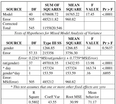
Table 3.1 Results for the univariate repeated measures ANOVA

It can be concluded that a model that uses an unstructured or Toeplitz model may

fit the data best. Using those structures with heterogeneous variance is also recommended

given the design of the covariance matrix.

Table 3.1 shown below gives the results for the dependent variable using the

univariate repeated measures ANOVA by gender. The Type III test shows the gender by

day interaction as being significant at the .05 level. Therefore, the hypothesis that the

groups are the same over time would be rejected (this could also be verified by the graphs

of the mean response in Chapter 1) and it can be concluded that the average mean

response for the gender groups are not the same over time. The fixed effect gender is not

gender is treated as our treatment factor. The r-square value of .6404 validates the

assumption that correlation exists.

One might question these results because the ANOVA assumes that the

covariance matrix has a compound symmetry structure and the variances of the residuals

for each of the time points are the same (Kristensen and Hansen, 2004). Plotting the

residuals at each occasion as box plots is a good way to see if the residuals are constant.

For our study this is not true and the assumption of variance homogeneity has been

violated. From previous results, the covariance matrix for the data used in this thesis

appears to have a Toeplitz or unstructured structure, which means the results of the

ANOVA test, may be invalid because the F ratios may not have an F distribution. Having

an F distribution is dependent on the data having a covariance matrix that is similar to a

compound symmetry structure. To test whether the assumptions of the univariate

repeated measures ANOVA have been violated one can use the sphericity test.

The results from the univariate repeated measures ANOVA that includes the test

of sphericity are shown in Table 3.2. From the results of the sphericity test, the

hypothesis that the structure of the covariance matrix is a compound symmetry would be

rejected. The between- subject variable gender and the within subject effect variable

gender*day are also not significant. The results for the between and within variables are

based on the assumption that the compound symmetry structure of the covariance matrix

Sphericity Tests Variables DF

Mauchly's Criterion

Chi-Square Pr > Chi-Square

Transformed Variates 90 1.15E-07 518.78 <.0001

Orthogonal

Components 90 2.47E-06 419.22 <.0001

Tests of Hypotheses for Between Subject Effects

SOURCE DF

Type III SS

MEAN SQUARE

F

VALUE Pr > F

gender 1 9650.75 9650.75 0.72 0.4021

Error 37 497018.35 13432.93

Univariate Test of Hypothesis for Within Subject Effects G-G F-G

day 13 210431.46 16187.04 18.73 <.0001 <.0001 < .0001

day*gender 13 27065.8 2081.98 2.41 0.0037 .0589 .0498

Error (day) 481 415603 864.04

Table 3.2 Univariate ANOVA with the test of Sphericity

A univariate repeated measures ANOVA test could be done on the age groups but

it is pointless given the fact the covariance matrix for the data set does not exhibit a

compound symmetry structure. The univariate test degrees of freedom is adjusted for data

sets that do not have a compound symmetry structure, this is printed by two different

correction factors. The Greenhouse-Geisser Epsilon (G-G) and the Huynh-Feldt Epsilon

(H-F), which agree with the univariate test by showing day as being significant.

Although, this adjustment exist it is still however not a very good test for our data set

because it does not take into fact that correlation exist, the variance is not constant and

requires the data set to have a normal distribution.

Having a compound symmetry structure, examining only the single aspects of the

subjects and requiring the covariates to be discrete are some of the disadvantages of using

advantages of using the univariate ANOVA would be the fact that the test is easy to do,

Chapter Four: MIXED EFFECT MODELS

Mixed linear models are generalizations of the standard linear model used in the

GLM procedures. It allows data to exhibit correlation and non-constant variance. It also

allows the means to be measured has any other linear model as well as their variances and

covariances. The main assumption of linear mixed effect models is that some subset of

the regression parameters will vary randomly from one subject to another and therefore

accounting for sources of natural heterogeneity in the population (Little, Milliken, Stroup,

and Wolfinger, 1996). SAS PROC MIXED transformed the way repeated measures

analysis is performed. It can handle data that has the univariate or multivariate layout.

PROC MIXED can handle both balanced and unbalanced data. It can also handle missing

data and it applies multiple comparison methods to both the between and within subject

factors (Dallal, 2002). There are three assumptions of the PROC MIXED analysis:

The data is normally distributed

The expected values of the data are linear in trend with respect to certain

parameters

The variances and covariances are in terms of a different set of parameters and

exhibit a structure matching one of those that are available in PROC MIXED

There are two sets of parameters in a mixed linear model that specify the

complete probability distribution of the data. The parameters of the mean model are

referred to as fixed parameters and the variance and covariance parameters are referred to

as the covariance parameters. A distinctive feature of linear mixed models is that the

mean response is modeled as a combination of population characteristics (which are

The population characteristics are called fixed effects and the subject specific effects are

called random effects. Covariance parameters are needed in repeated measurements

because the data exhibits correlation and changing variability.

The statistical model E(Yi)= Xβ is the marginal mean response, which is

averaged over the distribution of random effects. Inclusion of random effects produces

covariances among the responses, states that the Cov(Yi)=Σi has a unique random

effects structure, and it allows the covariances of the repeated measures to be expressed

as functions of time. A linear mixed effect model explicitly distinguishes between within

(random) and between (fixed) subject variability.

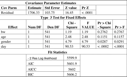
Producing a standard two-way analysis of variance using PROC Mixed produced

the following result:

Covariance Parameter Estimates

Cov Parm Estimate Std Error Z value Pr Z

Residual 1706.33 103.75 16.45 < .0001

Type 3 Test for Fixed Effects Effect Num DF Den DF

Chi -Square

F VALUE

Pr > Chi

- Square Pr > F

bw 1 541 1.19 1.19 0.2762 0.2767

age 1 541 2.48 2.48 0.1151 0.1157

gender 1 541 4.79 4.79 0.0287 0.0291

day 1 541 90.53 90.53 < .0002 <.0001

Fit Statistics

- 2 Res Log likelihood 5599.9

AIC 5601.9

AICC 5602

BIC 5606.2

The “Covariance Parameter Estimates” table gives the estimate σ2for the model and the

“Fitted” table lists information about the restricted/residual likelihood along with other

values that help determine if the model is a good fit or not. The Type III test results show

that gender and day are significant factors in the model at the 5% level.

From the above results, the model does not seem to be a very good fit for this

data. This could be due to the fact this model assumes that the data has a normal

distribution and the observations are independent with constant variance. The normality

assumption is valid because the response values are all real numbers but because the data

is being repeated there is a very high probability that the observations on the same subject

are correlated and therefore not independent. The correlation between the subjects can be

modeled using one of the covariance structures described previously.

One of the simplest ways of modeling correlation is through the use of random

effects. Random effect models for longitudinal studies are regression models in which

the regression coefficients are allowed to vary across the subjects. Random effects set up

a common correlation among all observations having the same level. Random effects not

only allow for the trend over time to be described while taking into account that

correlation exists between consecutive measurements, it also describes the variation in

the baseline measurement and in the rate of change of time. Random effects can be used

to build hierarchical models that correlate measurements made on the same level of a

random factor (Moser, 2004). The standard mixed model equation is listed below:

ε γ β + + = X Z

where X is the matrix of fixed effects, β is the unknown fixed parameters, Z is the

random design matrix and γ is the unknown random parameters (Little, Milliken, Stroup,

and Wolfinger, 1996).

The random statement in the PROC MIXED model defines the random effects for

the γ vector in the model, which can be used to specify the traditional variance

components. The main purpose of the random statement is to define the Z matrix for the

random effects and to define the structure of G matrix, which is the variance – covariance

matrix. The Z matrix is built just like the X matrix for the fixed effects. The model

it i

ij day b

Y =β₁+β₂ + +ε

allows the subject to vary randomly.

This model (randomly varying subject effect) assumes that each subject has an

underlying level of response that continues over time. The variable b_iis the random

subject effect that describes how the trend over time for the ith subject deviates from the

population mean (represents the influence of subject i on its repeated measurements). The

above model describes how the response for the ith subject at the tth time differs from the

population mean 'β

it

X by the subject effect biand the within subject measurement

errorε_it. The subject effect and the measurement error are independent of each other and

are believed to vary randomly with a mean of zero and a variance of Var(bi)=σb2for the

subject effect and Var(ε_ij)=σ2 for measurement error. The model for the randomly

Covariance Parameter Estimates Cov Parm Subject Estimate

Std

Error Z value Pr Z

Intercept rat 883.87 218.53 4.04 < .0001

Residual 959.22 60.31 15.91 < .0001

Type 3 Test for Fixed Effects Effect Num DF Den DF

Chi -Square

F VALUE

Pr > Chi

- Square Pr > F

day 1 506 170.75 170.75 <.0001 <.0001

Solution for Fixed Effects

Effect Estimate Std Error DF t value Pr > |t|

Intercept 38.95 5.52 38 7.05 < .0001

day 4.3 0.329 506 13.07 < .0001

Fit Statistics

- 2 Res Log likelihood 5394.4

AIC 5398.4

AICC 5398.4

BIC 5401.7

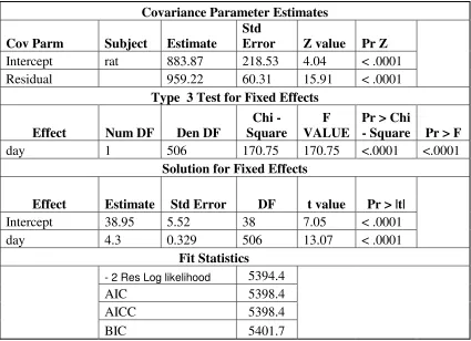
Table 4.2 Results from the randomly varying intercept model

This model used the variance component structure and the restricted maximum

likelihood. The G and GCORR matrix produced the variance/covariance matrix and the

correlation matrix respectively for the first subject. Allowing day to be random produces

an AIC value of 5398.4 and a BIC value of 5401.7, which is much lower than the model

without any random slopes. The type 3 test shows day to be significant at the 5% level.

The F value is used to test H_o :µ₁ =µ₂ =...=µ₁₄ against H_a since the p-value is less

than .05, the null hypothesis would be rejected.

The model

it i

ij day age gender bw b

includes the other fixed effects while still allowing the subjects to vary randomly. The

results give an AIC value of 5377.9 and a BIC value of 5381.3, which is an indication

this is a better fit than the model with day being the only fixed effect. The fixed effects

day, age, and bodyweight are significant at the 5% level. The results also show that the

females’ behavior starts off higher than the males and the starting point for the adults is

also larger than those for the periadolescents.

Next, we will look at a model that allows for both the intercept and slope to vary

randomly.

ij i i ij

ij t b b

Y =β₁+β₂ + ₁ + ₂ +ε

is a linear mixed effects model with randomly varying intercepts and slopes among the

subjects. Each subject varies at the baseline level of response (t_i1 =0 in this case t_i1is

equal to day one) and in changes of their responses over time. The measurement errors

allow the response at any occasion to vary randomly above and below the subject specific

trajectories (Fitzmaurice, Laird, and Ware, 2004). Let’s examine the above mixed effect

model with time being the randomly varying slope and the variance component as the

structure of the G matrix. Allowing for the intercept and the slope to be random proves to

be a better fit than the random subject effect, which is shown by the AIC value of 5341.2

and the BIC value of 5346.2. This model shows that the fixed effect is significant given

the variable time (day) as random.

Now, we will look at the same model with the unstructured covariance, the

autoregression (1), Toeplitz, and compound symmetry structures. Table 4.4 shows the

results of the fit statistics. The model that used the unstructured structure and allowed the

structures (this is determined by the AIC and BIC values). With the unstructured structure

only two iterations were needed to find the maximum likelihood where the restricted

maximum likelihood was used to estimate the regression coefficients. The model with the

compound symmetry needed ten iterations to find the residual/restricted maximum

likelihood.

Table 4.3 Results from the random intercept and slope model Covariance Parameter Estimates

Cov Parm Subject Estimate

Std

Error Z value Pr Z

Intercept rat 667.82 199.58 3.35 0.0004

day rat 9.15 2.74 3.34 0.0004

Residual 779.74 51.35 15.19 < .0001

Type 3 Test for Fixed Effects Effect Num DF Den DF

Chi -Square

F VALUE

Pr > Chi

- Square Pr > F

day 1 38 57.25 57.25 <.0001 <.0001

Solution for Fixed Effects

Effect Estimate Std Error DF t value Pr > |t|

Intercept 38.95 4.84 38 8.04 < .0001

day 4.3 0.568 38 7.57 < .0001

Fit Statistics

- 2 Res Log likelihood 5335.2

AIC 5341.2

AICC 5341.3

BIC 5346.2

Estimated G Matrix

Row Effect rat Col1 Col2

1 Intercept Rat166 667.82

2 day Rat166 9.15

Estimated G Correlation Matrix

Row Effect rat Col1 Col2

1 Intercept Rat166 1

UN AR(1) TOEP CS

- 2 Res Log likelihood 5331.7 5385.8 5385.6 5385.8

AIC 5339.7 5389.8 5391.6 5389.8

AICC 5339.8 5389.8 5391.6 5389.8

BIC 5346.4 5389.8 5396.5 5393.1

Table 4.4 Fit Statistic Results

With a p-value of <.0001, the variable day is significant at the α =.05 level of

significance for the model.

The above models did not include the other covariates age, gender, and

bodyweight. The next model

ij ij i i ij

ij t age gender bw b b t

Y =β₁ +β₂ +β₃ +β₄ +β₅ + ₁ + ₂ +ε

will include the additional covariates and leaving time as the randomly varying slope.

The results for the model that uses the variance component and REML method are given

in Table 4.5. This model has a variance of 780.4 and an AIC and BIC value that are lower

than the previous models. The fixed effect day is the only one that is significant at the

05 .

=

α level.

Analysis of the previous model was done with the unstructured covariance, the

autoregression (1), Toeplitz, and compound symmetry structures. The model that uses the

UN structure fits the data best. The UN, AR(1), CS, and TOEP produced the following

AIC values 5327.6, 5381.3, 5381.3 and 5383.0, respectively. The BIC values were

5334.3, 5384.6, 5384.6 and 5388.0, respectively. The heterogeneous models of the

covariance structures and the FA0(2) structure were also tested and produced the same

AIC value as the unstructured structure. The unstructure structure produced a variance of

Table 4.5 Results from the variance component structure model

produced a variance of 945 and needed nine iterations to maximize the likelihood. In all

of the models, day was the only fixed effect that was significant.

The model ij ij i i ij

ij t age gender bw gender day age day b b t

Y =β₁ +β₂ +β₃ +β₄ +β₅ +β₆( ⋅ )+β₇( ⋅ )+ ₁ + ₂ +ε

will include the gender*day and age*day interaction terms. The interaction terms will

determine if the null hypothesis: “changes among time (day) is the same for the groups”

is true or not. Table 4.6 shows the results for the above model using the unstructured

Covariance Parameter Estimates Cov Parm Subject Estimate

Std

Error Z value Pr Z

Intercept rat 730.39 222.63 3.28 0.0005

day rat 8.74 2.72 3.21 0.0007

Residual 780.44 51.47 15.16 < .0001

Type 3 Test for Fixed Effects Effect

Num

DF Den DF

Chi -Square

F VALUE

Pr > Chi

- Square Pr > F

day 1 38 39.88 39.88 <.0001 <.0001

age 1 467 0.75 0.75 0.386 0.3864

gender 1 467 0 0 0.9936 0.9936

bw 38.95 467 0.76 0.76 0.3845 0.3849

Fit Statistics

- 2 Res Log likelihood 5324.1

AIC 5330.1

AICC 5330.1

BIC 5335.1

Estimated G Matrix

Row Effect rat Col1 Col2

1 Intercept Rat166 730.39

2 day Rat166 8.74

Estimated G Correlation Matrix

Row Effect rat Col1 Col2

1 Intercept Rat166 1

structure. The model was also tested using the Autoregressive (1) and the Toeplitz

structures, which gave AIC values of 5368.7 and 5369.5 and BIC values of 5372.0 and

5374.5 respectively. From the results it is obvious that a model that uses an unstructured

structure fits the data set best. This agrees with our results from Chapter 3.

The results shown in Table 4.6 give the covariance and correlation matrices and

Covariance Parameter Estimates Cov Parm Subject Estimate

Std

Error Z value Pr Z

UN(1,1) rat 863.95 263.03 3.28 0.0005

UN(2,1) rat -36.17 22.12 -1.64 0.102

UN(2,2) rat 8.87 2.9 3.06 0.0011

Residual 771.06 50.42 15.29 < .0001

Test of Fixed Effects Effect

Num

DF Den DF

Chi -Square

F VALUE

Pr > Chi

- Square Pr > F

day 1 36 43.16 43.16 <.0001 <.0001

age 1 467 0.27 0.27 0.61 0.61

gender 1 467 0.48 0.48 0.49 0.49

bw 1 467 0.12 0.12 0.73 0.73

day*gender 1 467 0.03 0.03 0.87 0.87

day*age 1 467 8.56 8.56 0.0034 0.0036

Fit Statistics

- 2 Res Log likelihood 5307.1

AIC 5315.1

AICC 5315.2

BIC 5321.8

Estimated G Matrix

Row Effect rat Col1 Col2

1 Intercept Rat166 863.95 -36.17

2 day Rat166 -36.17 8.87

Estimated G Correlation Matrix

Row Effect rat Col1 Col2

1 Intercept Rat166 1 -0.413

2 day Rat166 -0.413 1

show day and age*day as being significant at the α =.05level. The age*day term will be

discarded because age alone is not significant. The results also show that the null

hypothesis would not be rejected and it can be concluded that the trends in the mean

response over time are the same in the gender groups (because of the short study period

and this is a linear model we can not conclude that there is no difference within the

gender groups). Including the interaction terms in the model reduced the AIC value and

proved to be a better fit than the models used previously at the beginning of the chapter.

The assumption of a linear transformation between y and the regressors is not

always valid. Looking back at the figures in Chapter 1 it can be seen that the response

variable may have a nonlinear over time. A nonlinear function can be linearized by using

a suitable transformation (Montgomery, Peck, and Vining, 2001). A commonly applied

transformation for positive value data is to take the log of the value. The transformed

values will then have a full range (−∞,∞), which allows a method based on normal

distributions to become more reasonable, Crowder and Hand (1990). Taking the log of

the response variable will linearize the above model.

The new intrinsically linear model will be

ij ij i i ij ij t b b day bw day gender day age gender age bw t Y ε β β β β β β β β + + + ⋅ + ⋅ + ⋅ + + + + + = 2 1 8 7 6 5 4 3 2 1 ) ( ) ( ) ( ) ln(

which implies that the multiplicative error term in the original model is log normally

distributed. Taking the log of the response variable is a special case of the Box – Cox

method where λ=0. The parameters of the model and λ can be estimated

simultaneously by the method of maximum likelihood which is explained in Box and

log-transforming the data reduces the overall variability and may help reduce the problem

of variance heterogeneity.

Figure 4.2 shows a graph of the residuals for the transformed response variable.

The fit statistics show that taking the log transformation improved the fit of the model.

Table 4.7 shows that taken the log of the response and analyzing the model with the new

response variable is a much better fit for this data set. The AIC and BIC values dropped

significantly. The AIC values for the Autoregressive (1), Toeplitz, produced AIC values

of 1393.3 and 1322.6 and BIC values of 1396.7 and 1327.5, respectively. These results

confirm the analysis that was done in Chapter 3. The results in Table 4.7 still show day

and the interaction variable (age*day) as the only fixed factors being significant at the .05

level. The p-value for the age*day did however increase from the previous results and is

no longer significant at the α =.01 level. Removing the insignificant term age produced

an AIC value of 1144.7 and a BIC value of 1151.3, which is a slight increase from the

full model.

Other useful power transformations foryλ, are

2 1 2 1 ,

1− and

− =

λ . The fit statistic

results are shown in Table 4.8. The results also show that the log transformation will give

the best fit. Figure 4.1 shows a plot of the predicted values as a function of day. Based on

our results the best model for our data set is

ij ij i i ij

ij t bw gender gender day bw day b b t

Y )= β₁ + β₂ +β₃ + β₄ + β₅( ⋅ )+ β₆( ⋅ )+ ₁ + ₂ +ε

ln(

and the results are listed in Table 4.10. Plots of the final model versus the observed

response values for some of the subjects are shown in Figure 4.5. Figure 4.5 contains a

plot of both the female and male rats from both age groups. The predicted responses also

the test. Within the males the periadolescent rats have a steeper slope, which is an

indication that they (periadolescent males) acquired faster than the adults and maintained

a higher rate throughout the duration of the study. Within the females there does not seem

to be much of a difference between the periadolescent and adult rats. The predicted

values are almost mirror images of each other. This is an indication the means for both

age groups are probably the same or the difference between the two is very small.

-1 2

1

−

0 2

1

- 2 Res Log likelihood -627 -732.2 1132.5 2259.5

AIC -619 -724.2 1140.5 2267.5

AICC -618 -724.1 1140.5 2267.6

BIC -612.3 -717.5 1147.1 2274.1

Covariance Parameter Estimates Cov Parm Subject Estimate

Std

Error Z value Pr Z

UN(1,1) rat 1.54 0.393 3.92 < .0001

UN(2,1) rat -0.107 0.0296 -3.62 0.0003

UN(2,2) rat 0.0085 0.0024 3.54 0.0002

Residual 0.324 0.021 15.09 < .0001

Test of Fixed Effects Effect

Num

DF Den DF

Chi -Square

F VALUE

Pr > Chi

- Square Pr > F

bw 1 460 13.16 13.16 0.0003 0.0003

age 1 460 3.02 3.02 0.0824 0.0831

gender 1 460 5.94 5.94 0.0148 0.0151

day 1 36 47.81 47.81 < .0001 < .0001

day*age 1 460 7.37 7.37 0.0066 0.0069

day*gender 1 460 16.6 0 < .0001 < .0001

day*bw 1 460 30.2 30.2 < .0001 < .0001

Fit Statistics

2 Res Log likelihood 1132.5

AIC 1140.5

AICC 1140.5

BIC 1147.1

Estimated G Matrix

Row Effect rat Col1 Col2

1 Intercept Rat166 1.54 -0.107

2 day Rat166 -0.107 0.0085

Estimated G Correlation Matrix

Row Effect rat Col1 Col2

1 Intercept Rat166 1 -0.9347

2 day Rat166 -0.9347 1

r oot _behavi or = 5. 5388 +0. 3174day

N 546 Rsq 0. 1935 Adj Rsq 0. 1921 RMSE 2. 6166

5. 5 6. 0 6. 5 7. 0 7. 5 8. 0 8. 5 9. 0 9. 5 10. 0

day

0 2 4 6 8 10 12 14

Figure 4.2 Residuals for the transformed response variable

Now, we will do one more transformation to see if it fits the data better and to also verify

how conclusion about taking the log of the response variable. Based on Figure 4.3 and

Figure 4.4 a polynomial transformation may be a good fit the data but we will need to

0 50 100 150 200 250

2 4 6 8 10 12 14

day

b

e

h

a

vi

o

r

Figure 4.3 Scatter plot of behavior versus day (polynomial transformation)

The model for the polynomial transformation is Y_ij =β_o +β day+β day2 +ε_ij

2

1 . In this

model we wish to estimate the intercept, the slope coefficient for the linear day term, and

the slope coefficient for the quadratic day (squared) term. The results listed in Table 4.9

show day and daysq are significant at the α =.05 level but the AIC and BIC values are

much higher than the AIC and BIC values for the Box – Cox method previously done.

Therefore we can conclude our final model (log transformation of the response variable)

behavi or = 16. 592 +12. 681day - 0. 559 daysq

N 546 Rsq 0. 1724 Adj Rsq 0. 1694 RMSE 41. 971

20 30 40 50 60 70 80 90

day

0 2 4 6 8 10 12 14

Figure 4.4 Predicted values of the response as a function of day

Some of the disadvantages of using the Mixed Model are: Date will need to be

continuous and normally distributed and mixed models only model the data as

polynomials. Overall, mixed models are probably the best (linear model) because it

allows the data to have both fixed and random effects, it can handle the assumption of

dependence among the subjects and provides a large variety of useful covariance

Covariance Parameter Estimates Cov Parm Subject Estimate

Std

Error Z value Pr Z

UN(1,1) rat 830.59 241.87 3.43 0.0003

UN(2,1) rat -37.88 22.35 -1.69 0.0901

UN(2,2) rat 11.38 3.32 3.43 0.0003

Residual 695.98 45.55 15.28 < .0001

Type 3 Test of Fixed Effects Effect Num DF Den DF

Chi -Square

F VALUE

Pr > Chi

- Square Pr > F

day 1 38 91.93 91.93 < .0001 <.0001

daysq 1 467 50.98 50.98 < .0001 < .0001

Solution for Fixed Effects

Effect Estimate Std Error DF t value Pr > |t|

Intercept 16.59 6.06 38 2.74 0.0094

day 12.68 1.32 38 9.59 < .0001

daysq -0.559 0.078 467 -7.14 < .0001

Fit Statistics

- 2 Res Log likelihood 5286.2

AIC 5294.5

AICC 5294.6

BIC 5301.1

Estimated G Matrix

Row Effect rat Col1 Col2

1 Intercept Rat166 830.59 -37.88

2 day Rat166 -37.88 11.38

Estimated G Correlation Matrix

Row Effect rat Col1 Col2

1 Intercept Rat166 1 -0.39

2 day Rat166 -0.39 1