Evaluating revised biomass equations: are some forest types more equivalent than others?

(1)

RESEARCH

Evaluating revised biomass equations:

are some forest types more equivalent

than others?

Coeli M. Hoover

*

_{and James E. Smith}

Abstract

Background: In 2014, Chojnacky et al. published a revised set of biomass equations for trees of temperate US forests, expanding on an existing equation set (published in 2003 by Jenkins et al.), both of which were developed from published equations using a meta-analytical approach. Given the similarities in the approach to developing the equa-tions, an examination of similarities or differences in carbon stock estimates generated with both sets of equations benefits investigators using the Jenkins et al. (For Sci 49:12–34, 2003) equations or the software tools into which they are incorporated. We provide a roadmap for applying the newer set to the tree species of the US, present results of equivalence testing for carbon stock estimates, and provide some general guidance on circumstances when equation choice is likely to have an effect on the carbon stock estimate.

Results: Total carbon stocks in live trees, as predicted by the two sets, differed by less than one percent at a national level. Greater differences, sometimes exceeding 10–15 %, were found for individual regions or forest type groups. Dif-ferences varied in magnitude and direction; one equation set did not consistently produce a higher or lower estimate than the other.

Conclusions: Biomass estimates for a few forest type groups are clearly not equivalent between the two equa-tion sets—southern pines, northern spruce-fir, and lower productivity arid western forests—while estimates for the majority of forest type groups are generally equivalent at the scales presented. Overall, the possibility of very differ-ent results between the Chojnacky and Jenkins sets decreases with aggregate summaries of those ‘equivaldiffer-ent’ type groups.

Keywords: Biomass estimation, Allometry, Forest carbon stocks, Tests of equivalence, Individual-tree estimates by species group

© 2016 Hoover and Smith. This article is distributed under the terms of the Creative Commons Attribution 4.0 International License (http://creativecommons.org/licenses/by/4.0/), which permits unrestricted use, distribution, and reproduction in any medium, provided you give appropriate credit to the original author(s) and the source, provide a link to the Creative Commons license, and indicate if changes were made.

Background

Nationally consistent biomass equations can be impor-tant to forest carbon research and reporting activities. In general, the consistency is based on an assumption that allometric relationships within forest species do not vary by region. Essentially, nearly identical trees even in dis-tant locations should have nearly identical carbon mass. In 2003, Jenkins et al. published a set of 10 equations for estimating live tree biomass, developed from exist-ing equations usexist-ing a meta-analytical approach, which

were intended to be applicable over temperate forests of the United States [1]. These equations were developed to support US forest carbon inventory and reporting, and had several key elements: (1) a national scale, so that regional variations in biomass estimates due to the use of local biomass equations was eliminated, (2) the exclu-sion of height as a predictor variable, and (3) in addition to equations to estimate aboveground biomass, a set of component equations allowing the separate estimation of biomass in coarse roots, stem bark, stem wood, and foli-age. Since their introduction, these equations have been incorporated into the Fire and Fuels Extension of the Forest Vegetation Simulator as a calculation option [2],

Open Access

*Correspondence: [email protected]

(2)

utilized in NED-2 [3], and have provided the basis for cal-culating the forest carbon contribution to the US annual greenhouse gas inventories for submission years 2004– 2011 (e.g., see [4]). Researchers in Canada [5, 6] and the US (e.g. [7–9]) have also employed the equations while other investigators have adopted the component ratios to estimate biomass in coarse roots or other components (e.g. [10, 11]).

In 2014, Chojnacky et al. [12] introduced a revised set of generalized biomass equations for estimating above-ground biomass. These equations were developed using the same underlying data compilations and general approaches to developing the individual tree biomass estimates as for Jenkins et al. [1], but with greater differ-entiation among species groups, resulting in a set of 35 generalized equations: 13 for conifers, 18 for hardwoods, and 4 for woodland species. Important distinctions are: the database used to generate the revised equations was updated to include an additional 838 equations that appeared in the literature since the publication of the 2003 work or were not included at that time, taxonomic groupings were employed to account for differences in allometry, and taxa were further subdivided in cases where wood density varied considerably within a taxon. The only component equation revised by Chojnacky et al. [12] was for roots; equations were fitted for fine and coarse roots, in contrast to Jenkins et al. [1] where fine roots were not considered separately.

Based on the similarity of the equation development approach, it is likely that applications using the Jenkins et al. [1] set would have essentially the same basis for employing the revised equations. Since the primary objec-tive of Chojnacky et al. [12] was to present the updated equations and describe the nature of the changes, only a brief discussion of the behavior of the updated equations vs. the Jenkins et al. [1] equation set was included. The authors noted that at a national level results were similar, while differences occurred in some species groups, for example, western pines, spruce/fir types, and woodland species. Given the limited information provided in Cho-jnacky et al. [12] we felt that a more thorough investigation of the differences in carbon stock estimates as generated with both sets of equations was needed.

One potentially practical result from a comparison of the two approaches is to identify where one set effectively substitutes for the other, which then suggests that revis-ing or updatrevis-ing estimates would change little from previ-ous analyses. For this reason we applied equivalence tests to determine the effective difference of the Chojnacky-based estimates relative to the Jenkins values. Note that hereafter we label the respective equations and species groups as Chojnacky and Jenkins (i.e., in reference to their products not the publications, per se).

In this paper, we: (1) provide a roadmap for apply-ing the Chojnacky equations to the tree species of the US Forest Service’s forest inventory [13], (2) present results of equivalence testing for carbon stock estimates computed using both sets of equations, and (3) provide general guidance on the circumstances when the choice of equation is likely to have an important effect on the carbon stock estimate. Note that we do not attempt any evaluation of relative accuracy or the relative merit of one approach relative to the other.

Results and discussion

We conducted multiple equivalence tests on data aggre-gated at various levels of resolution. As noted by Cho-jnacky et al. [12], at a national level the carbon density predicted by both equations was the same when grouped by just hardwoods and softwoods, while some type groups showed differences (though no statistical com-parisons were conducted). Relative differences emerged as four regions (Fig. 1) relative to the entire United States were used to summarize total carbon stocks in the above-ground portion of live trees as shown in Fig. 2. Totals for the US as well as separate summaries according to either softwood or hardwood forest type groups (not shown) are about 1 % different. This similarity in aggregate values between the two approaches holds for the Rocky Moun-tain and North regions, where there is less than a 1 % difference between the two. There are more sizeable dif-ferences in the Pacific Coast and South regions, notably differing in direction and magnitude. The largest differ-ence is in the South. Note that our results are presented in terms of carbon mass rather than biomass.

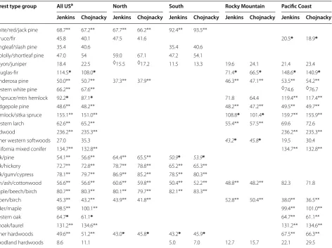
To examine the drivers of those differences, we car-ried out equivalence tests by forest type group at both the national and regional levels on the mean density of car-bon in aboveground live trees; a summary of the results

(3)

is given in Table 1. The quantity tested is mean differ-ence (Chojnacky − Jenkins) in plot level tonnes carbon per hectare; the test for equivalence was based on the percentage difference relative to the Jenkins based esti-mate (i.e. 100 × ((Chojnacky − Jenkins)/Jenkins)). The 5 (or 10) % of Jenkins, which was set as the equivalence interval, was put in units of tonnes per hectare for com-parison with the 95 % confidence interval for the α = 0.05 (or α = 0.1) two one-sided tests (TOST) of equivalence. Of the 26 forest type groups included in the analysis, 20 are equivalent (at 5 or 10 %) at the national level, with most equivalent at 5 %. The exceptions are: spruce/fir, longleaf/slash pine, loblolly/shortleaf pine, pinyon/juni-per, other western softwoods, and woodland hardwoods. At a regional level, differences emerge; in the North, only spruce/fir and loblolly/shortleaf pine are not equiva-lent (too few plots were available in pinyon/juniper for a reliable test statistic) while in the South, the pine types lacked equivalence, as did pinyon/juniper. This is very likely a reflection of the fact that the Chojnacky equations divide some taxa by specific gravity, while the Jenkins equations do not; softwoods generally display a larger range of specific gravity values within a species group than do hardwoods [14]. Researchers have noted con-siderable variability in the estimates produced by differ-ent southern pine biomass equations [15], even between different sets of local equations. Specific gravity, as men-tioned above, is a factor, (southern pines exhibit con-siderable variability in specific gravity), as well as stand origin, and the mathematical form of the equation itself. Melson et al. [16], in their investigation of the effects of model selection on carbon stock estimates in northwest

Oregon, noted that the national level Jenkins [1] equa-tions produced biomass estimates for Picea that were consistently lower than from approaches developed by the investigators, and hypothesized that differences in form between Picea species introduced bias into the gen-eralized equation.

Pinyon/juniper was not equivalent in any region in which it was tested. While fir/spruce/mountain hemlock was not equivalent in the Rocky Mountains, the stock estimates were equivalent to 5 % in the Pacific Coast region, likely a function of the species and size classes that dominate the groups in each of these regions. The elm/ash/cottonwood category is represented in each region, and was equivalent to 5 % in all areas except the Pacific Coast. The woodland class has been less well stud-ied than the others, and so less data and fewer equations are available to construct generalized equations like those in Jenkins et al. [1] and Chojnacky et al. [12]. Conse-quently, the woodland equations are not equivalent at the national level or in any region.

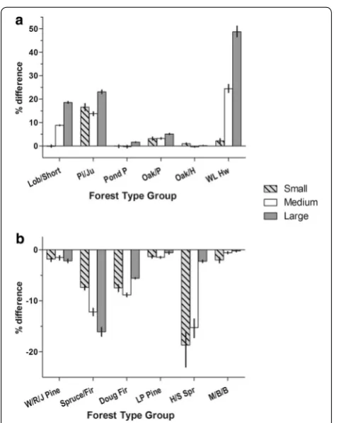
We also explored the effect of size class on equation performance, testing each combination of forest type group and stand size class and found notable differences among size classes, though no evidence of a systematic pattern. A summary of the results is given in Fig. 3a and

3b; the error bars represent the 95 % confidence inter-val transformed to percentage. Not every combination is shown; groups with results similar to another or com-prising a very small proportion of plots are not included. While some groups such as ponderosa pine, oak/hickory, lodgepole pine, and white/red/jack pine show small dif-ferences between size classes and are equivalent (or nearly so), others such as loblolly/shortleaf pine, longleaf/ slash pine (data not shown), woodland hardwoods, and spruce/fir show a strong pattern of increasing differences with increasing stand size, with a lack of equivalence between the small and large sawtimber classes. Note that both the direction and magnitude of the differences were variable across the forest type groups. Hemlock/Sitka spruce displayed a strong trend in the opposite direc-tion, with large differences between the two approaches for the small and medium size classes, and a very small difference in the large sawtimber class. The differ-ence between the two sets of estimates for the wood-land group that is shown in Table 1 is readily apparent in Fig. 3a, with a large increase in the percent difference as the stand size class increases. This may be due to the lack of woodland biomass equations based on diameter at root collar (drc) and the difficulty of obtaining accurate drc measurements. Bragg [17] and Bragg and McElligott [15] have discussed the importance of diameter at breast height (dbh) in some detail, comparing the performance of local, regional, and national equations for southern Fig. 2 Effect of the Chojnacky et al. [12] species groups and biomass

(4)

pines across a range of diameters. While most equations returned fairly similar estimates for trees up to 50 cm dbh, equation behavior diverged at larger diameters, in some cases returning estimates that were considerably different. In these examples, the national level Jenkins equations [1] did not produce extreme estimates, they were intermediate to those returned by local and regional equations. Melson et al. [16] also noted that consider-able error could be introduced when applying equations to trees with a dbh value outside the range on which the equations were developed.

Equivalence was not tested at the level of the individ-ual tree, though a random subset of individindivid-ual tree esti-mates were plotted for each species group to compare tree-level biomass estimates. These plots reflect the pat-terns demonstrated above, with one method producing

values consistently higher or lower than the other, the differences becoming more apparent at larger diam-eters. Tree data were also classified by east and west to further explore equation behavior within species groups where there are considerable differences in the range of tree diameters, east versus west. In many cases, no trends were revealed, but there are some key differences; a nota-ble example is shown in Fig. 4a, b, which show the results of tree-level carbon estimates by each set of equations, categorized as east and west. In Fig. 4a, the eastern US, the Jenkins estimates are larger than those produced from the Chojnacky equations, while in Fig. 4b, the west-ern US, the Jenkins estimates are generally somewhat lower, with the exception of the “Abies; LoSG” group. Figure 5 shows similar data for the woodland taxa; again, there is a considerable difference between the estimates

Table 1 Mean stock of carbon in aboveground live tree biomass as computed using the equations from Jenkins et al. [1] and Chojnacky et al. [12]

Values followed by a double asterisk (**) are equivalent at 5 %; values followed by a single asterisk (*) are equivalent at 10 %. Regions are as shown in Fig. 1. A diamond preceding a value indicates that the sample size was too small for a reliable test of equivalence. Data not shown for categories represented by fewer than 10 plots

a_{As shown in Fig.}₁

Forest type group All USa _North _South _{Rocky Mountain} _{Pacific Coast} Jenkins Chojnacky Jenkins Chojnacky Jenkins Chojnacky Jenkins Chojnacky Jenkins Chojnacky

White/red/jack pine 68.7** 67.2** 67.7** 66.2** 92.4** 93.5**

Spruce/fir 45.8 40.1 47.5 41.6 20.5* 18.9*

Longleaf/slash pine 35.4 40.6 35.4 40.6 Loblolly/shortleaf pine 47.0 54 59.0 67.1 47.2 54.1

Pinyon/juniper 18.4 22.5 ◊15.5 ◊17.2 11.5 13.3 19.6 24.1 21.4 23.4 Douglas-fir 114.5* 108.0* 71.4* 66.5* 148.6* 140.9*

Ponderosa pine 50.0** 50.7** 37.3** 37.9** 46.3** 47.1** 53.5** 54.2** Western white pine 66.2** 67.6** ◊74.6 ◊76.7 Fir/spruce/mtn hemlock 92.2* 87.1* 71.8 64.4 119.4** 117.4** Lodgepole pine 48.6** 48.2** 48.2** 47.2** 49.5** 49.7** Hemlock/sitka spruce 155.1** 151.0** 108.8* 101.4* 159.7** 155.9** Western larch 62.6** 65.2** 55.4** 57.5** 69.6 72.6 Redwood 236.2** 235.3** 236.2** 235.3** Other western softwoods 27.0 35.3 43.2* 45.8* 19.5 30.4 California mixed conifer 134.7** 132.8** 134.7** 132.8** Oak/pine 54.1** 56.6** 64.4** 65.5** 50.9* 53.9*

Oak/hickory 72.7** 72.8** 78.7** 78.8** 65.2** 65.3** Oak/gum/cypress 78.1** 79.7** 86.9** 85.2** 78.5** 80.3**

Elm/ash/cottonwood 56.6** 56.6** 60.6** 59.8** 50.4** 52.2** 48.8** 48.2** 82.3 71.8 Maple/beech/birch 80.7** 80.3** 80.1** 79.7** 82.1** 83.3**

(5)

computed with the two methods, with the Jenkins equa-tions producing consistently lower estimates than the Chojnacky equations. In this case, we see no obvious dif-ferences between the predictions in the East or West.

As mentioned above, the belowground component equations were also revised in the 2014 publication, and while not divided according to hardwood and softwood, the revised root component equations are subdivided by coarse and fine roots. There are important differences in the shape of the root component curve between the two approaches (Fig. 6), and the Jenkins hardwood equation yields a consistently lower proportion than the jnacky equation. This suggests that adopting the Cho-jnacky estimates for full above- and belowground tree would add up to an additional 2–3 % of biomass for hard-woods but would also affect some softwood estimates.

A preliminary analysis did show an effect on the test for the 5 % equivalence for some categories. However, our emphases here are the various species groups/equations and not the components.

Conclusions

The revised approach to developing these biomass equa-tions has the effect of providing better regional differen-tiation/representation at the plot/stand level summaries by allowing for separation within the taxonomic classes according to wood properties or growth habit. The emer-gence of Southern pines as distinctly different under the Chojnacky groups is one example. It is challeng-ing to provide specific criteria for chooschalleng-ing one set of equations over the other, since validating any biomass equation requires the destructive sampling of multi-ple stems across a range of diameters. The Chojnacky groups appear to provide greater resolution across for-est types and regions. From this, invfor-estigators working in southern pine, northern spruce-fir, pinyon-juniper, and woodland types may be advised to use the updated equa-tions [12], which provide more taxonomic resolution. It should also be noted that estimates of change over time Fig. 3 Effect of the two alternate biomass equations as relative

difference in stock (panel a, positive difference, panel b, negative). Estimates are classified by forest type group and stand size class. The

error bar represents the confidence interval used in the equivalence tests. In general, small stands have at least 50 % of stocking in small diameter trees, large stands have at least 50 % of stocking in large and medium diameter trees, with large tree stocking ≥ medium tree. The 12 forest type groups included here are: loblolly/shortleaf pine, pinyon/juniper, ponderosa pine, oak/pine, oak/hickory, and woodland hardwoods in panel a, and white/red/jack pine, spruce/fir, Douglas-fir, lodgepole pine, hemlock/Sitka spruce, and maple/beech/ birch in panel b

(6)

are somewhat less sensitive to equation choice than stock estimates, so if change is the primary variable of interest, the user can select either equation set, based on personal preference.

Individual large diameter trees can be very differ-ent—Chojnacky relative to Jenkins—given the general trends of the tree-level estimates (Figs. 4 and 5 in this manuscript as well as Figs. 2, 3, and 4 in Chojnacky et al. [12]). This effect of one or a very few larger trees can result in very different estimates even in an “equiva-lent” forest type group, and this potential for larger dif-ferences is reflected in plot-level data. For example, in some eastern hardwood type groups, which were consist-ently identified as equivalent, up to one-third of the plots were individually more than 5 % different. The oak/gum/ cypress type group in the South had 8 % of the plots with greater carbon density by over 5 % with the Jenkins esti-mates, while 27 % of plots had over 5 % greater carbon.

The remaining 65 % of the individual plots are within the 5 % bounds (data not shown here). This is consistent with our observation about similarities between the two sets and scale (Fig. 2)—the sometimes obvious and large dif-ferences for some forest type groups (all scales) become obscured when summed to total live tree carbon for the US. Singling out the correct or most accurate equations is beyond the scope here; however, caution is always war-ranted when applying equations to trees that are consid-erably outside the range of diameters used to construct the equations [16].

Our results point to a few forest type groups that are clearly not equivalent—southern pines, northern spruce-fir, and lower productivity arid western forests—while the majority of forest type groups are generally equiva-lent at the scales presented. Overall, the possibility of very different results between the Chojnacky and Jenkins sets decreases with aggregate summaries of those ‘equiv-alent’ type groups.

Methods Tree data source

In order to implement the revised biomass equations and identify applications where they are effectively inter-changeable, or equivalent, we used the Forest Inventory and Analysis Data Base (FIADB) compiled by the Forest Inventory and Analysis (FIA) Program of the US Forest Service [13]. The data are based on continuous system-atic annualized sampling of US forest lands, which are then compiled and made available by the FIA program of the US Forest Service [18]; the specific data in use here were downloaded from http://apps.fs.fed.us/fiadb-down-loads/datamart.html on 02 June 2015. Surveys are organ-ized and conducted on a large system of permanent plots over all land within individual states so that a portion of the survey data is collected each year on a continuous cycle, with remeasurement at 5 or 10 years depending on the state. The portion of the data used here include the conterminous United States (i.e., 48 states), and the por-tion of southern coastal Alaska that has the established permanent annual survey plots (the gray areas in Fig. 1).

Our focus here is on the tree data of the FIADB, and for this analysis we present the Chojnacky and Jenkins estimates in terms of carbon mass (i.e., kg carbon per tree or tonnes per hectare per plot). We use the entire tree data table to assure that all applicable species (the gray areas in Fig. 1) are represented. All other summa-ries are based on the most recent (most up-to-date) set of tree and plot data available per state, with the Cho-jnacky and Jenkins estimates expressed as tonnes of car-bon per hectare in live trees on forest inventory plots. These plot-level values are expanded to population totals, that is, total carbon stock per state, as provided Fig. 5 Examples of the Chojnacky-based and Jenkins-based

esti-mates for aboveground carbon mass (kg) of individual live trees by dbh. This example includes all trees within the woodland species group of Jenkins (black) and their mapping to Chojnacky species groups (not identified) in the East (red, North and South) and the West (blue, Pacific Coast and Rocky Mountain). Data points include all applicable live trees in the FIADB tree data table up to the 99th percentile of diameters in the East and West, respectively

(7)

within the FIADB as the basis for the result presented in Fig. 2. A subset of the current forest plot level sum-maries where the entire plot is identified as forested (i.e., single condition forest plots) is the basis for the results provided in Table 1 and Fig. 3.

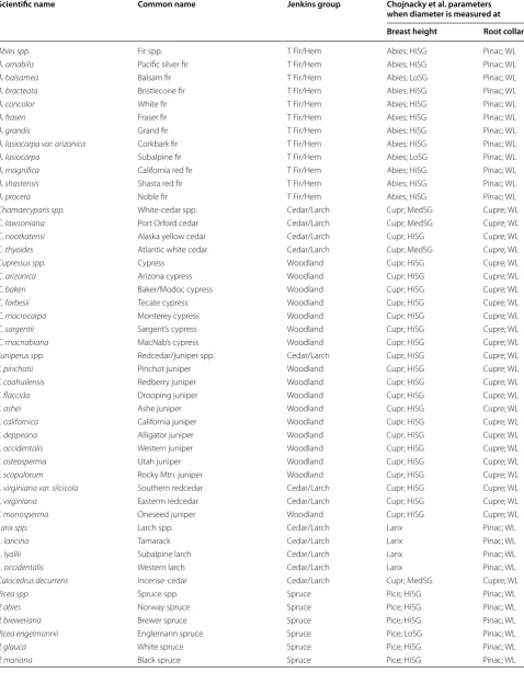
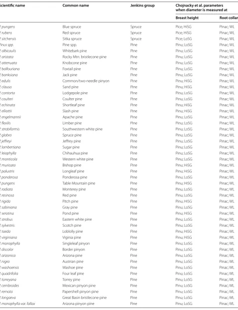
Application of Chojnacky et al. [12] to the FIADB

Chojnacky et al. [12] provided a revised and expanded set of biomass equations following the approach of Jenkins et al. [1]. The revised equations are based on an approach similar to that of Jenkins et al. [1] and with an expanded database of published biomass equations; see Chojnacky et al. [12] for details. The new set of 35 Chojnacky spe-cies groups are based on taxon (family or genera), growth habit, or average wood density. See Table 2 for the links between species in the FIADB and the Jenkins and Cho-jnacky classifications. This allocation to the newer cat-egories is not a simple mapping of the 10 Jenkins groups to Chojnacky groups. That is, while Jenkins groups are split among Chojnacky groups, so also the Chojnacky groups are in some cases composed of species from dif-ferent Jenkins groups. While Chojnacky et al. [12] devel-oped the set of new groups based on the FIADB, similar to Jenkins et al. [1], a very small percentage of hardwood species were not explicitly named (i.e., families were not listed [12]). We assigned these to the “Cor/Eri/Lau/Etc” group (Table 2).

In order to systematically assign all the biomass esti-mates presented in Chojnacky et al. [12] to trees in the FIADB (as in this analysis), we present a short set of steps to make this link. Note that these include our interpreta-tion of some of the assignments of species to groups that are not explicit such as some assignments to the wood-land groups or allocation to deciduous versus evergreen. These seven steps, which also include application of the revised root component, are the basis for the biomass equation group assignments in Table 2. Note that tables and figures referenced in this list refer to those in Cho-jnacky et al. [12]:

1. Overall, follow the placement of taxa as suggested within the manuscript (i.e., as in Tables 2, 3, 4, and Figs. 2, 3, and 4).

2. If a tree record is one of the five families (of Table 4) and the tree diameter is measured as diameter at root collar then one of the Table 4 woodland equations applies. Otherwise, if one of the five (Table 4) families and diameter is dbh then use the appropriate equa-tion from Tables 2 or 3. If not one of the five Table 4 families but tree diameter is provided as a root col-lar measurement, then convert drc to dbh follow-ing information provided in Fig. 1 before applying a Table 2 or 3 equation.

3. The calculations for the woodland (Table 4) Cupres-saceae (“Cupre; WL”) uses the “2nd juniper” equation from footnote #2 in Table 5.

4. The Fabaceae/Juglandaceae split into the two groups—“Fab/Jug/Carya” and “Fab/Jug”—is accord-ing to the genus Carya versus all others (i.e., not-Carya).

5. Fagaceae’s deciduous/evergreen split—“Faga; Decid” and “Faga; Evergrn”—sets deciduous as the default. The Fagaceae allocated to evergreen are those five species explicitly listed as evergreen in Table 3 and those identified as evergreen from the USDA PLANTS database [19], which currently includes the addition of three live oak species.

6. The 6-family general equation at the middle of page 136 (in Table 3 of Chojnacky et al. [12])—“Cor/Eri/ Lau/Etc”—is assigned trees by family from 3 sources: (a) the six families listed in Table 3; (b) the five addi-tional families noted in the Fig. 3 caption, and (c) any additional formerly unassigned hardwood species. 7. Roots—the Chojnacky estimates use both of the

belowground root equations of Table 6 (the sum of the two is generally equivalent to the original Jen-kins root component). Note these are dbh-based, so a drc tree should first convert drc-to-dbh according to Fig. 1. Also note, all other (other than root) com-ponents of the original Jenkins et al. [1] are applicable here.

Identifying equivalence between the alternate biomass estimates

(8)

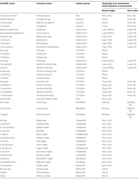
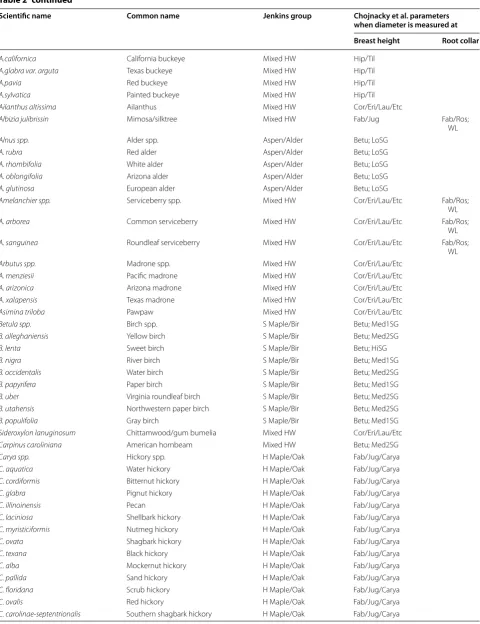
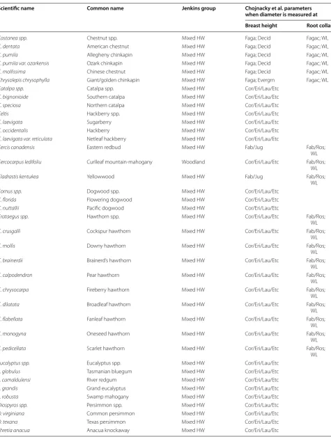
Table 2 Guide to applying Chojnacky species groups (as shown in Table 5, Chojnacky et al. [12]) to US species

Scientific name Common name Jenkins group Chojnacky et al. parameters when diameter is measured at Breast height Root collar

Abies spp. Fir spp. T Fir/Hem Abies; HiSG Pinac; WL

A. amabilis Pacific silver fir T Fir/Hem Abies; HiSG Pinac; WL

A. balsamea Balsam fir T Fir/Hem Abies; LoSG Pinac; WL

A. bracteata Bristlecone fir T Fir/Hem Abies; HiSG Pinac; WL

A. concolor White fir T Fir/Hem Abies; HiSG Pinac; WL

A. fraseri Fraser fir T Fir/Hem Abies; HiSG Pinac; WL

A. grandis Grand fir T Fir/Hem Abies; HiSG Pinac; WL

A. lasiocarpa var. arizonica Corkbark fir T Fir/Hem Abies; HiSG Pinac; WL

A. lasiocarpa Subalpine fir T Fir/Hem Abies; LoSG Pinac; WL

A. magnifica California red fir T Fir/Hem Abies; HiSG Pinac; WL

A. shastensis Shasta red fir T Fir/Hem Abies; HiSG Pinac; WL

A. procera Noble fir T Fir/Hem Abies; HiSG Pinac; WL

Chamaecyparis spp. White-cedar spp. Cedar/Larch Cupr; MedSG Cupre; WL

C. lawsoniana Port Orford cedar Cedar/Larch Cupr; MedSG Cupre; WL

C. nootkatensi Alaska yellow cedar Cedar/Larch Cupr; HiSG Cupre; WL

C. thyoides Atlantic white cedar Cedar/Larch Cupr; MedSG Cupre; WL

Cupressus spp. Cypress Woodland Cupr; HiSG Cupre; WL

C. arizonica Arizona cypress Woodland Cupr; HiSG Cupre; WL

C. bakeri Baker/Modoc cypress Woodland Cupr; HiSG Cupre; WL

C. forbesii Tecate cypress Woodland Cupr; HiSG Cupre; WL

C. macrocarpa Monterey cypress Woodland Cupr; HiSG Cupre; WL

C. sargentii Sargent’s cypress Woodland Cupr; HiSG Cupre; WL

C. macnabiana MacNab’s cypress Woodland Cupr; HiSG Cupre; WL

Juniperus spp. Redcedar/juniper spp. Cedar/Larch Cupr; HiSG Cupre; WL

J. pinchotii Pinchot juniper Woodland Cupr; HiSG Cupre; WL

J. coahuilensis Redberry juniper Woodland Cupr; HiSG Cupre; WL

J. flaccida Drooping juniper Woodland Cupr; HiSG Cupre; WL

J. ashei Ashe juniper Woodland Cupr; HiSG Cupre; WL

J. californica California juniper Woodland Cupr; HiSG Cupre; WL

J. deppeana Alligator juniper Woodland Cupr; HiSG Cupre; WL

J. occidentalis Western juniper Woodland Cupr; HiSG Cupre; WL

J. osteosperma Utah juniper Woodland Cupr; HiSG Cupre; WL

J. scopulorum Rocky Mtn. juniper Woodland Cupr; HiSG Cupre; WL

J. virginiana var. silcicola Southern redcedar Cedar/Larch Cupr; HiSG Cupre; WL

J. virginiana Easterm redcedar Cedar/Larch Cupr; HiSG Cupre; WL

J. monosperma Oneseed juniper Woodland Cupr; HiSG Cupre; WL

Larix spp. Larch spp. Cedar/Larch Larix Pinac; WL

L. laricina Tamarack Cedar/Larch Larix Pinac; WL

L. lyallii Subalpine larch Cedar/Larch Larix Pinac; WL

L. occidentalis Western larch Cedar/Larch Larix Pinac; WL

Calocedrus decurrens Incense-cedar Cedar/Larch Cupr; MedSG Cupre; WL

Picea spp. Spruce spp. Spruce Pice; HiSG Pinac; WL

P. abies Norway spruce Spruce Pice; HiSG Pinac; WL

P. breweriana Brewer spruce Spruce Pice; HiSG Pinac; WL

Picea engelmannii Englemann spruce Spruce Pice; LoSG Pinac; WL

P. glauca White spruce Spruce Pice; HiSG Pinac; WL

(9)

Table 2 continued

P. pungens Blue spruce Spruce Pice; HiSG Pinac; WL

P. rubens Red spruce Spruce Pice; HiSG Pinac; WL

P. sitchensis Sitka spruce Spruce Pice; LoSG Pinac; WL

Pinus spp. Pine spp. Pine Pinu; LoSG Pinac; WL

P. albicaulis Whitebark pine Pine Pinu; LoSG Pinac; WL

P. aristata Rocky Mtn. bristlecone pine Pine Pinu; LoSG Pinac; WL

P. attenuata Knobcone pine Pine Pinu; LoSG Pinac; WL

P. balfouriana Foxtail pine Pine Pinu; LoSG Pinac; WL

P. banksiana Jack pine Pine Pinu; LoSG Pinac; WL

P. edulis Common/two-needle pinyon Pine Pinu; HiSG Pinac; WL

P. clausa Sand pine Pine Pinu; HiSG Pinac; WL

P. contorta Lodgepole pine Pine Pinu; LoSG Pinac; WL

P. coulteri Coulter pine Pine Pinu; LoSG Pinac; WL

P. echinata Shortleaf pine Pine Pinu; HiSG Pinac; WL

P. elliottii Slash pine Pine Pinu; HiSG Pinac; WL

P. engelmannii Apache pine Pine Pinu; LoSG Pinac; WL

P. flexilis Limber pine Pine Pinu; LoSG Pinac; WL

P. strobiformis Southwestern white pine Pine Pinu; LoSG Pinac; WL

P. glabra Spruce pine Pine Pinu; LoSG Pinac; WL

P. jeffreyi Jeffrey pine Pine Pinu; LoSG Pinac; WL

P. lambertiana Sugar pine Pine Pinu; LoSG Pinac; WL

P. leiophylla Chihauhua pine Pine Pinu; LoSG Pinac; WL

P. monticola Western white pine Pine Pinu; LoSG Pinac; WL

P. muricata Bishop pine Pine Pinu; HiSG Pinac; WL

P. palustris Longleaf pine Pine Pinu; HiSG Pinac; WL

P. ponderosa Ponderosa pine Pine Pinu; LoSG Pinac; WL

P. pungens Table Mountain pine Pine Pinu; HiSG Pinac; WL

P. radiata Monterey pine Pine Pinu; LoSG Pinac; WL

P. resinosa Red pine Pine Pinu; LoSG Pinac; WL

P. rigida Pitch pine Pine Pinu; HiSG Pinac; WL

P. sabiniana Gray pine Pine Pinu; LoSG Pinac; WL

P. serotina Pond pine Pine Pinu; HiSG Pinac; WL

P. strobus Eastern white pine Pine Pinu; LoSG Pinac; WL

P. sylvestris Scotch pine Pine Pinu; LoSG Pinac; WL

P. taeda Loblolly pine Pine Pinu; HiSG Pinac; WL

P. virginiana Viginia pine Pine Pinu; HiSG Pinac; WL

P. monophylla Singleleaf pinyon Pine Pinu; LoSG Pinac; WL

P. discolor Border pinyon Pine Pinu; LoSG Pinac; WL

P. arizonica Arizona pine Pine Pinu; LoSG Pinac; WL

P. nigra Austrian pine Pine Pinu; LoSG Pinac; WL

P. washoensis Washoe pine Pine Pinu; LoSG Pinac; WL

P. quadrifolia Four leaf pine Pine Pinu; LoSG Pinac; WL

P. torreyana Torrey pine Pine Pinu; LoSG Pinac; WL

P. cembroides Mexican pinyon pine Pine Pinu; LoSG Pinac; WL

P. remota Papershell pinyon pine Pine Pinu; LoSG Pinac; WL

P. longaeva Great Basin bristlecone pine Pine Pinu; LoSG Pinac; WL

(10)

P. elliottii var. elliottii Honduras pine Pine Pinu; LoSG Pinac; WL

Pseudotsuga spp. Douglas-fir spp. Doug Fir Pseud Pinac; WL

P. macrocarpa Bigcone Douglas-fir Doug Fir Pseud Pinac; WL

P. menziesii Douglas-fir Doug Fir Pseud Pinac; WL

Sequoia sempervirens Redwood Cedar/Larch Cupr; MedSG Cupre; WL

Sequoiadendron giganteum Giant sequoia Cedar/Larch Cupr; MedSG Cupre; WL

Taxodium spp. Baldcypress spp. Cedar/Larch Cupr; HiSG Cupre; WL

T. distichum Baldcypress Cedar/Larch Cupr; HiSG Cupre; WL

T. ascendens Pondcypress Cedar/Larch Cupr; HiSG Cupre; WL

T. mucronatum Montezuma baldcypress Cedar/Larch Cupr; HiSG Cupre; WL

Taxus spp. Yew spp. T Fir/Hem Pseud

T. brevifolia Pacific yew T Fir/Hem Pseud

T. floridana Florida yew T Fir/Hem Pseud

Thuja spp. Thuja spp. Cedar/Larch Cupr; MedSG Cupre; WL

T. occidentalis Northern white-cedar Cedar/Larch Cupr; LoSG Cupre; WL

T. plicata Western redcedar Cedar/Larch Cupr; MedSG Cupre; WL

Torreya spp. Torreya (nutmeg) spp. T Fir/Hem Pseud

T. californica California torreya T Fir/Hem Pseud

T. taxifolia Florida torreya T Fir/Hem Pseud

Tsuga spp. Hemlock spp. T Fir/Hem Tsug; HiSG Pinac; WL

T. canadensis Eastern hemlock T Fir/Hem Tsug; LoSG Pinac; WL

T. caroliniana Carolina hemlock T Fir/Hem Tsug; HiSG Pinac; WL

T. heterophylla Western hemlock T Fir/Hem Tsug; HiSG Pinac; WL

T. mertensiana Mountain hemlock T Fir/Hem Tsug; HiSG Pinac; WL

Dead conifer Unknown dead conifer Pine Pinu; LoSG

Acacia spp. Acacia spp. Woodland Fab/Jug Fab/Ros;

WL

A. farnesiana Sweet acacia Woodland Fab/Jug Fab/Ros;

WL

A. greggii Catclaw acacia Woodland Fab/Jug Fab/Ros;

WL

Acer spp. Maple spp. S Maple/Bir Acer; LoSG

A. barbatum Florida maple S Maple/Bir Acer; HiSG

A. macrophyllum Bigleaf maple S Maple/Bir Acer; LoSG

A. negundo Boxelder S Maple/Bir Acer; LoSG

A. nigrum Black maple H Maple/Oak Acer; HiSG

A. pensylvanicum Striped maple S Maple/Bir Acer; LoSG

A. rubrum Red maple S Maple/Bir Acer; LoSG

A. saccharinum Silver maple S Maple/Bir Acer; LoSG

A. saccharum Sugar maple H Maple/Oak Acer; HiSG

A. spicatum Mountain maple S Maple/Bir Acer; LoSG

A. platanoides Norway maple S Maple/Bir Acer; LoSG

A. glabrum Rocky Mtn. maple Woodland Acer; LoSG

A. grandidentatum Bigtooth maple Woodland Acer; LoSG

A. leucoderme Chalk maple Mixed HW Acer; LoSG

Aesculus spp. Buckeye spp. Mixed HW Hip/Til

A.glabra Ohio buckeye Mixed HW Hip/Til

(11)

A.californica California buckeye Mixed HW Hip/Til

A.glabra var. arguta Texas buckeye Mixed HW Hip/Til

A.pavia Red buckeye Mixed HW Hip/Til

A.sylvatica Painted buckeye Mixed HW Hip/Til

Ailanthus altissima Ailanthus Mixed HW Cor/Eri/Lau/Etc

Albizia julibrissin Mimosa/silktree Mixed HW Fab/Jug Fab/Ros;

WL

Alnus spp. Alder spp. Aspen/Alder Betu; LoSG

A. rubra Red alder Aspen/Alder Betu; LoSG

A. rhombifolia White alder Aspen/Alder Betu; LoSG

A. oblongifolia Arizona alder Aspen/Alder Betu; LoSG

A. glutinosa European alder Aspen/Alder Betu; LoSG

Amelanchier spp. Serviceberry spp. Mixed HW Cor/Eri/Lau/Etc Fab/Ros;

WL

A. arborea Common serviceberry Mixed HW Cor/Eri/Lau/Etc Fab/Ros;

WL

A. sanguinea Roundleaf serviceberry Mixed HW Cor/Eri/Lau/Etc Fab/Ros;

WL

Arbutus spp. Madrone spp. Mixed HW Cor/Eri/Lau/Etc

A. menziesii Pacific madrone Mixed HW Cor/Eri/Lau/Etc

A. arizonica Arizona madrone Mixed HW Cor/Eri/Lau/Etc

A. xalapensis Texas madrone Mixed HW Cor/Eri/Lau/Etc

Asimina triloba Pawpaw Mixed HW Cor/Eri/Lau/Etc

Betula spp. Birch spp. S Maple/Bir Betu; Med1SG

B. alleghaniensis Yellow birch S Maple/Bir Betu; Med2SG

B. lenta Sweet birch S Maple/Bir Betu; HiSG

B. nigra River birch S Maple/Bir Betu; Med1SG

B. occidentalis Water birch S Maple/Bir Betu; Med2SG

B. papyrifera Paper birch S Maple/Bir Betu; Med1SG

B. uber Virginia roundleaf birch S Maple/Bir Betu; Med2SG

B. utahensis Northwestern paper birch S Maple/Bir Betu; Med2SG

B. populifolia Gray birch S Maple/Bir Betu; Med1SG

Sideroxylon lanuginosum Chittamwood/gum bumelia Mixed HW Cor/Eri/Lau/Etc

Carpinus caroliniana American hornbeam Mixed HW Betu; Med2SG

Carya spp. Hickory spp. H Maple/Oak Fab/Jug/Carya

C. aquatica Water hickory H Maple/Oak Fab/Jug/Carya

C. cordiformis Bitternut hickory H Maple/Oak Fab/Jug/Carya

C. glabra Pignut hickory H Maple/Oak Fab/Jug/Carya

C. illinoinensis Pecan H Maple/Oak Fab/Jug/Carya

C. laciniosa Shellbark hickory H Maple/Oak Fab/Jug/Carya

C. myristiciformis Nutmeg hickory H Maple/Oak Fab/Jug/Carya

C. ovata Shagbark hickory H Maple/Oak Fab/Jug/Carya

C. texana Black hickory H Maple/Oak Fab/Jug/Carya

C. alba Mockernut hickory H Maple/Oak Fab/Jug/Carya

C. pallida Sand hickory H Maple/Oak Fab/Jug/Carya

C. floridana Scrub hickory H Maple/Oak Fab/Jug/Carya

C. ovalis Red hickory H Maple/Oak Fab/Jug/Carya

(12)

Castanea spp. Chestnut spp. Mixed HW Faga; Decid Fagac; WL

C. dentata American chestnut Mixed HW Faga; Decid Fagac; WL

C. pumila Allegheny chinkapin Mixed HW Faga; Decid Fagac; WL

C. pumila var. ozarkensis Ozark chinkapin Mixed HW Faga; Decid Fagac; WL

C. mollissima Chinese chestnut Mixed HW Faga; Decid Fagac; WL

Chrysolepis chrysophylla Giant/golden chinkapin Mixed HW Faga; Evergrn Fagac; WL

Catalpa spp. Catalpa spp. Mixed HW Cor/Eri/Lau/Etc

C. bignonioide Southern catalpa Mixed HW Cor/Eri/Lau/Etc

C. speciosa Northern catalpa Mixed HW Cor/Eri/Lau/Etc

Celtis Hackberry spp. Mixed HW Cor/Eri/Lau/Etc

C. laevigata Sugarberry Mixed HW Cor/Eri/Lau/Etc

C. occidentalis Hackberry Mixed HW Cor/Eri/Lau/Etc

C. laevigata var. reticulata Netleaf hackberry Mixed HW Cor/Eri/Lau/Etc

Cercis canadensis Eastern redbud Mixed HW Fab/Jug Fab/Ros;

WL

Cercocarpus ledifoliu Curlleaf mountain-mahogany Woodland Cor/Eri/Lau/Etc Fab/Ros;

WL

Cladrastis kentukea Yellowwood Mixed HW Fab/Jug Fab/Ros;

WL

Cornus spp. Dogwood spp. Mixed HW Cor/Eri/Lau/Etc

C. florida Flowering dogwood Mixed HW Cor/Eri/Lau/Etc

C. nuttallii Pacific dogwood Mixed HW Cor/Eri/Lau/Etc

Crataegus spp. Hawthorn spp. Mixed HW Cor/Eri/Lau/Etc Fab/Ros;

WL

C. crusgalli Cockspur hawthorn Mixed HW Cor/Eri/Lau/Etc Fab/Ros;

WL

C. mollis Downy hawthorn Mixed HW Cor/Eri/Lau/Etc Fab/Ros;

WL

C. brainerdii Brainerd’s hawthorn Mixed HW Cor/Eri/Lau/Etc Fab/Ros;

WL

C. calpodendron Pear hawthorn Mixed HW Cor/Eri/Lau/Etc Fab/Ros;

WL

C. chrysocarpa Fireberry hawthorn Mixed HW Cor/Eri/Lau/Etc Fab/Ros;

WL

C. dilatata Broadleaf hawthorn Mixed HW Cor/Eri/Lau/Etc Fab/Ros;

WL

C. flabellata Fanleaf hawthorn Mixed HW Cor/Eri/Lau/Etc Fab/Ros;

WL

C. monogyna Oneseed hawthorn Mixed HW Cor/Eri/Lau/Etc Fab/Ros;

WL

C. pedicellata Scarlet hawthorn Mixed HW Cor/Eri/Lau/Etc Fab/Ros;

WL

Eucalyptus spp. Eucalyptus spp. Mixed HW Cor/Eri/Lau/Etc

E. globulus Tasmanian bluegum Mixed HW Cor/Eri/Lau/Etc

E. camaldulensi River redgum Mixed HW Cor/Eri/Lau/Etc

E. grandis Grand eucalyptus Mixed HW Cor/Eri/Lau/Etc

E. robusta Swamp mahogany Mixed HW Cor/Eri/Lau/Etc

Diospyros spp. Persimmon spp. Mixed HW Cor/Eri/Lau/Etc

D. virginiana Common persimmon Mixed HW Cor/Eri/Lau/Etc

D. texana Texas persimmon Mixed HW Cor/Eri/Lau/Etc

(13)

Fagus grandifolia American beech H Maple/Oak Faga; Decid Fagac; WL

Fraxinus spp. Ash spp. Mixed HW Olea; LoSG

F. americana White ash Mixed HW Olea; HiSG

F. latifolia Oregon ash Mixed HW Olea; LoSG

F. nigra Black ash Mixed HW Olea; LoSG

F. pennsylvanica Green ash Mixed HW Olea; LoSG

F. profunda Pumpkin ash Mixed HW Olea; LoSG

F. quadrangulata Blue ash Mixed HW Olea; LoSG

F. velutina Velvet ash Mixed HW Olea; LoSG

F. caroliniana Carolina ash Mixed HW Olea; LoSG

F. texensis Texas ash Mixed HW Olea; LoSG

Gleditsia spp. Honeylocust spp. Mixed HW Fab/Jug Fab/Ros;

WL

G. aquatica Waterlocust Mixed HW Fab/Jug Fab/Ros;

WL

G. triacanthos Honeylocust Mixed HW Fab/Jug Fab/Ros;

WL

Gordonia lasianthus Loblolly-bay Mixed HW Cor/Eri/Lau/Etc

Ginkgo biloba Ginkgo Mixed HW Cor/Eri/Lau/Etc

Gymnocluadus diocicus Kentucky coffeetree Mixed HW Fab/Jug Fab/Ros;

WL

Halesia spp. Silverbell spp. Mixed HW Cor/Eri/Lau/Etc

H. carolina Carolina silverbell Mixed HW Cor/Eri/Lau/Etc

H. diptera Two-wing silverbell Mixed HW Cor/Eri/Lau/Etc

H. parviflora Little silverbell Mixed HW Cor/Eri/Lau/Etc

Ilex opaca American holly Mixed HW Cor/Eri/Lau/Etc

Juglans spp. Walnut spp. Mixed HW Fab/Jug

J. cinerea Butternut Mixed HW Fab/Jug

J. nigra Black walnut Mixed HW Fab/Jug

J. hindsii No. California black walnut Mixed HW Fab/Jug

J. californica So. California black walnut Mixed HW Fab/Jug

J. microcarpa Texas walnut Mixed HW Fab/Jug

J. major Arizona walnut Mixed HW Fab/Jug

Liquidambar styraciflua Sweetgum Mixed HW Hama

Liriodendron tulipifera Yellow poplar Mixed HW Magno

Lithocarpus densiflorus Tanoak Mixed HW Faga; Evergrn Fagac; WL

Maclura pomifera Osage orange Mixed HW Cor/Eri/Lau/Etc

Magnolia spp. Magnolia spp. Mixed HW Magno

M. acuminata Cucumbertree Mixed HW Magno

M. grandiflora Southern magnolia Mixed HW Magno

M. virginiana Sweeetbay Mixed HW Magno

M. macrophylla Bigleaf magnolia Mixed HW Magno

M. fraseri Mountain/Frasier magnolia Mixed HW Magno

M. pyramidata Pyramid magnolia Mixed HW Magno

M. tripetala Umbrella magnolia Mixed HW Magno

Malus spp. Apple spp. Mixed HW Cor/Eri/Lau/Etc Fab/Ros;

WL

M. fusca Oregon crab apple Mixed HW Cor/Eri/Lau/Etc Fab/Ros;

(14)

M. angustifolia Southern crabapple Mixed HW Cor/Eri/Lau/Etc Fab/Ros;

WL

M. coronaria Sweet crabapple Mixed HW Cor/Eri/Lau/Etc Fab/Ros;

WL

M. ioensi Prairie crabapple Mixed HW Cor/Eri/Lau/Etc Fab/Ros;

WL

Morus spp. Mulberry spp. Mixed HW Cor/Eri/Lau/Etc

M. alba White mulberry Mixed HW Cor/Eri/Lau/Etc

M. rubra Red mulberry Mixed HW Cor/Eri/Lau/Etc

M. microphyll Texas mulberry Mixed HW Cor/Eri/Lau/Etc

M. nigra Black mulberry Mixed HW Cor/Eri/Lau/Etc

Nyssa spp. Tupelo spp. Mixed HW Cor/Eri/Lau/Etc

N. aquatica Water tupelo Mixed HW Cor/Eri/Lau/Etc

N. ogeche Ogeechee tupelo Mixed HW Cor/Eri/Lau/Etc

N. sylvatica Blackgum Mixed HW Cor/Eri/Lau/Etc

N. biflora Swamp tupelo Mixed HW Cor/Eri/Lau/Etc

Ostrya virginiana Eastern hophornbeam Mixed HW Betu; HiSG

Oxydendrum arboreum Sourwood Mixed HW Cor/Eri/Lau/Etc

Paulownia tomentosa Paulownia/empress tree Mixed HW Cor/Eri/Lau/Etc

Persea spp. Bay spp. Mixed HW Cor/Eri/Lau/Etc

Persea borbonia Redbay Mixed HW Cor/Eri/Lau/Etc

Planera aquatica Water elm/planetree Mixed HW Cor/Eri/Lau/Etc

Platanus spp. Sycamore spp. Mixed HW Cor/Eri/Lau/Etc

P. racemosa California sycamore Mixed HW Cor/Eri/Lau/Etc

P. occidentalis American sycamore Mixed HW Cor/Eri/Lau/Etc

P. wrightii Arizona sycamore Mixed HW Cor/Eri/Lau/Etc

Populus spp. Cottonwood/poplar spp. Aspen/Alder Sali; HiSG

P. balsamifera Balsam poplar Aspen/Alder Sali; LoSG

P. deltoides Eastern cottonwood Aspen/Alder Sali; HiSG

P. grandidentata Bigtooth aspen Aspen/Alder Sali; HiSG

P. heterophylla Swamp cottonwood Aspen/Alder Sali; HiSG

P. deltoides Plains cottonwood Aspen/Alder Sali; HiSG

P. tremuloides Quaking aspen Aspen/Alder Sali; HiSG

P. balsamifera Black cottonwood Aspen/Alder Sali; LoSG

P. fremontii Fremont cottonwood Aspen/Alder Sali; HiSG

P. angustifolia Narrlowleaf cottonwood Aspen/Alder Sali; HiSG

P. alba Silver poplar Aspen/Alder Sali; HiSG

P. nigra Lombardy poplar Aspen/Alder Sali; HiSG

Prosopis spp. Mesquite spp. Woodland Fab/Jug Fab/Ros;

WL

P. glandulosa Honey mesquite Woodland Fab/Jug Fab/Ros;

WL

P. velutina Velvet mesquite Woodland Fab/Jug Fab/Ros;

WL

P. pubescens Screwbean mesquite Woodland Fab/Jug Fab/Ros;

WL

Prunus spp. Cherry/plum spp. Mixed HW Cor/Eri/Lau/Etc Fab/Ros;

WL

P. pensylvanica Pin cherry Mixed HW Cor/Eri/Lau/Etc Fab/Ros;

(15)

P. serotina Black cherry Mixed HW Cor/Eri/Lau/Etc Fab/Ros;

WL

P. virginiana Chokecherry Mixed HW Cor/Eri/Lau/Etc Fab/Ros;

WL

P. persica Peach Mixed HW Cor/Eri/Lau/Etc Fab/Ros;

WL

P. nigra Canada plum Mixed HW Cor/Eri/Lau/Etc Fab/Ros;

WL

P. americana American plum Mixed HW Cor/Eri/Lau/Etc Fab/Ros;

WL

P. emarginata Bitter cherry Woodland Cor/Eri/Lau/Etc Fab/Ros;

WL

P. alleghaniensis Allegheny plum Mixed HW Cor/Eri/Lau/Etc Fab/Ros;

WL

P. angustifolia Chickasaw plum Mixed HW Cor/Eri/Lau/Etc Fab/Ros;

WL

P. avium Sweet cherry (domestic) Mixed HW Cor/Eri/Lau/Etc Fab/Ros;

WL

P. cerasus Sour cherry (domestic) Mixed HW Cor/Eri/Lau/Etc Fab/Ros;

WL

P. domestica European plum (domestic) Mixed HW Cor/Eri/Lau/Etc Fab/Ros;

WL

P. mahaleb Mahaleb cherry (domestic) Mixed HW Cor/Eri/Lau/Etc Fab/Ros;

WL

Quercus spp. Oak spp. H Maple/Oak Faga; Decid Fagac; WL

Q. agrifolia California live oak H Maple/Oak Faga; Evergrn Fagac; WL

Q. alba White oak H Maple/Oak Faga; Decid Fagac; WL

Q. arizonica Arizona white oak Woodland Faga; Decid Fagac; WL

Q. bicolor Swamp white oak H Maple/Oak Faga; Decid Fagac; WL

Q. chrysolepis Canyon live oak H Maple/Oak Faga; Decid Fagac; WL

Q. coccinea Scarlet oak H Maple/Oak Faga; Decid Fagac; WL

Q. douglasii Blue oak H Maple/Oak Faga; Evergrn Fagac; WL

Q. sinuata var. sinuata Durand oak H Maple/Oak Faga; Decid Fagac; WL

Q. ellipsoidalis Northern pin oak H Maple/Oak Faga; Decid Fagac; WL

Q. emoryi Emory oak Woodland Faga; Decid Fagac; WL

Q. engelmannii Englemann oak H Maple/Oak Faga; Decid Fagac; WL

Q. falcata Southern red oak H Maple/Oak Faga; Decid Fagac; WL

Q. pagoda Cherrybark oak H Maple/Oak Faga; Decid Fagac; WL

Q. gambelii Gambel oak Woodland Faga; Decid Fagac; WL

Q. garryana Oregon white oak H Maple/Oak Faga; Decid Fagac; WL

Q. ilicifolia Scrub oak H Maple/Oak Faga; Decid Fagac; WL

Q. imbricaria Shingle oak H Maple/Oak Faga; Decid Fagac; WL

Q. kelloggii California black oak H Maple/Oak Faga; Decid Fagac; WL

Q. laevis Turkey oak H Maple/Oak Faga; Decid Fagac; WL

Q. laurifolia Laurel oak H Maple/Oak Faga; Evergrn Fagac; WL

Q. lobata California white oak H Maple/Oak Faga; Decid Fagac; WL

Q. lyrata Overcup oak H Maple/Oak Faga; Decid Fagac; WL

Q. macrocarpa Bur oak H Maple/Oak Faga; Decid Fagac; WL

Q. marilandica Blackjack oak H Maple/Oak Faga; Decid Fagac; WL

(16)

Q. muehlenbergii Chinkapin oak H Maple/Oak Faga; Decid Fagac; WL

Q. nigra Water oak H Maple/Oak Faga; Decid Fagac; WL

Q. texana Texas red oak H Maple/Oak Faga; Decid Fagac; WL

Q. oblongifolia Mexican blue oak Woodland Faga; Decid Fagac; WL

Q. palustris Pin oak H Maple/Oak Faga; Decid Fagac; WL

Q. phellos Willow oak H Maple/Oak Faga; Decid Fagac; WL

Q. prinus Chestnut oak H Maple/Oak Faga; Decid Fagac; WL

Q. rubra Northern red oak H Maple/Oak Faga; Decid Fagac; WL

Q. shumardii Shumard oak H Maple/Oak Faga; Decid Fagac; WL

Q. stellata Post oak H Maple/Oak Faga; Decid Fagac; WL

Q. simili Delta post oak H Maple/Oak Faga; Decid Fagac; WL

Q. velutina Black oak H Maple/Oak Faga; Decid Fagac; WL

Q. virginiana Live oak H Maple/Oak Faga; Evergrn Fagac; WL

Q. wislizeni Interier live oak H Maple/Oak Faga; Evergrn Fagac; WL

Q. margarettiae Dwarf post oak H Maple/Oak Faga; Evergrn Fagac; WL

Q. minima Dwarf live oak H Maple/Oak Faga; Evergrn Fagac; WL

Q. incana Bluejack oak H Maple/Oak Faga; Decid Fagac; WL

Q. hypoleucoides Silverleaf oak Woodland Faga; Decid Fagac; WL

Q. oglethorpensis Oglethorpe oak H Maple/Oak Faga; Decid Fagac; WL

Q. prinoides Dwarf chinkapin oak H Maple/Oak Faga; Decid Fagac; WL

Q. grisea Gray oak Woodland Faga; Decid Fagac; WL

Q. rugosa Netleaf oak H Maple/Oak Faga; Decid Fagac; WL

Q. gracilliformis Chisos oak Woodland Faga; Decid Fagac; WL

Amyris elemifera Sea torchwood Mixed HW Cor/Eri/Lau/Etc

Annona glabra Pond apple Mixed HW Cor/Eri/Lau/Etc

Bursera simaruba Gumbo limbo Mixed HW Cor/Eri/Lau/Etc

Casuarina spp. Sheoak spp. Mixed HW Cor/Eri/Lau/Etc

C. glauca Gray sheoak Mixed HW Cor/Eri/Lau/Etc

C. lepidophloia Belah Mixed HW Cor/Eri/Lau/Etc

Cinnamomum camphora Camphortree Mixed HW Cor/Eri/Lau/Etc

Citharexylum fruticosum Florida fiddlewood Mixed HW Cor/Eri/Lau/Etc

Citrus spp. Citrus spp. Mixed HW Cor/Eri/Lau/Etc

Coccoloba diversifolia Tietongue/pigeon plum Mixed HW Cor/Eri/Lau/Etc

Colubrina elliptica Soldierwood Mixed HW Cor/Eri/Lau/Etc

Cordia sebestena Longleaf geigertree Mixed HW Cor/Eri/Lau/Etc

Cupaniopsis anacardioides Carrotwood Mixed HW Cor/Eri/Lau/Etc

Condalia hookeri Bluewood Woodland Cor/Eri/Lau/Etc

Ebenopsis ebano Blackbead ebony Woodland Fab/Jug Fab/Ros;

WL

Leucaena pulverulenta Great leadtree Woodland Fab/Jug Fab/Ros;

WL

Sophora affinis Texas sophora Woodland Fab/Jug Fab/Ros;

WL

Eugenia rhombea Red stopper Mixed HW Cor/Eri/Lau/Etc

Exothea paniculata Butterbough/inkwood Mixed HW Cor/Eri/Lau/Etc

Ficus aurea Florida strangler fig Mixed HW Cor/Eri/Lau/Etc

Ficus citrifolia Banyantree/shortleaf fig Mixed HW Cor/Eri/Lau/Etc

(17)

Hippomane mancinella Manchineel Mixed HW Cor/Eri/Lau/Etc

Lysiloma latisiliquum False tamarind Mixed HW Fab/Jug Fab/Ros;

WL

Mangifera indica Mango Mixed HW Cor/Eri/Lau/Etc

Metopium toxiferum Florida poisontree Mixed HW Cor/Eri/Lau/Etc

Piscidia piscipula Fishpoison tree Mixed HW Fab/Jug Fab/Ros;

WL

Schefflera actinophylla Octopus tree/schefflera Mixed HW Cor/Eri/Lau/Etc

Sideroxylon foetidissimum False mastic Mixed HW Cor/Eri/Lau/Etc

Sideroxylon salicifolium White bully/willow bustic Mixed HW Cor/Eri/Lau/Etc

Simarouba glauca Paradisetree Mixed HW Cor/Eri/Lau/Etc

Syzygium cumini Java plum Mixed HW Cor/Eri/Lau/Etc

Tamarindus indica Tamarind Mixed HW Fab/Jug Fab/Ros;

WL

Robinia pseudoacacia Black locust Mixed HW Fab/Jug Fab/Ros;

WL

Robinia neomexicana New Mexico locust Woodland Fab/Jug Fab/Ros;

WL

Acoelorraphe wrightii Everglades palm Mixed HW Cor/Eri/Lau/Etc

Coccothrinax argentata Florida silver palm Mixed HW Cor/Eri/Lau/Etc

Cocos nucifera Coconut palm Mixed HW Cor/Eri/Lau/Etc

Roystonea spp. Royal palm spp. Mixed HW Cor/Eri/Lau/Etc

Sabal Mexicana Mexican palmetto Mixed HW Cor/Eri/Lau/Etc

Sabal palmetto Cabbage palmetto Mixed HW Cor/Eri/Lau/Etc

Thrinax morrisii Key thatch palm Mixed HW Cor/Eri/Lau/Etc

Thrinax radiata Florida thatch palm Mixed HW Cor/Eri/Lau/Etc

Arecaceae Other palms Mixed HW Cor/Eri/Lau/Etc

Sapindus saponaria Western soapberry Mixed HW Cor/Eri/Lau/Etc

Salix spp. Willow spp. Aspen/Alder Sali; HiSG

S. amygdaloides Peachleaf willow Aspen/Alder Sali; HiSG

S. nigra Black willow Aspen/Alder Sali; HiSG

S. bebbiana Bebb willow Aspen/Alder Sali; HiSG

S. bonplandiana Bonpland willow Aspen/Alder Sali; HiSG

S. caroliniana Coastal plain willow Aspen/Alder Sali; HiSG

S. pyrifolia Balsam willow Aspen/Alder Sali; HiSG

S. alba White willow Aspen/Alder Sali; HiSG

S. scouleriana Scouder’s willow Aspen/Alder Sali; HiSG

S. sepulcralis Weeping willow Aspen/Alder Sali; HiSG

Sassafras albidum Sassafrass Mixed HW Cor/Eri/Lau/Etc

Sorbus spp. Mountain ash spp. Mixed HW Cor/Eri/Lau/Etc Fab/Ros;

WL

S. americana American mountain ash Mixed HW Cor/Eri/Lau/Etc Fab/Ros;

WL

S. aucuparia European mountain ash Mixed HW Cor/Eri/Lau/Etc Fab/Ros;

WL

S. decora Northern mountain ash Mixed HW Cor/Eri/Lau/Etc Fab/Ros;

WL

Swietenia mahagoni West Indian mahogany Mixed HW Cor/Eri/Lau/Etc

Tilia spp. Basswood spp. Mixed HW Hip/Til

(18)

T. americana var. heterophylla White basswood Mixed HW Hip/Til

T. americana var. caroliniana Carolina basswood Mixed HW Hip/Til

Ulmus spp. Elm spp. Mixed HW Cor/Eri/Lau/Etc

U. alata Winged elm Mixed HW Cor/Eri/Lau/Etc

U. americana American elm Mixed HW Cor/Eri/Lau/Etc

U. crassifolia Cedar elm Mixed HW Cor/Eri/Lau/Etc

U. pumila Siberian elm Mixed HW Cor/Eri/Lau/Etc

U. rubra Slippery elm Mixed HW Cor/Eri/Lau/Etc

U. serotina September elm Mixed HW Cor/Eri/Lau/Etc

U. thomasii Rock elm Mixed HW Cor/Eri/Lau/Etc

Umbellularia californica California laurel Mixed HW Cor/Eri/Lau/Etc

Yucca brevifolia Joshua tree Mixed HW Cor/Eri/Lau/Etc

Avicennia germinan Black mangrove Mixed HW Cor/Eri/Lau/Etc

Conocarpus erectus Button mangrove Mixed HW Cor/Eri/Lau/Etc

Laguncularia racemosa White mangrove Mixed HW Cor/Eri/Lau/Etc

Rhizophora mangle American mangrove Mixed HW Cor/Eri/Lau/Etc

Olneya tesota Desert ironwood Woodland Fab/Jug Fab/Ros;

WL

Tamarix spp. Saltcedar Mixed HW Cor/Eri/Lau/Etc

Melaleuca quinquenervia Melaleuca Mixed HW Cor/Eri/Lau/Etc

Melia azedarach Chinaberry Mixed HW Cor/Eri/Lau/Etc

Triadica sebifera Chinese tallowtree Mixed HW Cor/Eri/Lau/Etc

Vernicia fordii Tungoil tree Mixed HW Cor/Eri/Lau/Etc

Cotinus obovatus Smoketree Mixed HW Cor/Eri/Lau/Etc

Elaeagnus angustifolia Russian olive Mixed HW Cor/Eri/Lau/Etc

Tree broadleaf Unknown dead hardwood Mixed HW Cor/Eri/Lau/Etc

Tree unknown Unknown live tree Mixed HW Cor/Eri/Lau/Etc

C. phaenopyrum Washington hawthorn Mixed HW Cor/Eri/Lau/Etc Fab/Ros;

WL

C. succulenta Fleshy hawthorn Mixed HW Cor/Eri/Lau/Etc Fab/Ros;

WL

C. uniflora Dwarf hawthorn Mixed HW Cor/Eri/Lau/Etc Fab/Ros;

WL

F. berlandieriana Berlandier ash Mixed HW Olea; LoSG

Persea americana Avocado Mixed HW Cor/Eri/Lau/Etc

Ligustrum sinense Chinese privet Mixed HW Olea; HiSG

Q. gravesii Graves oak H Maple/Oak Faga; Decid Fagac; WL

Q. polymorpha Mexican white oak H Maple/Oak Faga; Decid Fagac; WL

Q. buckleyi Buckley oak H Maple/Oak Faga; Decid Fagac; WL

Q. laceyi Lacey oak H Maple/Oak Faga; Decid Fagac; WL

Cordia boissieri Anacahuita Texas olive Mixed HW Cor/Eri/Lau/Etc

Tamarix aphylla Athel tamarisk Mixed HW Cor/Eri/Lau/Etc

The first part of the Chojnacky parameter designator is the species group; text after a semicolon indicates the relevant category when more than one set of coefficients is given for a group

(19)

equivalent versus different is set by researchers and a conclusion of not-different, or equivalent, results from rejecting the null hypothesis (that the two are different).

Equivalence tests presented here are paired-sample tests [24, 25] because each sample is based on estimates from each of the Chojnacky and Jenkins groups. Our test statistic is the difference between estimates (Cho-jnacky minus Jenkins), and we set “equivalence” as a mean difference less than 5 % of the Jenkins-based esti-mate. Putting our test in terms of the null and alternative hypotheses following the format of publications describ-ing this approach [22, 24], we have:

Null, H0: (Chojnacky-Jenkins) <−5 % Jenkins or

(Chojnacky-Jenkins) >5 Jenkins and

Alternative, H1: −5 % Jenkins ≤

(Chojnacky-Jen-kins) ≤5 % Jenkins

We use the two one-sided tests (TOST) of our two-part null hypothesis that the plot-level difference was greater than 5 % of the Jenkins value and set α = 0.05—one test that the mean difference is less than minus 5 % of the Jenkins estimate, and one test that the mean difference is greater than 5 % of the Jenkins estimate. Within an application of the TOST where α is set to 0.05, a one-step approach to accomplish the TOST result is establish a 2-sided 90 % confidence interval for the test statistic; if this falls entirely within the prescribed interval then the two populations can be considered equivalent [26]. We also extended the level of “equivalence” to within 10 % of the Jenkins-based estimates for some analyses in order to look for more general trends, or broad agreement between the two approaches.

Our equivalence tests are based on the paired estimates of carbon tonnes per hectare on the single-condition forested plots variously classified according to regions described in Fig. 1, forest type-groups listed in Table 1, or stand size class as in Fig. 3 (see [13] for additional details about these classifications). The distribution of the test statistic (mean difference) was obtained from resa-mpling with replacement [27] ten thousand times, with a mean value determined for each sample. The number of plots available varied depending on the classification (Table 1; Fig. 3). We did not test for equivalence if fewer than 30 plots were available, and if over 2000 plots were available we randomly selected 2000 for resampling. The choice of 2000 is based on preliminary analysis of these data that showed the confidence interval from resam-pling converge with percentiles obtained directly from the distribution of the large number of sample plots, usu-ally well below 1000; the 2000 is simply a round number well beyond this convergence without getting too com-putationally intense. The 90 % confidence interval (the same as the 95 % interval of TOST) obtained for the

distribution of the mean difference is according to a bias corrected and accelerated percentile method [28, 29]. Note that our tests for equivalence are based on com-paring this confidence interval to the ±5 % of the cor-responding Jenkins based estimate. Table 1 provides the estimates from the two approaches, with the equivalence test results indicated with asterisks. Similarly, the equiva-lence test results in Fig. 3 are not in the tonnes per hec-tare of the resampled values and the confidence interval, they are represented as percentage of Jenkins estimates— for this, equivalence is established if the entire confidence interval is within the zero side of the respective 5 %.

Authors’ contributions

Design and analysis was split equally between JS and CH; JS was responsible for coding and calculations, CH developed the figures and tables, and writing was equally divided between JS and CH. All authors read and approved the final manuscript.

Acknowledgements

The authors gratefully acknowledge the helpful feedback from Linda Heath and William Leak on the draft manuscript. We would also like to thank the anonymous reviewers for their time and comments.

Competing interests

The authors declare that they have no competing interests.

Received: 26 October 2015 Accepted: 22 December 2015

References

1. Jenkins JC, Chojnacky DC, Heath LS, Birdsey RA. National-scale biomass estimators for United States tree species. For Sci. 2003;49:12–34.

2. Hoover CM, Rebain SA. Forest carbon estimation using the forest vegeta-tion simulator: seven things you need to know. Gen. Tech. Rep. NRS-77. Newtown Square, PA: U.S. Department of Agriculture, Forest Service, Northern Research Station; 2011.

3. Twery MJ, Knopp, PD, Thomasma, SA, Nute, DE. NED-2 reference guide. Gen. Tech. Rep. NRS-86. Newtown Square, PA: U.S. Department of Agricul-ture, Forest Service, Northern Research Station; 2012.

4. US EPA. Inventory of U.S. Greenhouse gas emissions and sinks: 1990– 2009. EPA 430-R-11-005. U.S. Environmental Protection Agency, Office of Atmospheric Programs, Washington, DC; 2011. http://www.epa.gov/

climatechange/ghgemissions/usinventoryreport/archive.html. 5. Liénard JF, Gravel D, Strigul NS. Data-intensive modeling of forest

dynam-ics. Environ Model Softw. 2015;67:138–48.

6. Ziter C, Bennett EM, Gonzalez A. Temperate forest fragments maintain aboveground carbon stocks out to the forest edge despite changes in community composition. Oecologia. 2014;176:893–902.

7. Carter DR, Tahey RT, Dreisilker K, Bialecki MB, Bowles ML. Assessing pat-terns of oak regeneration and C storage in relation to restoration-focused management, historical land use, and potential trade-offs. For Ecol Man-age. 2015;343:53–62.

8. Reinikainen M, D’Amato AW, Bradford JB, Fraver S. Influence of stocking, site quality, stand age, low-severity canopy disturbance, and forest com-position on sub-boreal aspen mixedwood carbon stocks. Can J For Res. 2014;44:230–42.

9. DeSiervo MH, Jules ES, Safford HD. Disturbance response across a pro-ductivity gradient: postfire vegetation in serpentine and nonserpentine forests. Ecosphere. 2015;6(4):60. doi:10.1890/ES14-00431.1.

(20)

11. Magruder M, Chhin S, Palik B, Bradford JB. Thinning increases climatic resilience of red pine. Can J For Res. 2013;43:878–89.

12. Chojnacky DC, Heath LS, Jenkins JC. Updated generalized biomass equa-tions for North American tree species. Forestry. 2014;87:129–51. 13. USDA Forest Service. Forest Inventory and Analysis National Program,

FIA library: Database Documentation. U.S. Department of Agriculture, Forest Service, Washington Office; 2015. http://www.fia.fs.fed.us/library/ database-documentation/.

14. Jenkins JC, Chojnacky DC, Heath LS, Birdsey RA. Comprehensive database of diameter-based biomass regressions for North American tree species. Gen. Tech. Rep. NE-319. Newtown Square, PA: U.S. Department of Agricul-ture, Forest Service, Northeastern Research Station; 2004.

15. Bragg DC, McElligott KM. Comparing aboveground biomass predictions for an uneven-aged pine-dominated stand using local, regional, and national models. J Ark Acad Sci. 2013;67:34–41.

16. Melson SL, Harmon ME, Fried JS, Domingo JB. Estimates of live-tree carbon stores in the Pacific Northwest are sensitive to model selection. Carbon Balance Manag. 2011;6:2.

17. Bragg DC. Modeling loblolly pine aboveground live biomass in a mature pine-hardwood stand: a cautionary tale. J. Ark. Acad. Sci. 2011;65:31–8. 18. USDA Forest Service. Forest Inventory and Analysis National Program: FIA

Data Mart. U.S. Department of Agriculture Forest Service. Washington, DC; 2015. http://apps.fs.fed.us/fiadb-downloads/datamart.html. Accessed 2 June 2015.

19. USDA, NRCS. The PLANTS Database. National Plant Data Team, Greens-boro, NC, USA; 2015. http://plants.usda.gov. Accessed 23 September 2015.

20. Robinson AP, Duursma RA, Marshall JD. A regression-based equiva-lence test for model validation: shifting the burden of proof. Tree Phys. 2005;25:903–13.

21. MacLean RG, Ducey MJ, Hoover CM. A comparison of carbon stock estimates and projections for the northeastern United States. For Sci. 2014;60(2):206–13.

22. Parkhurst DF. Statistical significance tests: equivalence and reverse tests should reduce misinterpretation. BioSci. 2001;51:1051–7.

23. Brosi BJ, Biber EG. Statistical inference, Type II error, and decision making under the US Endangered Species Act. Front Ecol Environ. 2009;7(9):487–94.

24. Feng S, Liang Q, Kinser RD, Newland K, Guilbaud R. Testing equivalence between two laboratories or two methods using paired-sample analysis and interval hypothesis testing. Anal Bioanal Chem. 2006;385:975–81. 25. Mara CA, Cribbie RA. Paired-samples tests of equivalence. Commun Stat

Simulat. 2012;41:1928–43.

26. Berger RL, Hsu JC. Bioequivalence trials, intersection-union tests and equivalence confidence sets. Stat Sci. 1996;11(4):283–319.

27. Efron B, Tibshirani RJ. An introduction to the bootstrap. New York: Chap-man and Hall; 1993

28. Carpenter J, Bithell J. Bootstrap confidence intervals: when, which, what? A practical guide for medical statisticians. Statis Med. 2000;19:1141–64. 29. Fox J. Bootstrapping regression models. In: Applied Regression Analysis