Multi-class Heterogeneous Domain Adaptation
Joey Tianyi Zhou [email protected]
Institute of High Performance Computing (IHPC) Agency for Science, Technology and Research (A*STAR), Singapore 138632
Ivor W. Tsang [email protected]
Centre for Artificial Intelligence University of Technology Sydney Australia
Sinno Jialin Pan [email protected]
School of Computer Science and Engineering Nanyang Technological University,
Singapore 639798
Mingkui Tan [email protected]
School of Software Engineering South China University of Technology, China
Editor:Shie Mannor
Abstract
A crucial issue in heterogeneous domain adaptation (HDA) is the ability to learn a feature map-ping between different types of features across domains. Inspired by language translation, a word translated from one language corresponds to only a few words in another language, we present an efficient method namedSparse Heterogeneous Feature Representation (SHFR)in this paper for multi-class HDA to learn a sparse feature transformation between domains with multiple classes. Specifically, we formulate the problem of learning the feature transformation as a compressed sens-ing problem by buildsens-ing multiple binary classifiers in the target domain as various measurement sensors, which are decomposed from the target multi-class classification problem. We show that the estimation error of the learned transformation decreases with the increasing number of binary classifiers. In other words, for adaptation across heterogeneous domains to be successful, it is nec-essary to construct a sufficient number of incoherent binary classifiers from the original multi-class classification problem. To achieve this, we propose to apply the error correcting output correct-ing (ECOC) scheme to generate incoherent classifiers. To speed up the learncorrect-ing of the feature transformation across domains, we apply an efficient batch-mode algorithm to solve the resultant nonnegative sparse recovery problem. Theoretically, we present a generalization error bound of our proposed HDA method under a multi-class setting. Lastly, we conduct extensive experiments on both synthetic and real-world datasets to demonstrate the superiority of our proposed method over existing state-of-the-art HDA methods in terms of prediction accuracy and training efficiency.
Keywords: Heterogeneous domain adaptation, multi-class classification, compressed sensing.
c
1. Introduction
In many applications, it is often expensive or time consuming to annotate sufficient labeled training data to build machine learning-based information systems. There may therefore be only a few la-beled training data in the domain of interest but many lala-beled training data in another domain that is referred to as a source domain. Because of the differences between domains, a model trained on the labeled data in the source domain cannot be applied directly to the target domain. To address this problem, domain adaptation that aims to adapt a model from a source domain to a target domain with little or no additional human supervision has been proposed (Blitzer et al., 2006; Jiang and Zhai, 2007; Huang et al., 2007; Pan et al., 2008, 2011). Apart from thorough theoretical studies (Ben-David et al., 2006; Ben-(Ben-David et al., 2010), domain adaptation techniques have been successfully applied to various applications, such as WiFi localization (Pan et al., 2008, 2011), Natural Language Processing applications (Daum´e III, 2007; Jiang and Zhai, 2007), sentiment analysis (Blitzer et al., 2007b; Pan et al., 2010; Seah et al., 2011; Zhou et al., 2014, 2016a), object categorization (Duan et al., 2009; Gong et al., 2012; Hoffman et al., 2013), object detection (Donahue et al., 2013; Hoff-man et al., 2014) and information retrieval (Zhou et al., 2016b, 2018).
Most existing domain adaptation works are based on the assumption that different domain data can be represented by the same feature space of the same dimensionality (Pan and Yang, 2010). However, this assumption may not hold in many real-world scenarios. For instance, in a cross-language (e.g., English/Spanish) text classification task (Prettenhofer and Stein, 2010), the feature spaces are referred to as vocabularies in different languages, and the features across domains are neither in the same feature space nor of the same dimensionality. To relax this assumption, there has been an increased focus on domain adaptation across heterogeneous feature spaces, which is re-ferred to as Heterogeneous Domain Adaptation (HDA) (Dai et al., 2008; Yang et al., 2009). Besides cross-language text classification, many other real-world applications can be formulated as an HDA problem, such as an image classification task using auxiliary text data (Zhu et al., 2011), where the heterogeneous features are referred to as pixels and bags of textual words, respectively, image classification by using auxiliary images with different sets of features (Saenko et al., 2010; Kulis et al., 2011), where the heterogeneous features are referred to as different computer vision features, and so on.
maximum-margin approach from both source and target domains. However, the proposed model results in an expensive semidefinite program (SDP) problem.
In the second category, a dense feature mappingGcan be learned to transform heterogeneous data from one domain to the other domain directly so that the difference betweenGXS andXT can be minimized or the alignment betweenGXS andXT can be maximized. Harel and Mannor (2011) proposed a method named MOMAP to learn dense rotation matrices to match data distribu-tions between the source and target domains. The resultant optimization problem is solved through singular value decomposition (SVD) for each class in an independent way. Kulis et al. (2011) pro-posed an asymmetric regularized cross-domain transformation (ARC-t) method to learn asymmetric transformation across domains based on metric learning. Similar to DAMA, ARC-t also utilizes the label information to construct the similarity and dissimilarity constraints between instances from the source and target domains, respectively. However, the computational complexities of ARC-t and its kernelized version depend quadratically on the feature dimensions and the data size, respectively.
Though most existing HDA methods have shown promising results, they still suffer from the following three major limitations.
1. Dense Feature Mappings.Existing methods tend to recover dense feature mappings, which is not tenable without sufficient constraints. As we will show, dense feature mappings may inevitably lose interpretability and contain significant amount of noise, which may affect the classification performance.
2. Multi-class problem. To address multi-class classification problems, most existing HDA methods (Dai et al., 2008; Wang and Mahadevan, 2011; Duan et al., 2012) simply adopt the one-vs-all strategy to learn multiple binary classifiers independently. Unfortunately, this strategy fails to fully explore the underlying structure among multiple classes. Consequently, this heuristic scheme is unable to guarantee good performance for multi-class HDA problems.
3. High Computational Cost. Since the size of the feature mappingGscales with the product of the dimensionality of the source and target domains, the computational cost to estimate the mapping is extremely high, especially for high-dimensional source and target data, e.g. MOMAP, HeMap, DAMA, ARC-t. To address this computational issue, Duan et al. (2012) and Kulis et al. (2011) proposed kernelized versions to learn the feature mapping. However, the kernelized methods still suffer from high computational cost on large-scale data in terms of the number of data instances.
2. Motivations and Contributions
In this work, we propose aSparse Heterogeneous Feature Representation (SHFR) approach to address the above issues under following assumptions.
2.1 Motivations
1. Sparse feature representation:The feature mappingGbetween two domains is row-sparse, i.e., each target domain feature can be represented by a small subset of the source domain features.
CCAT C15 ECAT
E21 GCAT
M11
Sano … ... Bueno
… Ventajoso
CCAT C15 ECAT
E21 GCAT
M11 Great
Good ... Wholesome
... Healthy 0.5, 0.3, 0…,0,0.1, 0,…, 0.1
… …
Sano=0.5×Great+0.3×Good
+0.1×Wholesome+0.1×Healthy Classes of
Source Domain
Classes of Source Domain Target Domain
(Spanish Doeuments) Feature Transformation Matrix
G Source Domain (English Documents)
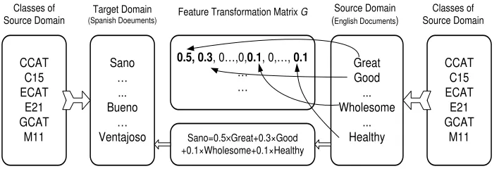
Figure 1: Illustration of the sparse feature representation matrix.
The above two assumptions are common in real-world multilingual text categorization appli-cations. Recall that the sparsity assumption of the feature mapping across domains implies that each feature in one domain can only be represented by a small subset of features in another do-main. Here, we still use the multi-language (i.e., English/Spanish) text classification problem as a motivating example. Typically, the word “Sano” in Spanish has a similar meaning to the words “Great”, “Good”, “Wholesome”, and “healthy” in English, but not to all English words. There-fore, by assuming that the feature mapping across domains is linear, a feature or word in the Spanish domain can be represented by a linear combination of only several features or words in the English domain. As illustrated in Figure 2.1, the sparse matrix G denotes the feature mapping from the English domain to the Spanish domain. Based on the sparse matrix G, the word “Sano” in Spanish can be represented sparsely by only four words in English as“Sano00 = 0.5דGreat00+ 0.3דGood00+ 0.1דWholesome00+ 0.1דHealthy00. This sparsity characteristic, which also facilitates a significant reduction in computational cost on very high-dimensional data, has not been explored in existing HDA methods. The feature mapping of the word “Sano” is invari-ant for different classes, for example, “CCAT” and “C15”. To encode theclass-invarianceproperty into the feature mapping, we propose to learn a common Gunderlying all the classes which has a similar spirit to multi-task feature learning (Argyriou et al., 2007) and domain-invariant feature learning (Gong et al., 2013). We first decompose a multi-class classification problem into multiple binary classification tasks, and then jointly optimize all the binary classification tasks and the feature mappingG, such thatGis class-invariant to all the binary classification tasks.
2.2 Our Contributions
1. We propose a Sparse Heterogeneous Feature Representation (SHFR) approach to learn a sparse transformation for HDA by exploring the common underlying structures between multiple classes.
2. Our major finding is that, based on the CS theory, a sparse feature mapping can be learned if and only if a sufficient number of classifiers are provided. Based on this analysis, we propose to generate sufficient classifiers under theError Correcting Output Correcting (ECOC) scheme to accurately estimate the sparse feature mapping.
3. To reduce the high computational cost, we propose a batch-modepursuit algorithm to ef-ficiently solve the resultant nonnegative lasso problem of SHFR. The computational cost of SHFR is independent of the data size and the dimensionality of the source domain data, and scales linearly only with size of the dimensionality of the target domain data.
4. This paper is the first to present ageneralization error boundfor multi-class HDA which is dependent on the number of tasks as well as the degree of sparsity of the feature mappingG.
The remainder of the paper is organized as follows. In Section 3, we first present how to for-mulate an HDA problem as a compressed sensing problem, and describe the detail of the proposed method, SHFR. We then theoretically analyze a generalization error bound for SHFR in Section 4, and develop a batch-mode algorithm in Section 5 to efficiently solve the resultant compressed sens-ing problem. In Section 6, we conduct extensive experiments on both toy and real-world datasets to demonstrate the effectiveness and efficiency of SHFR. We conclude this paper and discuss future work in Section 7.
3. Sparse Heterogeneous Feature Representation
We study the HDA problem with one source domain and one target domain under the multi-class setting. Let{(xSi, ySi)}
nS
i=1denote a set of labeled training instances of the source domain, where
xSi ∈R
dS denotes thei-th instance, andy
Si ∈ {1,2,· · · , c}denotes its label. Let{(xTi, yTi)}
nT
i=1
be a set of labeled training instances of the target domain, where nT nS, xTi ∈ R
dT, and
yTi ∈ {1,2,· · · , c}.
Given a binary taskt∈ {1,2,· · ·, nc}, we assume that the classifiers for both source and target domain are linear, which can be written asft(x) = wt>x, wherewtis the weight vector of the t-th classifier. Since there are sufficient labeled data in the source domain, i.e., {(xSi, ySi)}
nS
i=1,
we can learn a robust set of weight vectors{wtS}nc
t=1 for the source classifiers of the binary tasks
decomposed from the multi-class classification problem. Similarly, we can build a corresponding set of weight vectors{wtT}nc
t=1with limited labeled data{(xTi, yTi)}
nT
i=1for the target domain.
3.1 Feature Mapping for HDA
Recall that, for HDA problems, the feature dimensions of the source and target domains may not be equal, i.e., dS 6= dT. To make effective learning across heterogeneous domains possible, a transformation matrix G ∈ RdT×dS was introduced in ARC-t (Kulis et al., 2011; Saenko et al.,
2010) to learn the similarityx>TiGxSi between a source instancexSi ∈ R
dS and a target instance
xTi ∈ R
space viaxTi =GxSi, or equivalently, the target domain data can be mapped into the source
do-main via G> (Saenko et al., 2010). To learn the transformation matrix G, corresponding pairs across domains are usually supposed to be given in advance (Qi et al., 2011) or generated based on the label information in both the source and target domains (Saenko et al., 2010). However, in practice, instance-correspondences between domains are usually missing, or the constructed in-stance correspondences using label information are not precise. Therefore, instead of learning the transformation by using the input raw data directly, we adapt an idea from a multi-task learning method (Ando and Zhang, 2005)1, and propose to learn the feature mapping across heterogeneous features based on the source and target predictive structures, i.e.,{wtS}’s and{wtT}’s.
We can either learn the transformation matrixG∈RdT×dS by maximizing the dependency
be-tween the transformed weight vectors of source classifiers and the weight vectors of target classifiers via
max
G w
t> T GwSt,
or by minimizing the distance between these two vectors via
min
G kw
t
T −GwtSk.
For simplicity in theoretical analysis, we adopt the latter objective to learn the transformationG. Given a binary taskt∈ {1,· · ·, nc}and a transformationG ∈RdT×dS, the relationship between
the weight vectors of the source and target classifiers can be modeled as follows,
wTt −GwtS=w∆t ,
wherewt∆is referred to as a “delta” weight vector, and its`2-normkw∆t k2 is used to measure the
difference between the target weight vector wTt and the transformed source weight vectorGwtS. Note that the relationship is linear. This is because, in this paper, we focus on the application of HDA on cross-language text categorization, where using a linear form to model the relationship of predictive structures between domains is more suitable for high-dimensional text data. For modeling a nonlinear relationship between the source and target predictive structures, which may be more useful in other application areas, e.g., image classification or speech recognition, it is possible to apply an explicit nonlinear feature mappingφ(x)to both the source and target domain data before training the weight vectors for each domain.
3.2 Proposed Formulation
In order to use the robust source domain weight vectorwSt to make predictions on the target domain data, the difference between the source and target domains after transformation should be mini-mized. We therefore propose to learn the transformationGby minimizingkwt∆k2. As mentioned
in Section 2, the feature mappingGshould be class-invariant and sparse, and for multi-language text classification and many other real-world applications, the feature mappingGbetween feature spaces should be nonnegative. The motivation of adding the nonnegative constraint on the feature mappingGis similar to that of applying nonnegative matrix factorization (NMF) (Lee and Seung,
2001) to text mining. Here, we aim to approximate “input vectors”, i.e., target features, by a non-negative linear combination of a set of nonnon-negative “basis vectors”, i.e., source features, through the mappingG. This is also similar to multiple kernel learning (MKL) (Lanckriet et al., 2004; G¨onen and Alpaydın, 2011), where the target kernel is represented by the nonnegative linear combination of base kernels. In the context of multi-lingual text classification, the nonnegative entries inGcan be deemed as explicit “soft” global co-occurrences between the source and target wordbooks, while without the nonnegative constraint onG, it is difficult to interpret the physical or semantic meaning behindG.
LetG= [g1,g2,· · ·,gdT]
>, by imposing the`
1-regularization and the nonnegative constraint
on gi, the learning ofGcan be formulated as the following nonnegative LASSO problem (Yuan and Lin, 2007; Slawski and Hein, 2011),
min G 1 nc nc X t=1
kwtT −GwtSk22+
dT X
i
λikgik1, (1)
s.t. gi0,
whereλi >0is the trade-off parameter for the regularization term on eachgi. In (1), the first term in the objective aims to minimize the difference betweenwtT andGwtS over all the nc tasks, the second term in the objective is to enforce the sparsity on each row ofG, and the constraints are used to preserve nonnegative linear relations between the source and target predictive structures.
Note that in practice, once the source domain classifiers in terms of the weight vectors{wt S}
nc
t=1
are learned offline, the source domain training data can be discarded. For a new domain of interest, i.e., the target domain, the weight vectors{wTt}nc
t=1can first be learned with a few labeled training
data, and thenGcan be learned with{wt S}
nc
t=1instead of the original source domain training data,
which significantly reduces the learning complexity. This learning scheme is typically different from most of the existing HDA methods that require the original source domain training data to be available to learn the feature mapping across domains. More discussion on the complexity issue can be found in Section 5.1. AsGis learned through all the binary classification tasks, knowledge can be transferred from the easy tasks to the difficult ones. In Section 4.2, we theoretically show that as long as a significant number of base binary tasks are not badly designed, the generalization error of the target classification model is guaranteed to be small.
To solve the optimization problem (1), we can first rewrite it in the following equivalent form,
min gi 1 nc nc X t=1 dT X i=1
(wTti−wt>S gi)2+ dT X
i
λikgik1, (2)
s.t. gi 0,
wherewtTi is thei-th element of the vectorwtT. If we exchange the summation sequences in the first term, the above optimization problem can be reformulated as the following CS problem,
min gi dT X i 1 nc
kbi−Dgik22+λikgik1
, (3)
wherebi is the concatenated row vector containing{wTti}
nc
t=1, and D = [w1S wS2 · · · w nc
S ] > ∈
Rnc×dS.
This type of CS problem has been well studied, and a number of algorithms have been pro-posed to solve it, such as nonnegative least squares (NNLS) (Cantarella and Piatek, 2004), accel-erated proximal gradient algorithm (APG) (Toh and Yun, 2010), and orthogonal matching pursuit (OMP) (Zhang, 2009). In this work, we propose an efficient batch-mode algorithm to solve it, which is introduced in detail in Section 5. After the sparse transformationGhas been learned, we can reuse the source domain classifiers to predict its label for any unseen test datax∗T from the target domain via
y∗T =F({(GwtS)>x∗T}nc
t=1),
whereF(·)is a decision function that combines the predictive results of all thencsource classifiers to make a final prediction.
4. Generalization Error Bound for HDA
In the past decade, theoretical analysis for domain adaptation has been widely studied (Blitzer et al., 2007a; Mansour et al., 2009; Ben-David et al., 2010), and has focused on understanding conditions and assumptions of domain adaptation. However, most previous theoretical works were restricted by the assumption that the data from the source and target domains are represented in the same feature space and therefore cannot be applied directly to analyze the generalization error of our pro-posed method, SHFR, under the HDA setting. In this section, we analyze the theoretical guarantee of SHFR in detail. In contrast to existing generalization error analysis for homogeneous domain adaptation, we derive the generalization error bound for SHFR mainly from the perspectives of ECOC and compressed sensing.
4.1 Estimation Error Bound for Sparse Feature Mapping
Recall that the optimization problem (3) is composed ofdT lasso problems. In general, we have nc < dS for relatively high-dimensional data, therefore (3) is an underdetermined linear sys-tem (Donoho, 2006). However, based on the compressed sensing theory, if gi is sparse, it is possible to obtain a solution with sufficient measurements and a matrix D that satisfies certain conditions (Donoho, 2006; Cand`es et al., 2006). In particular, one such condition is the sparse Riesz condition or RIP condition, which requires that any two columns ofDshould be as perfectly incoherent as possible (Donoho, 2006; Zhang and Huang, 2008; Cand`es et al., 2006).
For simplicity in presentation, let ki denote the number of non-sparse entries of gi (or non-sparsity degree), andbgidenote an estimator ofgi. According to Theorem 3 and Remark 4 in (Zhang
and Huang, 2008), under some restricted conditions, the estimation error||gi −bgi||2 for each
in-dependent subproblem can be bounded byO
q
kilogdS
nc
, wheredSdenotes the dimensionality of the source domain data andncis the number of tasks. Hence, we can obtain the following lemma.
Lemma 1 Under the sparse Riesz condition, the estimation error k∆GCSkF = kG−GbkF in
(1) is bounded byOdT
q
klogdS
nc
Note that besides the sparse Riesz condition, Lemma 1 also holds under some other restricted con-ditions, such as the RIP condition (Zhang and Huang, 2008; Cand`es et al., 2006). Both the sparse Riesz condition and the RIP condition require that any two columns ofDshould be as incoherent as possible (Donoho, 2006; Zhang and Huang, 2008; Cand`es et al., 2006). However, although the RIP condition for randomly designed matrices has been thoroughly investigated (Baraniuk et al., 2008), it is more difficult to investigate it for deterministically designed matrices in general. In contrast, the sparse Riesz condition for a deterministically designed matrix holds with high probability if the following condition is satisfied (see Proposition 1 in (Zhang and Huang, 2008)):
max
|A|=kα≥inf1
X
j∈A
X
i∈A,i6=j
|ρji|α/(α−1)
α−1
1/α
≤δ <1,
wherekdenotes the non-sparsity degree andρji=d0jdi/nc.
Remark 2 Note thatρjican be deemed as the correlation between the columnsdj anddi.
There-fore, the sparse Riesz condition for a deterministically designed matrix can be evaluated by the correlations between the columns of the dictionary matrix. The smaller the summary of correla-tionsP
|ρji|(orδ) is, the more likely it is that the sparse Riesz condition forDwill hold.
According to Lemma 1 and Remark 2, to reduce the reconstruction error of the feature map-ping G, it is necessary to 1) construct as many classifiers as possible to increase the number of measurements, i.e.,ncneeds to be large enough, and 2) ensure the columns ofDconstructed from the classifiers are incoherent, i.e., D is incoherent. For a multi-class classification problem with labels{1,2,· · · , c}, cbinary classifiers can be generated using the one-vs-all strategy (Dietterich and Bakiri, 1995). However, when c is small, this strategy is not able to generate sufficient bi-nary classifiers. Alternatively, the one-vs-one strategy may be used to generatec(c−1)/2binary classifiers. The classifiers generated in this way may have large redundancy, however, i.e., some classifiers may be highly correlated to each other. To address this issue, we propose to use the Error Correcting Output Codes (ECOC) scheme (Dietterich and Bakiri, 1995; Zhou et al.) to generate sufficient binary classifiers for estimating the feature mappingG. As will be shown empirically in Section 6.5, greater incoherence forDover the one-vs-all or one-vs-one strategy can be guaranteed with a proper design of the ECOC coding matrix.
4.2 Generalization Error Analysis of HDA Based on ECOC
By using the ECOC scheme, the multi-class hypothesishis composed of a set of binary classifiers {Gwb tS}nt=1c . However, in contrast to the one-vs-all scheme, ECOC is more general and consists of
two steps: encoding, i.e., to design a coding matrixM to induce binary classifiers, and decoding, i.e., to combine the results of all the binary classifiers to make predictions based on the coding matrix. In order to analyze the generalization error bound of SHFR for multi-class HDA based on ECOC, we need to first analyze the principles of ECOC for multi-class classification.
As discussed in Dietterich and Bakiri (1995); Allwein et al. (2001), the prediction performance of a multi-class classification model learned based on the ECOC scheme depends on the design of the coding matrix. Given a coding matrixM = {−1,0,+1}c×nc, each class is associated with a
an entryM(i, j) = +1, it implies that in the classifierfj, classiis considered as a positive class, while ifM(i, j) = −1, it implies that in the classifier fj, the classiis considered as a negative class, otherwise, the class iis not taken into account for training and testing. In this way, either the one-vs-all scheme or the one-vs-one scheme can be considered as a special case of the ECOC scheme.
As pointed out by Dietterich and Bakiri (1995), a coding matrix is good if each codeword, i.e., each row, is well-separated in the Hamming distance from each of the other codewords, and each bit-position functionfk, i.e., each column, is uncorrelated with the functions to be learned for the other bit positionsfj,j 6= k. The power of a coding matrixM for multi-class classification can be measured by the minimum Hamming distance between any pair of its codewords (Allwein et al., 2001), denoted by∆min(M). For instance, for the one-vs-all code,∆min(M) = 2, and for the
one-vs-one code,∆min(M) =
c
2
−1
/2 + 1. For a random matrix with components chosen
over{−1,0,1}, the expected value of∆min(M)for any distinct pair of rows isnc/2.
Here, we first follow the proof procedure on error analysis for multi-class classification de-scribed in Allwein et al. (2001) to analyze the condition of a testing error by the ECOC decoding. After that, we derive the generalization error bound for the proposed SHFR with the ECOC scheme. Given a coding matrixM ∈ {−1,0,+1}c×nc, each row corresponds to a class and each column
corresponds to a binary task. For somet ∈ {1,2,· · · , nc}, we denote wtS andhtS as the source domain weight vector and the hypothesis of thet-th task defined by the coding matrixM, respec-tively. We denoteGwb tSandhtT as the estimated target domain weight vector and hypothesis of the
t-th task, respectively. We also define the loss function,
L(z) = (1−z)+= max{1−z,0}, (4)
in terms of the marginz. For example, given a target domain instancexTi with its labelyTi, the
corresponding marginzTt
ifort-th task is defined as
zTti =M(yTi, t)h
t
T(xTi) =M(yTi, t)((Gwb
t S)
>
xTi). (5)
For instance, SVM seeks to minimize the margin-based loss underL2 norm regularization as
fol-lows,
min w
1 2kwk
2 2+C
m
X
i=1
(1−yiw>xi)+, (6)
where we denote margin z = yiw>xi. When the prediction is correct and M(yTi, t) 6= 0 for
xTi, then the marginz
t
Ti > 0, which results in0 ≤ L(z) < 1; when the prediction is wrong and
M(yTi, t) 6= 0forxTi, then the marginz
t
Ti <0, which results inL(z) >1; whenM(yTi, t) = 0,
then the margin ztT
i = 0, which results inL(z) = 1. We define the L(z) loss-based decoding
scheme for prediction as follows:
dL(M(r,:), h(xTi)) =
nc X
t=1
L(M(r, t)htT(xTi)). (7)
To understand the error correction ability of ECOC, we first define the distance between the codes in any distinct pair of rows,M(r1,:)andM(r2,:), in the coding matrixM as
d(M(r1,:), M(r2,:)) =
nc X
s=1
d(M(r1, s), M(r2, s)), (8)
whered(M(r1, s), M(r2, s)) = 1−sign(M(r21,s)M(r2,s)).
We defineρ= minr16=r2d(M(r1,:), M(r2,:))as the minimum distance between any two rows
in the coding matrixM, which is pre-calculated before the training.
Proposition 3 Given a coding matrixM ∈ {−1,0,+1}c×nc, a set of hypothesis outputsh1(x),· · · , hnc(x) on a test instancexgenerated byncbase classifiers, and a convex loss functionL(z)in terms of
the marginz, ifxis misclassified by the loss-based ECOC decoding, then
nc X
t=1
L(M(y, t)ht(x))≥ρL(0), (9)
whereM(y, t)denotes the corresponding label generated by the coding matrixMof ground truth. In other words, the loss of the vector of predictionsf(x)is greater thanρL(0).
Proof Suppose that the loss-based ECOC decoding incorrectly classifies a test instancexwith the ground-truth labely. Then should then exist a labelr 6=ysuch that
dL(M(y,:), h(x))≥dL(M(r,:), h(x)).
By using the definitions of the loss function and margin introduced in (4) and (5), we denote
zt=M(y, t)ht(x),
z0t=M(r, t)ht(x), By using the definitions ofdLin (7), we have
nc X
t=1
L(zt)≥
nc X
t=1
L(z0t). (10)
LetS∆={t:M(r, t)6=M(y, t)∧M(r, t)6= 0∧M(y, t)6= 0}be the set of columns ofMwhose
r-th andy-th row entries are different and nonzero, and letS0 ={t:M(r, t) = 0∨M(y, t) = 0}
be the set of columns whoser-th ory-th row entry is zero. Ift /∈S∆∪S0, thenzt=z0t, and (10) implies that
X
t∈S∆∪S0
L(zt)≥ X
t∈S∆∪S0
L(z0t),
which, in turn, implies that nc X
t=1
L(zt)≥ X
t∈S∆∪S0
L(zt)
≥1
2 X
t∈S∆∪S0
(L(zt) +L(z0t))
=1 2
X
t∈S∆
(L(zt) +L(z0t)) + 1 2
X
t∈S0
Ift∈S∆, thenz0t=−ztand(L(−zt) +L(zt))/2≥L(0)due to convexity. Ift∈S0, then either
zt = 0orz0t= 0. Hence, we obtain thatL(z0t) +L(zt)≥L(0), and the second term of (11) is at leastL(0)|S0|/2. Therefore,
nc X
t=1
L(zt)≥1
2 X
t∈S∆
(L(zt) +L(z0t)) +1 2
X
t∈S0
(L(zt) +L(z0t))
≥L(0)
|S∆|+ |S0|
2
=L(0)d(M(r,:), M(y,:)) (12)
≥ρL(0),
where (12) is obtained from the fact that
d(M(r1, s), M(r2, s)) =
1−sign(M(r1, s)M(r2, s))
2 =
0 if M(r, t) =M(y, t)∧M(r, t)6= 0∧M(y, t)6= 0 1
2 if M(r, t) = 0∨M(y, t) = 0
1 if M(r, t)6=M(y, t)∧M(r, t)6= 0∧M(y, t)6= 0.
This completes the proof.
Remark 4 From Proposition 3, it can be seen that misclassification on a test instance(x, y)implies thatPnc
t=1L(M(y, t)ht(x)) ≥ρL(0). In other words, the prediction codes are not required to be exactly the same as ground-truth codes for all the base classifications. As long as the loss is smaller thanρL(0), ECOC can rectify the error committed by some base classifiers, and is still able to make an accurate prediction. This error-correcting ability is very important, especially when the labeled data is insufficient in the target domain. This proposition holds for any convex margin-based loss functionL(z). In this paper, we use hinge loss defined in (4), thenL(0) = 1.
Theorem 5 Letbe the averaged loss of the target domain hypothesesh1T, . . . , hnc
T on the target
test data{{(xTi, M(yTi, t))}
nT e
i=nT+1}
nc
t=1with respect to the coding matrixM ∈ {−1,0,+1}c×nc, wherecis the cardinality of the label set. Let the convex loss function beL(z) =|1−z|+. The multi-class HDA generalization error of SHFR using sparse random encoding and loss-based decoding is then at most nc
ρ .
Proof According to Proposition 3, the loss for any misclassified testing instancexT satisfies
ρL(0)≤
nc X
t=1
L(M(yT, t)htT(xT)).
Letabe the number of incorrect predictions for a test sample of sizenT e, then we can obtain the following inequality,
aρL(0)≤a nc X
t=1
L(M(yT, t)htT(xT))≤nT e nc X
t=1
Then we have
a≤ nT e
Pnc
t=1L(M(yT, t)htT(xT))
ρL(0) =
nT enc
ρ , (14)
where= Pnc
t=1L(M(yT,t)htT(xT))
nc andL(0) =|1−0|+= 1.
Therefore, the generalization error rate is bounded by nc
ρL(0). The proof is completed.
Remark 6 The above error bound is usually small in the setting studied in this paper for the fol-lowing reasons. When sufficient classifiers are generated using ECOC andGsatisfies the sparsity assumption, the reconstruction error is small and bounded according to the compressive sensing theory. On the other hand, the lossL(M(yT, t)htT(xT))for some{htT}s, which rely onG, may be
large due to there being limited target domain data. The data-independent termncis usually
pre-defined and the minimum distanceρ is determined correspondingly, asρmonotonically increases withncaccording to (8). Given the predefined ECOC coding matrix, as long as the averaged loss
is small, according to Theorem 5, target classifier is still able to make a precise prediction. In other words, SHFR is only unable to achieve satisfactory performance in terms of classification accuracy if most or all of the binary classifiers generated using ECOC trained on the target domain data are poorly designed.
In summary, we show that the multi-class HDA generalization error of SHFR based on the ECOC scheme has a linear relationship with the average loss over all generated binary classifiers when using random encoding and loss-based decoding methods. In addition to theoretical analy-sis, Garc´ıa-Pedrajas and Ortiz-Boyer (2011) conducted comprehensive experiments and concluded that ECOC and one-vs-one are superior to other multi-class classification schemes, and are the best choices for either powerful learners or simple learners. Furthermore, Montazer et al. (2012) claimed that, of several multi-class classification schemes, sparse ECOC is better than dense ECOC, while dense ECOC is better than one-vs-one, and one-vs-all is the worst. Ghani (2000) proved a theo-retical bound that a randomly-construct binary matrix is not well row-separated with probability at most1/c4, wherecis the number of classes. Therefore, in our experiments, we adopt the sparse and random ECOC scheme for multi-class HDA problems.
4.3 Robust Transformation Learning using ECOC
The robustness of ECOC is another important motivation for using ECOC in SHFR. Recall that the error-correcting codes can be viewed as a compact form of voting, and a certain number of incorrect votes can be corrected through the corrected votes (Dietterich and Bakiri, 1995). Given a total number ofT classifiers, the voting-based methods guarantee to make a correct decision as long as there arebT
2 + 1ccorrect classifiers (Dietterich, 2000), whereb cis thefloorfunction that returns
This property is particularly important for the proposed multi-class HDA method, SHFR, since some of the learned binary classifiers in the target domain may not be accurate due to insufficient label information. SHFR with ECOC is able to learn a robust transformation matrixGeven when some target binary classifiers are not precise. The robustness of SHFR with ECOC will be verified empirically in Section 6, where we demonstrate that even with inaccurate target classifiers, the class-invariant G learned by SHFR with the ECOC scheme can still dramatically enhance prediction accuracy for the target domain. By combining all the above theoretical analyses, we can conclude that the generalization error of our proposed method SHFR for multi-class HDA problems is small and bounded with a proper ECOC coding matrix design.
5. Efficient Batch Decoding for SHFR
In this section, we present an algorithm to solve the proposed optimization problem (3) of SHFR in detail. Recall that problem (3) containsdT LASSO problems with nonnegative constraints, which can be solved by adapting existing algorithms like NNLS solvers (Cantarella and Piatek, 2004; Slawski and Hein, 2011) or LASSO solvers, e.g., APG (Toh and Yun, 2010) and OMP (Zhang, 2009). However, the time complexity of these methods is O(ncdS) for each LASSO problem, which makes problem (3) intractable when the source domain data is of very high dimensionality and the number of LASSO problemsdT is very large.
Recall that each of the optimization problems (3) can be cast as the following problem
min
gi
1
nc
kbi−Dgik22+λikgik1, (15)
s.t. gi0,
wherebi ∈ Rnc×1 is the concatenated row vector containingwtTi for all the nc tasks, and D =
[w1S wS2 · · · wnc
S ] > ∈
Rnc×dS. For simplicity and without loss of clarity, we drop the subscripti
fromgiandbiin our discussion. Given anyg, let
ξ =b−Dg (16)
be the residual. Problem (15) can then be equivalently reformulated as the following problem
min
g0,ξ
λ||g||1+
1 2||ξ||
2, (17)
s.t. ξ =b−Dg.
Solving this problem directly can be very expensive when the source domain data is of very high dimensionality. Following Tan et al. (2015a), we propose to solve problem (15) via a matching pursuit method, called matching pursuit LASSO (MPL), as shown in Algorithm 1.
In Algorithm 1, the residualξ0 is initialized byξ0 =bsinceg0 =0. At thet-th step, we first
choose a set ofB components ing with theB largest values inD>ξt, and merge their indices Jt into the active setIt. We then solve a reduced problem whose scale is onlyO(nc|It|):
min
g0,ξ
λ||g||1+
1 2||ξ||
2, (18)
Algorithm 1Matching pursuit LASSO for solving the nonnegative LASSO problem.
Initialize the residualξ0 =b,I0 =∅, and lett= 1.
1: Computeq=D>ξt−1, choose theB largestqj, and record their indices byJt. 2: LetIt=It−1∪ Jt.
3: LetgIc
t =0, and solve the subproblem (18) to updategIt.
4: Computeξt=b−DgIt.
5: Terminate if the stopping condition is achieved. Otherwise, lett=t+ 1and go to step 1.
whereItdenotes the index set of the selected columns fromDandIc
t is the corresponding com-plementary set ofIt. This subproblem can be solved efficiently using a projected proximal gradient (PG) method. Note that the numberB in Step 1 is a small positive integer, e.g.,B = 1. Due to the nonnegative constraintsg 0, we find the elements with theB largest value inD>ξ rather than |D>ξ|.
Batch-mode MPL. In Algorithm 1, solving each subproblem has a complexity of O(knc), wherekdenotes the degree of the sparsity, namelyk=|It|, while computingD>ξhas a complexity ofO(dSnc). Note that problem (3) hasdT sub-problems as in (15). Therefore, computingD>ξ will dominate the whole complexity of the decoding if bothncanddT are very large.
To address the above computational burden imposed byD>ξ, we propose a batch-mode MPL (BMPL) algorithm. Note that D>ξ = D>(b−Dg) = D>b −D>Dg. We can pre-compute β = D>bandQ = D>D, and store them in the memory. SincegIc
t = 0for thet-th iteration,
we have D>ξt = D>b−[D>DIt]gIt = β−QItgIt, where QIt denotes the columns of Q
indexed byIt. The computation cost forD>ξis thus reduced toO(knc), which saves considerable computation cost whenk dS. Note thatβandQare shared by all the LASSO tasks, thus they only need to be calculated once. With this strategy, the overall computational cost of solving (3) whendSis large is significantly reduced toO(dTnck)(Tan et al., 2015a,b).
5.1 Complexity Comparison
We use linear SVMs to build the base classifiers for the source and target domains, which are ob-tained using the Liblinear solver (Fan et al., 2008) and pre-trained offline. The learning ofGis not related to the number of training instances. According to the analysis in Section 5, the computa-tional cost of SHFR isO(dTnck), where the sparsity degreekdS. Compared to state-of-the-art HDA methods, our proposed method is much more efficient. The MOMAP method transforms the problem intocseparate singular value decomposition (SVD) problems resulting in complexity of O(4d2SdT + 8dSd2T + 9d3T). The HeMap method is based on standard eigen-decomposition, whose complexity is O(nS +nT)3. The ARC-t method solves an optimization problem that contains nSnT constraints by applying an alternating projection method (e.g., Bregman’s algorithm (Censor and Zenios, 1997)), resulting in complexity ofdSdTnSnT. The HFA method adopts an alternating projection method to solve a semidefinite program (SDP), where the transformation matrix to be learned is in R(nS+nT)×(nS+nT), resulting in time complexity bounded byO(nS+nT)3. There-fore, ARC-t and HFA perform inefficiently when the data size is large. DAMA first constructs a series of combinatorial Laplacian matrices in R(dS+dT)×(dS+dT), and then solves a generalized
Table 1: Complexity comparison of HDA methods.
Methods Complexity
MOMAP (Harel and Mannor, 2011) O(4d2SdT + 8dSd2T + 9d3T) HeMap (Shi et al., 2010) O(nS+nT)3 DAMA (Wang and Mahadevan, 2011) O(dS+dT)3 ARC-t (Kulis et al., 2011) O(dSdTnSnT)
HFA (Duan et al., 2012) O(nS+nT)3 SHFR (our proposed method) O(dTnck)
computationally very expensive when the data dimensionality is high. The comparison in terms of time complexity between different methods is summarized in Table 1.
6. Experiments
In this section, we conduct experiments on both toy and real-world datasets to verify the effective-ness and efficiency of our proposed method SHFR for multi-class HDA. The parameter settings of our proposed method and other baseline methods are as follows. For ARC-t and HFA, which re-quire the use of kernel functions to measure data similarity, we use the RBF kernel for learning the transformation. Parameter tuning is still an open research issue, as cross-validation is not applicable to HDA problems due to the limited size of labeled data in the target domain. We therefore tune the parameters of the comparison methods on a predefined range and report their best results on the test data. We use linear SVMs as the base classifiers, the regularization parameterC of which is cross-validated from the range of{0.01,0.1,1,10,100}on the source domain data, and we use it for all the comparison methods. For our proposed method SHFR, we empirically set the maximum number of iterations to20,λ= 0.01andB = 2in the BGMP algorithm, and generate the ECOC as long as possible for each dataset.
6.1 Experiments on Synthetic Datasets
We first compare the performance of different HDA methods in terms of recovering a ground-truth feature mappingGon a 20-class toy dataset. To generate the toy dataset, we first randomly generate 150 instances of 150 features for each class from different Gaussian distributions to form a source domain XS ∈ R150×3,000. We then construct the ground-truth sparse feature mapping
G ∈ R100×150 using the following method: for each rowi, we setG
ij = 1/5, wherej = i, i+
1,· · · , i+ 5, andGij = 0otherwise. This generation ofGimplies that each target domain feature is represented by five source domain features. The ground-truth feature mapping is displayed in Figure 2(a), where the dark area represents the zero entries and the bright area denotes nonzero values ofG. Lastly, we construct the target domain dataXT ∈ R100×3,000 by usingXT =GXS.
When conducting the experiment, we randomly select five instances per class from the target domain dataXT as the labeled training data, and apply different HDA methods on them together with all 3,000 source domain labeled data to recover the feature mappingG.
(a) Ground Truth (b) DAMA
(c) ARC-t (d) SHFR
Figure 2: Illustration of the recovered feature mappings using different methods on the toy data. Black represents 0 and white represents 1.
shows better performance as can be seen in Figure 2(c). However, theGs recovered by these two methods are not sparse. In contrast, SHFR can perfectly recover the sparseGwith little noise as shown in Figure 2(d). These experimental results demonstrate that by explicitly adding sparsity constraints, SHFR is able to recover the feature mappingGmore accurately.
6.2 Experiments on Real-world Datasets
We conduct experiments on three real-world datasets, Multilingual Reuters Collection, BBC Col-lection, and Cross-lingual Sentiment Dataset, to verify the effectiveness and efficiency of SHFR. The reported results are averaged over 10 independent data-split procedures.
6.2.1 DATASETS AND EXPERIMENTALSETUP
Multilingual Reuters Collection2 is a text dataset with over 11,000 news articles from six cate-gories in five languages, i.e., English, French, German, Italian and Spanish, which are represented by a bag-of-words weighted by TF-IDF. Following the setting in Duan et al. (2012), we use Spanish as the target domain and the other four languages as source domains, which results in four multi-class HDA problems. For each multi-class, we randomly select 100 instances from the source domain
and 10 instances from the target domain for training. We randomly select 10,000 instances from the target domain as the test data. Note that the original data is of very high dimensionality, and the baseline methods cannot handle such high-dimensional features. To conduct comparison exper-iments, we first perform PCA with60%energy preserved on the TF-IDF features. We then obtain 1,131 features for the the English documents, 1,230 features for the French documents, 1,417 fea-tures for the German documents, 1,041 feafea-tures for the Italian documents, and 807 feafea-tures for the Spanish documents. In contrast to the baseline methods, we use original features for SHFR since it can efficiently handle high-dimensional data.
BBC Collection3 was collected for multi-view learning, and each instance is represented by three views. It was constructed from a single-view BBC corpora by splitting news articles into related “views” of text. We considerView 3as the target domain, andView 1andView 2as source domains. Similar to the pre-processing on the Reuters dataset, we perform PCA on the original data to reduce dimensions such that other baselines can be applied. The reduced dimensions forView 1,View 2andView 3are 203, 205 and 418, respectively. We randomly select70%source domain instances and 10 target domain instances for each class for training. The remaining target domain instances are considered to be the test data.
Cross-lingual Sentiment Dataset4 consists of Amazon product reviews of three product cate-gories: books, DVDs and music. These reviews are written in four languages: English, German, French, and Japanese. We treat English reviews as the source domain data and the other language reviews as the target data domain data. After performing PCA, the reviews are of 715, 929, 964, and 874 features for English, German, French and Japanese, respectively. We randomly select 1,500 source domain instances and 10 target domain instances per class for training, and use the rest 5,970 target domain instances for testing.
6.2.2 OVERALLCOMPARISONRESULTS
Comparison results between SHFR and other baselines on the three real-world datasets are reported in Tables 2-4. From the tables, we observe that the SVMs conducted on a small number of target domain data only, denoted by SVM-T, using either one-vs-one or one-vs-all strategy, perform the worst on average. Moreover, the results of SVM-T using one-vs-one and one-vs-all, respectively, are not consistent. For instance, on the BBC dataset in Table 3, SVM-T using the one-vs-all strategy performs much better than SVM-T using the one-vs-one strategy, while on the sentiment dataset in Table 4, SVM-T using the vs-one strategy performs much better than SVM-T using the one-vs-all strategy. The reason is that the size of the labeled training data is too limited to train a precise and stable classifier in the target domain. Compared to one-vs-all and one-vs-one, SVM-T with ECOC shows much more stable performance and superior results on most problems, which is because of the error correcting ability of ECOC when the labeled data is limited. The performance in terms of classification accuracy of the HDA baseline methods, DAMA, ARC-t and HFA, are comparable on the three datasets except for the BBC dataset, where DAMA performs much worse than the other two methods. This may be because the performance of DAMA is sensitive to the intrinsic manifold structure of the data. If the manifold assumption does not hold on the data, the performance of DAMA drops significantly. Our proposed SHFR method using either the one-vs-one or ECOC scheme performs best on the three datasets. SHFR can further improve the performance
3. http://mlg.ucd.ie/datasets/segment.html
Table 2: Multilingual Reuters Collection: comparison results in terms of classification acc (%). Results of SHFR are significantly better than the other baselines, judged by the t-test with a significance level at 0.05.
Source SVM-T SVM-T SVM-T DAMA ARC-t HFA SHFR SHFR
Domain (1 vs all) (1 vs 1) (ECOC) (1vs1) (ECOC)
English
65.40±4.45 65.21±7.85 68.01±2.48
63.42±2.62 66.72±2.27 68.82±1.68 69.45±1.56 72.82±1.08
French 65.12±1.28 67.67±2.05 68.14±1.71 70.77±1.57 74.01±1.25
German 66.98±2.45 68.15±1.72 68.42±1.57 71.62±1.69 74.15±1.14
Italian 67.56±2.23 67.47±2.32 69.59±2.51 70.75±1.54 73.35±1.31
Table 3: BBC Collection: comparison results in terms of classification acc (%). Results of SHFR are significantly better than the other baselines, judged by the t-test with a significance level at 0.05.
Source SVM-T SVM-T SVM-T DAMA ARC-t HFA SHFR SHFR
Domain (1 vs all) (1 vs 1) (ECOC) (1vs1) (ECOC)
View 1
73.35±4.98 68.78±11.7 76.45±5.47 67.42±2.25 75.78±2.69 72.45±10.65 89.81±1.20 90.57±1.49 View 2 66.87±1.73 74.53±2.48 73.75±8.06 88.92±1.67 91.85±0.96
Table 4: Cross-lingual Sentiment Dataset: comparison results in terms of classification acc. (%). Results of SHFR are significantly better than the other baselines, judged by the t-test with a significance level at 0.05.
Target SVM-T SVM-T SVM-T DAMA ARC-t HFA SHFR SHFR
Domain (1 vs all) (1 vs 1) (ECOC) (1vs1) (ECOC)
French 48.40±3.45 58.30±5.01 57.45±3.17 55.18±3.46 53.46±5.18 56.46±3.42 60.80±3.08 62.12±2.61
German 49.78±5.12 61.62±6.31 62.18±4.51 56.60±3.72 57.29±2.17 55.14±3.15 63.85±3.46 65.57±2.32
Japanese 48.25±6.34 56.13±4.81 57.27±2.61 53.56±2.67 55.75±3.02 55.02±4.67 59.67±3.75 62.58±2.86
in terms of classification accuracy, compared to one-vs-one, using the ECOC scheme. The superior performance benefits from both the global transformation ofGand the error correcting ability of ECOC. As discussed in Section 4.1, the recovered feature mapping Gtends to be more accurate with more constructed binary tasks.
6.3 Impact on Training Sample Size of the Target Domain
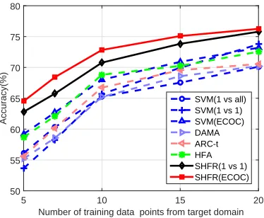
We verify the impact of the size of labeled training sample in the target domain to the overall HDA performance in terms of classification accuracy. We vary the number of target domain training instances from five to 20. In this experiment, we only report the results on the Reuters dataset, where we use English as the source domain and Spanish as the target domain. The experimental results are shown in Figure 3. From the figure, we observe that SHFR consistently outperforms the baseline methods under different numbers of labeled training instance in the target domain. In particular, SHFR shows significantly better performance than the baseline methods when the size of the target domain labeled data is smaller than 10.
Number of training data points from target domain
5 10 15 20
Accuracy(%)
50 55 60 65 70 75 80
SVM(1 vs all) SVM(1 vs 1) SVM(ECOC) DAMA ARC-t HFA SHFR(1 vs 1) SHFR(ECOC)
Figure 3: Comparison of different HDA methods under varying size of target labeled data.
5 10 15 20
66 68 70 72 74 76 78 80 82 84
Target binary SVMs accuracy (%)
Number of labeled target data points
(a) Averaged binary accuracy v.s. target data size.
65 70 75 80 85 60
62 64 66 68 70 72 74 76 78
Multi−class SHFR accuracy (%)
Target binary SVMs accuracy (%)
(b) Multiclass accuracy v.s. averaged binary accuracy.
Figure 4: Relationships between binary base classifiers and multi-class SHFR (ECOC).
averaged accuracy of all binary classifiers generated based on ECOC on the Reuters dataset under varying numbers of labeled training instances in the target domain in Figure 4(a). We also report the overall multi-class prediction accuracy versus the averaged accuracy of all binary classifiers in Figure 4(b). From the figures, we see that more labeled target data leads to more precise target binary classifiers, and thus leads to improvement in multi-class HDA classification in terms of accuracy. In particular, we observe from Figure 4(b) that the multi-class classification accuracy is proportional to the averaged binary task accuracy. The reason is that more precise target binary classifiers generally induce better alignment between the target and source classifiers.
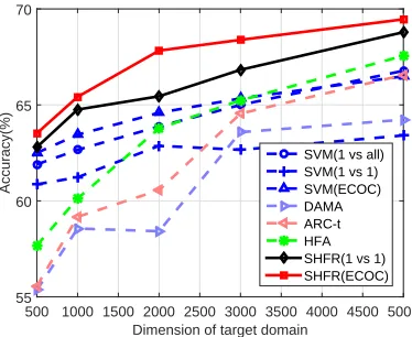
6.4 Impact on Dimensionality of the Target Domain
Dimension of target domain
500 1000 1500 2000 2500 3000 3500 4000 4500 5000
Accuracy(%)
55 60 65 70
SVM(1 vs all) SVM(1 vs 1) SVM(ECOC) DAMA ARC-t HFA SHFR(1 vs 1) SHFR(ECOC)
Figure 5: Comparison of different HDA methods under varying dimensions of target labeled data.
Table 5: Comparison in correlationP
ji|ρji|.
Coding Scheme English French German Italian
1 vs all 0.8532±0.1358 0.7557±0.1289 0.2738±0.0245 0.9331±0.5701 1 vs 1 0.3374±0.0290 0.2509±0.0576 0.1168±0.0110 0.3322±0.1679 ECOC 0.1349±0.0142 0.1478±0.0225 0.0732±0.0145 0.1725±0.1047
the target domain, in the range of {500,1000,2000,3000,5000} by selecting the most-frequent features of this domain. The results are shown in the Figure 5, from which we observe that SHFR consistently outperforms other baselines, especially when the dimensionality of the target domain data is low.
6.5 Incoherent DictionaryDConstruction
In this experiment, we adopt the summation of absolute value of all pairs of columns in the dictio-naryD to evaluateD’s coherence degree, i.e., P
ji|ρji|. In other words, the smaller the value of
P
ji|ρji|is, the more incoherent the dictionary is (Zhang and Huang, 2008). The results of different coding schemes on the Reuters dataset are summarized in Table 5. From the table, we observe that ECOC can be used to significantly reduce the coherence degree to enable better construction of the dictionary for the formulated compressed sensing problem.
6.6 Error Correction through Learning a GlobalG
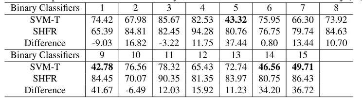
Table 6: Comparison results on each binary task in terms of classification accuracy (%).
Binary Classifiers 1 2 3 4 5 6 7 8
SVM-T 74.42 67.98 85.67 82.53 43.32 75.95 66.30 73.92 SHFR 65.39 84.81 82.45 94.28 80.76 76.75 79.74 84.63 Difference -9.03 16.82 -3.22 11.75 37.44 0.80 13.44 10.70
Binary Classifiers 9 10 11 12 13 14 15
SVM-T 42.78 76.56 78.32 65.43 72.74 46.56 49.71 SHFR 84.45 70.07 90.35 81.35 83.97 80.75 86.43 Difference 41.67 -6.49 12.03 15.92 11.23 34.20 36.72
and increase accuracy by more than30%on average. Experiments on the other two datasets return similar results, where the performance in terms of accuracy of the binary classifiers obtained through G is increased by26.53% on the BBC dataset and3.01% on the Sentiment dataset on average, compared to the results generated by SVM-T.
The experimental results in Table 6 also verify why SHFR outperforms ARC-t in the experi-ments shown in Tables 2-4 and Figure 3. ARC-t aims to align the target data with the source data via a transformationGthat is learned from similarity and dissimilarity constraints. The constraints are constructed from a large number of source domain labeled data and a few target domain labeled data. In the multi-class setting, the number of similarity constraints to be constructed when the number of classes is large is much smaller than the number of dissimilarity constraints due to the limited number of target domain labeled data. In contrast to ARC-t, SHFR tries to align the target classifiers with the source classifiers using transformation G, which is shared by all the induced binary tasks or classifiers. In other words, Gis estimated through all classifiers. By borrowing the idea from multi-task feature learning which jointly optimizes all classifiers to learn a global feature transformationG, is still possible to estimate a stable and preciseGfor multi-class HDA. Furthermore, as discussed in Section 4.3, ECOC with a well designed coding matrix is powerful for correcting error, as shown in Table 6.
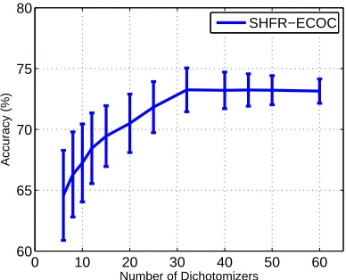
6.7 Impact of Dichotomizer Size on Classification Error
As proven in Section 4, the generalization error of SHFR for multi-class HDA depends on the averaged loss over all the tasks, which relies on two factors: the number of classifiers (or measure-ments) and the degree of sparsity on G. When Gis sparse and the constructed binary classifiers are sufficient, it is possible to recover a preciseGby using the dictionary constructed bywS. To demonstrate how the generalization error of SHFR changes under varying numbers of classifiers or dichotomizers, we conduct experiments on the Reuters dataset.
bet-0 10 20 30 40 50 60 60
65 70 75 80
Number of Dichotomizers
Accuracy (%)
SHFR−ECOC
Figure 6: Accuracy vs dichotomizer (or task) size.
Table 7: Impact of Nonnegative Constraints andL1Norm Regularization: comparison between the
results of different solvers in terms of classification accuracy (%). Results of SHFR are significantly better than the other baselines except for the cases denoted with *, judged by the t-test with a significance level at 0.05.
Dataset Domain SHFR-LASSO SHFR-NNLS SHFR
Reuters
English 67.08±1.63 71.47±1.56 72.82±1.08 French 67.17±1.26 72.08±1.19 74.01±1.25 German 69.56±1.28 73.62±1.75* 74.15±1.14 Italian 68.19±2.51 71.98±1.78 73.35±1.31
BBC View 1 84.72±2.18 88.66±1.29 90.57±1.49 View 2 87.06±2.01 90.25±1.43 91.85±0.96
Sentiment
French 56.12±2.30 60.17±2.05 62.12±2.61 German 58.83±2.24 63.47±1.49 65.57±2.32 Japanese 56.72±1.81 61.51±1.76* 62.58±2.86
ter and more stable performance in terms of classification accuracy with an increasing number of dichotomizers.
6.8 Impacts of Nonnegative Constraints and`1Norm Regularization
Regarding the`1norm regularization term in SHFR, note that some studies in the literature have
shown that Non-Negative Least Squares (NNLS) can indeed achieve sparse recovery of nonnega-tive signals in a noiseless setting (Bruckstein et al., 2008; Donoho and Tanner, 2010; Wang and Tang, 2009; Wang et al., 2011). However, the noiseless assumption does not hold in practice. As mentioned by Slawski et al. (2013), apart from sign constraints, NNLS only consists of a fitting term, and thus is prone to overfitting, especially when the training data is high-dimensional. The `1-norm regularizer is therefore necessary to prevent over-adaptation to noisy data and enforce
de-sired structural properties of the solution, which is similar to the idea of adding sparsity to the vector of coefficients of a predictive model (Slawski et al., 2013). In our proposed optimization problem (1), it is insufficient to achieve desirable solution ofGwithout the`1-norm term in the objective
since bothwtSandwtT are of high dimensionality, and some of{wtT}’s are not precise. As stated in Theorem 1 in Slawski and Hein (2011), exact sparsity, i.e.,`1-norm, is not needed when the matrix
satisfies the self-regularizing property, which is not applicable to our optimization problem asG does not have this property. Using the`1-norm ensures that a more sparse solution can be achieved
by using nonnegative constraints. To verify the impact of the`1-norm onG, we add another
base-line for comparison by moving the`1-norm from the the optimization problem of SHFR, which is
denoted by SHFR-NNLS. In this case, the model is reduced to an NNLS problem. In this paper, we adopt the NNLS solver proposed by Cantarella and Piatek (2004) to solve it.5
The results on the three multilingual datasets are summarized in Table 7. We observe from the table that SHFR-LASSO performs the worst and SHFR-NNLS enhances its performances through the nonnegative constraint. This is probably because the feature mapping G is learned globally and the features are naturally nonnegative for text classification. As SHFR explicitly imposes both nonnegativity and sparsity in learning the transformationG, it can further enhance the performance compared to SHFR-NNLS by avoiding over adapting the noise in the high-dimensional data.
6.9 Experiments on Removing Negative Alignment
We have observed from Table 6 that the accuracy of SHFR for some constructed binary tasks is slightly less than the accuracy of SVM-T after learning and using the transformationG, which can be referred to asnegative transfer(Pan and Yang, 2010). The problem of negative transfer in SHFR mainly occurs for the following two reasons:
1. Negative alignmentbetween the source and target classifiers, which happens when the clas-sification accuracy of the corresponding target classifier is below50%. This is because some initial target classifiers are less accurate due to the limited number of target domain labeled data.
2. The transformation Gis class-invariant, therefore G is enforced to generalize well on all classifiers. In this case,Gmay correct the bias of some weak classifiers, but may also smooth the strength of good classifiers.
In this experiment, we study how the performance of SHFR is affected by removing negative alignments, and how SHFR performs if only good target classifiers whose accuracy is above50%
Table 8: Comparison results on each binary task after removing negative alignment in terms of classification accuracy (%).
Binary Classifiers 1 2 3 4 5 6 7 8
SVM-T 74.42 67.98 85.67 82.53 43.32 75.95 66.30 73.92 SHFR-RN 85.39 83.26 86.45 92.43 83.79 78.19 77.45 81.28 Difference 10.97 15.28 0.87 9.90 40.47 2.24 11.15 7.36
Binary Classifiers 9 10 11 12 13 14 15
SVM-T 42.78 76.56 78.32 65.43 72.74 46.56 49.71 SHFR-RN 84.15 78.45 92.14 82.12 84.58 82.72 88.61 Difference 41.37 1.89 13.82 16.69 11.84 36.16 38.90
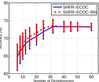
are used. We investigate whether dropping negative alignments improves accuracy on all the binary tasks as well as the final multi-class HDA classification problem. Experimental results are shown in Table 8 and Figure 7. Compared to the results in Table 6, we discover from Table 8 that by removing the negative alignments we can improve all binary classification performances in terms of accuracy, and thus avoid negative transfers. We sort the binary tasks created from ECOC according to the ac-curacy on the test data and remove the poorly designed tasks. From Figure 7, we observe that when the number of dichotomizers is small (e.g., less than 30), SHFR with negative alignment removed achieves better performance in terms of multi-class classification accuracy. However, in practice, it is difficult to evaluate target classifiers due to the limit number of target domain labeled data. Inter-estingly, we can also find from Figure 7 that when the number of dichotomizers or tasks is sufficient, the classification accuracy of SHFR with or without removing negative alignments converges to the same value. This is because sub-class partition in ECOC often leads to higher binary accuracy when creating many dichotomizers or tasks. In this case, there are fewer binary target classifiers whose accuracy is below 50%. Therefore, we can conclude that SHFR with negative alignments removed enhances the performance in terms of classification accuracy when there are insufficient classifiers. In the multi-class HDA setting, however, the difficulty in alignment evaluation makes this post-processing impractical. Fortunately, SHFR can achieve the same performance as SHFR-RNs when there are sufficient dichotomizers or tasks, which makes SHFR more practicable for the multi-class HDA problem.
6.10 Training Time Comparison
0 10 20 30 40 50 60 60
65 70 75 80
Number of Dichotomizers
Accuracy (%)
SHFR−ECOC SHFR−ECOC−RN
Figure 7: Accuracy v.s. dichotomizers size on removing tasks with negative alignment.
Dimension of training data
102 103 104
Training time(seconds)
0 1000 2000 3000 4000 5000 6000 7000 8000
DAMA ARC-t HFA SHFR
(a) Training time v.s. data dimensions
Number of training data
102 103 104
Training time(seconds)
100 101 102 103 104
DAMA ARC-t HFA SHFR
(b) Training time v.s. data size
Figure 8: Time complexity comparison
is because these two methods adopt the kernel technique such that the computational time depends on the number of data instances instead of the data dimensions. In the second experiment, shown in Figure 8(b), we fix the data dimension to 1,000 and vary the number of training instances in the range of{100,500,1000,2000,5000}. From the figure, we observe that the training time of SHFR changes slightly when the number of training instances increases. However, the training time of ARC-t and HFA increases polynomially when the number of training instances increases. These two experiments verify the superiority of SHFR in computational efficiency compared with the baseline methods.
7. Conclusion and Future Work
HDA. SHFR encodes the sparsity and class-invariance properties in learning the feature mapping. Learning feature mapping can be cast as a Compressed Sensing (CS) problem for SHFR. Based on the CS theory, we show that the number of binary learning tasks affects the multi-class HDA per-formance. In addition, the proposed method has superior scalability over other methods. Extensive experiments demonstrate the effectiveness, efficiency, and stability of SHFR.
In future, we would like to investigate how to extend the proposed method by exploring the nonlinear feature transformation between image and text feature representations.
Acknowledgments
We would like to thank the action editor Shie Mannor and anonymous reviewers for their valuable comments and constructive suggestions that greatly contributed to improving the final version of the paper.
Joey Tianyi Zhou was partially supported by programmatic grant no. A1687b0033, A18A1b0045 from the Singapore government’s Research, Innovation and Enterprise 2020 plan (Advanced Man-ufacturing and Engineering domain). Ivor W. Tsang acknowledges the partial funding from the ARC Future Fellowship FT130100746, ARC grant LP150100671, and DP180100106. Sinno J. Pan thanks the support from NTU Singapore Nanyang Assistant Professorship (NAP) grant M4081532.020, Singapore MOE AcRF Tier-2 grant MOE2016-T2-2-060, and the Data Science & Artificial Intelli-gence Research Centre at NTU Singapore. Mingkui Tan was partially supported by National Natural Science Foundation of China (NSFC) 61602185, Program for Guangdong Introducing Innovative and Enterpreneurial Teams 2017ZT07X183, Guangdong Provincial Scientific and Technological Funds under Grants 2018B010107001.
References
Erin L. Allwein, Robert E. Schapire, and Yoram Singer. Reducing multiclass to binary: A unifying approach for margin classifiers. J. Mach. Learn. Res., 1:113–141, September 2001.
Rie K. Ando and Tong Zhang. A framework for learning predictive structures from multiple tasks and unlabeled data. J. Mach. Learn. Res., 6:1817–1853, 2005.
Andreas Argyriou, Theodoros Evgeniou, and Massimiliano Pontil. Multi-task feature learning. In
NIPS, pages 41–048. MIT Press, 2007.
Richard Baraniuk, Mark Davenport, Ronald DeVore, and Michael Wakin. A simple proof of the restricted isometry property for random matrices. Constr. Approx., 28(3):253–263, 2008.
Shai Ben-David, John Blitzer, Koby Crammer, and Fernando Pereira. Analysis of representations for domain adaptation. InNIPS, pages 137–144, 2006.
Shai Ben-David, John Blitzer, Koby Crammer, Alex Kulesza, Fernando Pereira, and Jennifer Wort-man Vaughan. A theory of learning from different domains. Mach. Learn., 79(1-2):151–175, May 2010.
John Blitzer, Koby Crammer, Alex Kulesza, Fernando Pereira, and Jennifer Wortman. Learning bounds for domain adaptation. InNIPS, 2007a.
John Blitzer, Mark Dredze, and Fernando Pereira. Biographies, bollywood, boom-boxes and blenders: Domain adaptation for sentiment classification. InACL, 2007b.
Alfred M Bruckstein, Michael Elad, and Michael Zibulevsky. On the uniqueness of nonnegative sparse solutions to underdetermined systems of equations. IEEE Trans. Inform. Theory, 54(11): 4813–4820, 2008.
Emmanuel J. Cand`es, Justin K. Romberg, and Terence Tao. Stable signal recovery from incomplete and inaccurate measurements. Comm. Pure Appl. Math., 59(8):1207–1223, August 2006.
Jason Cantarella and Michael Piatek. TSNNLS: A solver for large sparse least squares problems with non-negative variables. arXiv preprint cs/0408029, 2004.
Yair Censor and Stavros A. Zenios. Parallel Optimization: Theory, Algorithms and Applications. Oxford University Press, 1997.
Wenyuan Dai, Yuqiang Chen, Gui-Rong Xue, Qiang Yang, and Yong Yu. Translated learning: Transfer learning across different feature spaces. InNIPS, pages 353–360, 2008.
Hal Daum´e III. Frustratingly easy domain adaptation. InACL, pages 256–263. ACL, June 2007.
Thomas G. Dietterich. Ensemble methods in machine learning. In MCS, pages 1–15. Springer-Verlag, 2000.
Thomas G. Dietterich and Ghulum Bakiri. Solving multiclass learning problems via error-correcting output codes. J. Artif. Intell. Res., 2:263–286, 1995.
Jeff Donahue, Judy Hoffman, Erik Rodner, Kate Saenko, and Trevor Darrell. Semi-supervised domain adaptation with instance constraints. InCVPR, 2013.
David L. Donoho. Compressed sensing. IEEE Trans. Inform. Theory, 52:1289–1306, 2006.
David L Donoho and Jared Tanner. Counting the faces of randomly-projected hypercubes and orthants, with applications. Discrete & Comput. Geom., 43(3):522–541, 2010.
Lixin Duan, Ivor W. Tsang, Dong Xu, and Tat-Seng Chua. Domain adaptation from multiple sources via auxiliary classifiers. InICML, pages 289–296, 2009.
Lixin Duan, Dong Xu, and Ivor W. Tsang. Learning with augmented features for heterogeneous domain adaptation. InICML, 2012.
Rong-En Fan, Kai-Wei Chang, Cho-Jui Hsieh, Xiang-Rui Wang, and Chih-Jen Lin. LIBLINEAR: A library for large linear classification. J. Mach. Learn. Res., 9:1871–1874, 2008.
Nicol´as Garc´ıa-Pedrajas and Domingo Ortiz-Boyer. An empirical study of binary classifier fusion methods for multiclass classification. Inf. Fusion, 12(2):111–130, April 2011.