The Thirty-Third AAAI Conference on Artificial Intelligence (AAAI-19)
Lifted Proximal Operator Machines
Jia Li, Cong Fang, Zhouchen Lin
∗Key Laboratory of Machine Perception (MOE), School of EECS, Peking University, P. R. China [email protected]; [email protected]; [email protected]
Abstract
We propose a new optimization method for training feed-forward neural networks. By rewriting the activation function as an equivalent proximal operator, we approximate a feed-forward neural network by adding the proximal operators to the objective function as penalties, hence we call the lifted proximal operator machine (LPOM). LPOM isblock multi-convexin all layer-wise weights and activations. This allows us to use block coordinate descent to update the layer-wise weights and activations. Most notably, we only use the map-ping of the activation functionitself, rather than its derivative, thus avoiding the gradient vanishing or blow-up issues in gra-dient based training methods. So our method is applicable to various non-decreasing Lipschitz continuous activation func-tions, whichcan be saturating and non-differentiable. LPOM does not require more auxiliary variables than the layer-wise activations, thus using roughly the same amount of memory as stochastic gradient descent (SGD) does. Its parameter tuning is also much simpler. We further prove the convergence of updating the layer-wise weights and activations and point out that the optimization could be made parallel by asynchronous update. Experiments on MNIST and CIFAR-10 datasets testify to the advantages of LPOM.
Introduction
Feed-forward deep neural networks (DNNs) are cascades of fully connected layers and there are no feedback connections. In recent years, with the advances in hardware and dataset sizes, feed-forward DNNs have become standard in many tasks, such as image recognition (Krizhevsky, Sutskever, and Hinton 2012), speech recognition (Hinton et al. 2012), natural language understanding (Collobert et al. 2011), and building the Go game learning system (Silver et al. 2016).
For several decades, training a DNN is accomplished by optimizing a highly nonconvex and nested function of the net-work weights. The predominant method for training DNNs is stochastic gradient descent (SGD) (Rumelhart, Hinton, and Williams 1986), whose effectiveness has been demonstrated by the successes of DNNs in various real-world applications. Recently, many variants of SGD have been proposed, which use adaptive learning rates and momentum terms, e.g., Nes-terov momentum (Sutskever et al. 2013), AdaGrad (Duchi,
∗
Corresponding author.
Copyright c2019, Association for the Advancement of Artificial Intelligence (www.aaai.org). All rights reserved.
Hazan, and Singer 2011), RMSProp (Dauphin, de Vries, and Bengio 2015), and Adam (Kingma and Ba 2014). SGD and its variants use a few training samples to estimate the full gra-dient, making the computational complexity of each iteration small. Moreover, the estimated gradients have noise, which is helpful for escaping saddle points (Ge et al. 2015). However, they have some drawbacks as well. One major problem is the vanishing or blow-up gradient issue, where the magnitudes of gradients decrease or increase exponentially with the number of layers. This causes slow or unstable convergence, espe-cially in very deep networks. This flaw can be remitted by using non-saturating activation functions, such as rectified linear unit (ReLU), and modified network architectures, such as ResNet (He et al. 2016). However, the fundamental prob-lem remains. Also, their parameters are difficult to tune (e.g., learning rates and convergence criteria) (Le et al. 2011). Fur-thermore, they cannot deal with non-differentiable activation functions directly (e.g., binarized neural networks (Hubara et al. 2016)) and do not allow parallel weight updates across the layers (Le et al. 2011). For more on the limitations of SGD, please refer to (Taylor et al. 2016) and (Le et al. 2011).
activa-tion funcactiva-tion is equivalent to a simple constrained convex minimization problem, Zhang and Brand (2017) relaxed the nonlinear constraints as penalties, which encode the network architecture and the ReLU activation function. Thus, the non-linear constraints no longer exist. However, their approach is limited to the ReLU function and does not apply to other activation functions. Askari et al. (2018) followed this idea by considering more complex convex optimization problems and discussed several types of non-decreasing activation func-tions. However, their methods to update the weights and acti-vations are still limited to the ReLU function. Their approach cannot outperform SGD and can only serve for initializing SGD. Actually, we have found that their formulation was incorrect (see Subsection “Advantages of LPOM”).
This paper makes the following contributions:
• We propose a new formulation to train feed-forward DNNs, which we call the lifted proximal operator machine (LPOM)1. LPOM is block multi-convex, i.e., the problem
is convex w.r.t. weights or activations of each layer when the remaining weights and activations are fixed. In contrast, almost all existing DNN training methods do not have such a property. This greatly facilitates the training of DNNs.
• Accordingly, we apply block coordinate descent (BCD) to solve LPOM. Most notably, the update of the layer-wise weights or activations only utilizes the activation function itself, rather than its derivative, thus avoiding the gradient vanishing or blow-up issues in gradient based training methods. Moreover, LPOM does not need more auxiliary variables than the layer-wise activations, thus its memory cost is close to that of SGD. It is also easy to tune the penalties in LPOM. We further prove that the iterations to update layer-wise weights or activations are convergent.
• Since only the activation function itself is involved in com-putation, LPOM is able to handle general non-decreasing Lipschitz continuous activation functions, which can be sat-urating (such as sigmoid and tanh) and non-differentiable (such as ReLU and leaky ReLU). So LPOM successfully overcomes the computational difficulties when using most of existing activation functions.
We implement LPOM on fully connected DNNs and test it on benchmark datasets, MNIST and CIFAR-10, and obtain sat-isfactory results. For convolutional neural networks (CNNs), since we have not reformulated pooling and skip-connections, we leave the implementation of LPOM on CNNs to fu-ture work. Note that the existing non-gradient based ap-proaches also focus on fully connected DNNs first (Carreira-Perpinan and Wang 2014; Zeng et al. 2018; Taylor et al. 2016; Zhang, Chen, and Saligrama 2016; Zhang and Brand 2017; Askari et al. 2018). We also point out that LPOM could be solved in parallel by asynchronous update.
Related Work
The optimization problem for training a standard feed-forward neural network is:
min
{Wi}` φ(W
n−1φ(· · ·φ(W2φ(W1X1))· · ·)), L , (1) 1
Two patents were filed in Nov. 2017 and Oct. 2018, respectively.
whereX1 ∈ Rn1×mis a batch of training samples, L ∈
Rc×mdenotes the corresponding labels,n1is the dimension of the training samples,mis the batch size,cis the number of classes,{Wi}n−1
i=1 are the weights to be learned in which the biases have been omitted for simplicity,φ(·)is an element-wise activation function (e.g., sigmoid, tanh, and ReLU), and `(·,·)is the loss function (e.g., the least-square error or the cross-entropy error). Here the neural network is defined as a nested function, where the first layer function of the neural network isφ(W1X1), thei-th layer (i= 2,· · · , n) function has the formφ(WiX), andX is the output of the(i−1) -th layer function. A common approach to optimize (1) is by SGD, i.e., calculating the gradient w.r.t. all weights of the network using backpropagation and then updating the weights by gradient descent.
By introducing the layer-wise activations as a block of auxiliary variables, the training of a neural network can be equivalently formulated as an equality constrained optimiza-tion problem (Carreira-Perpinan and Wang 2014):
min
{Wi},{Xi}`(X n, L)
s.t.Xi=φ(Wi−1Xi−1), i= 2,3,· · ·, n,
(2)
whereXi is the activation of the i-th layer and other no-tations are the same as those in (1). The constraints in (2) ensure that the auxiliary variables{Xi}n
i=2exactly match the forward pass of the network. Compared with problem (1), problem (2) is constrained. But since the objective function is not nested, hence much simpler, such an equivalent refor-mulation may lead to more flexible optimization methods. Note that when using SGD to solve problem (1), it actually works on problem (2) implicitly asthe activations{Xi}n
i=2
need be recorded in order to compute the gradient.
Inspired by the quadratic-penalty method, Carreira-Perpinan and Wang (2014) developed the method of auxiliary coordinates (MAC) to solve problem (2). MAC uses quadratic penalties to approximately enforce equality constraints and tries to solve the following problem:
min
{Wi},{Xi}`(X
n, L)+µ
2
n
X
i=2
kXi−φ(Wi−1Xi−1)k2F, (3) whereµ > 0 is a constant that controls the weight of the constraints andk·kFis the Frobenius norm. Zeng et al. (2018) decoupled the nonlinear activations in (2) with new auxiliary variables:
min
{Wi},{Xi},{Ui}`(X n, L)
s.t.Ui=Wi−1Xi−1, Xi=φ(Ui), i= 2,3,· · ·, n. (4)
This is called as the 3-splitting formulation. Accordingly, problem (2) is the 2-splitting formulation. Following the MAC method, rather than directly solving problem (4), they optimized the following problem instead:
min
{Wi},{Xi},{Ui}`(X n, L)
+µ 2
n
X
i=2
(kUi−Wi−1Xi−1k2
F+kX
i−φ(Ui)k2
They adapted a BCD method to solve the above problem. Taylor et al. (2016) also considered solving problem (4). Inspired by ADMM (Lin, Liu, and Su 2011), they added a Lagrange multiplier to the output layer, which yields
min
{Wi},{Xi},{Ui},M`(U n, L)
+hUn, Mi+β 2
Un−Wn−1Xn−1 2
F
+
n−1 X
i=2 µi
2 (kU
i−Wi−1Xi−1k2
F+kX
i−φ(Ui)k2
F), (6)
whereM is the Lagrange multiplier andβ >0andµi >0 are constants. Note that the activation function on the out-put layer is absent. So (6) is only a heuristic adaptation of ADMM. Zhang, Chen, and Saligrama (2016) adopted a simi-lar technique but used a different variable splitting scheme:
min
{Wi},{Xi},{Ui}`(X n, L)
s.t.Ui−1=Xi−1, Xi=φ(Wi−1Ui−1), i= 2,3,· · ·, n. (7) Despite the nonlinear equality constraints, which ADMM is not designed to handle, they added a Lagrange multiplier for each constraint in (7). Then the augmented Lagrangian problem is as follows:
min
{Wi},{Xi},{Ui},{Ai},{Bi}`(X n, L)
+µ 2
n
X
i=2
Ui−1−Xi−1+Ai−1 2
F
+Xi−φ(Wi−1Ui−1)+Bi−1 2
F
,
(8)
whereAiandBiare the Lagrange multipliers.
Different from naively applying the penalty method and ADMM, Zhang and Brand (2017) interpreted the ReLU ac-tivation function as a simple smooth convex optimization problem. Namely, the equality constraints in problem (2) us-ing the ReLU activation function can be rewritten as a convex minimization problem:
Xi=φ(Wi−1Xi−1)
= max(Wi−1Xi−1,0)
= argmin
Ui≥0
kUi−Wi−1Xi−1k2
F,
(9)
where0is a zero matrix with an appropriate size. Based on this observation, they approximated problem (2) with the activation function being ReLU in the following way:
min
{Wi},{Xi}`(X n, L)+
n
X
i=2 µi
2kX
i−Wi−1Xi−1k2
F
s.t.Xi≥0, i= 2,3,· · ·, n,
(10)
where the penalty terms encode both the network structure and activation function. Unlike MAC and ADMM based methods, it does not include nonlinear activations. More-over, the major advantage is that problem (10) is block multi-convex, i.e., the problem is convex w.r.t. each block of vari-ables when the remaining blocks are fixed. They developed a
new BCD method to solve it. They also empirically demon-strated the superiority of the proposed approach over SGD based solvers in Caffe (Jia et al. 2014) and the ADMM based method (Zhang, Chen, and Saligrama 2016). Askari et al. (2018) inherited the same idea. By introducing a more com-plex convex minimization problem, they could handle more general activation functions.
Lifted Proximal Operator Machine
In this section, we describe our basic idea of LPOM and its advantages over existing DNN training methods.Reformulation by Proximal Operator
We assume that the activation functionφis non-decreasing. Thenφ−1(x) ={y|x=φ(y)}is a convex set.φ−1(x)is a singleton{y}iffφis strictly increasing atφ(y). We want to construct an objective functionh(x, y), parameterized byy, such that its minimizer is exactlyx=φ(y). Accordingly, we may replace the constraintx=φ(y)by minimizingh(x, y), which can be added to the loss of DNNs as a penalty.
Since the proximal operator (Parikh and Boyd 2014) proxf(y) = argmin
x
f(x)+1 2(x−y)
2,
(11) is commonly used in optimization, we consider using the proximal operator to construct the optimization problem. De-fine
f(x) = Z x
0
(φ−1(y)−y)dy.
Note thatf(x)is well defined, if allowed to take value of +∞, even ifφ−1(y)is non-unique for someybetween 0 and x. Anyway,φ−1,f, andg(to be defined later) willnot be explicitly used in our computation. It is easy to show that the optimality condition of (11) is0∈(φ−1(x)−x) + (x−y). So the solution to (11) is exactlyx=φ(y).
Note that f(x) is a univariate function. For a matrix X= (Xkl), we definef(X) = (f(Xkl)). Then the optimality condition of the following minimization problem:
argmin
Xi
1Tf(Xi)1+1 2kX
i−Wi−1Xi−1k2
F, (12) where1is an all-one column vector, is
0∈φ−1(Xi)−Wi−1Xi−1, (13) whereφ−1(Xi)is also defined element-wise. So the optimal solution to (12) is
Xi=φ(Wi−1Xi−1), (14) which is exactly the constraint in problem (2). So we may approximate problem (2) naively as:
min
{Wi},{Xi}`(X n, L)
+
n
X
i=2 µi
1Tf(Xi)1+1 2kX
i−Wi−1Xi−1k2
F
.
Table 1: Thef(x)andg(x)of several representative activation functions. Note that0< α <1for the leaky ReLU function and α >0for the exponential linear unit (ELU) function. We only useφ(x)in our computation.
function φ(x) φ−1(x) f(x) g(x)
sigmoid 1+e1−x
log1−xx (0< x <1)
xlogx+(1−x) log(1−x)−x2
2, 0< x <1
+∞, otherwise log(e
x+ 1)−x2 2
tanh eexx−+ee−−xx
1 2log
1+x
1−x
(−1< x <1)
1
2[(1−x) log(1−x) +(1+x) log(1+x))]−x2
2, −1< x <1 +∞, otherwise
log(ex+2e−x)−x2 2
ReLU max(x,0)
x, x >0 (−∞,0), x= 0
0, x≥0 +∞, otherwise
0, x
≥0 −1
2x 2, x <0
leaky ReLU
x, x≥0 αx, x <0
x, x≥0 x/α, x <0
0, x≥0
1−α
2αx
2, x <0
0, x≥0
α−1 2 x
2, x <0
ELU
x, x≥0
α(ex−1), x <0
x, x≥0
log(1+xα), x <0
0, x≥0
(α+x)(log(x
α+1)−1)− x2
2, x <0
0, x≥0
α(ex−x)−x2 2, x <0
softplus log(1+ex) log(ex−1) No analytic expression No analytic expression
However, its optimality conditions for{Xi}ni=2−1are:
0∈µi(φ−1(Xi)−Wi−1Xi−1)
+µi+1(Wi)T(WiXi−Xi+1), i= 2,· · ·, n−1. (16) We can clearly see that the equality constraints (14) in prob-lem (2) donotsatisfy the above!
In order that the equality constraints (14) fulfill the opti-mality conditions of the approximating problem, which is necessary if we want to use the simple feed-forward process to infer new samples, we need to modify (16) as
0∈µi(φ−1(Xi)−Wi−1Xi−1)
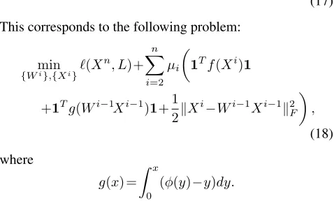
+µi+1(Wi)T(φ(WiXi)−Xi+1), i= 2,· · · , n−1. (17) This corresponds to the following problem:
min
{Wi},{Xi}`(X n, L)+
n
X
i=2 µi
1Tf(Xi)1
+1Tg(Wi−1Xi−1)1+1 2kX
i−Wi−1Xi−1k2
F
,
(18) where
g(x) = Z x
0
(φ(y)−y)dy.
g(X)is also defined element-wise for a matrixX. Thef(x)’s andg(x)’s of some representative activation functions are shown in Table 1. (18) is the formulation of our proposed LPOM, where we highlight that the introduction ofgis non-trivial and non-obvious.
Advantages of LPOM
Denote the objective function of LPOM in (18) asF(W, X). Then we have the following theorem:
Theorem 1 Suppose`(Xn, L)is convex inXnandφis non-decreasing. ThenF(W, X)is block multi-convex, i.e., convex in eachXiandWiif all other blocks of variables are fixed.
Proof.F(W, X)can be simplified to F(W, X) =`(Xn, L)+
n
X
i=2 µi
1Tf˜(Xi)1
+1Tg(W˜ i−1Xi−1)1−hXi, Wi−1Xi−1i, (19)
wheref˜(x) =Rx 0 φ
−1(y)dyandg(x) =˜ Rx
0 φ(y)dy. Since both φ and φ−1 are non-decreasing, both f˜(x) and ˜g(x) are convex. It is easy to verify that1Tg(W˜ i−1Xi−1)1is convex inXi−1whenWi−1is fixed and convex inWi−1 whenXi−1is fixed. The remaining termhXi, Wi−1Xi−1i inF(W, X)is linear in one block when the other two blocks are fixed. The proof is completed. Theorem 1 allows for efficient BCD algorithms to solve LPOM and guarantees that the optimal solutions for updating Xi andWi can be obtained, due to the convexity of sub-problems. In contrast, the subproblems in the penalty and the ADMM based methods are all nonconvex.
When compared with ADMM based methods (Taylor et al. 2016; Zhang, Chen, and Saligrama 2016), LPOM does not re-quire Lagrange multipliers and more auxiliary variables than
{Xi}n
i=2. Moreover, we have designed delicate algorithms so that no auxiliary variables are needed either when solving LPOM (see Section “Solving LPOM”). So LPOM has much less variables than ADMM based methods and hence saves memory greatly. Actually, its memory cost is close to that of SGD as SGD needs to save{Xi}n
i=2.
When compared with the penalty methods (Carreira-Perpinan and Wang 2014; Zeng et al. 2018), the optimality conditions of LPOM are simpler. For example, the optimality conditions for {Xi}n−1
i=2 and{W
i}n−1
i=1 in LPOM are (17) and
(φ(WiXi)−Xi+1)(Xi)T=0, i= 1,· · ·, n−1, (20) while those for MAC are
(Xi−φ(Wi−1Xi−1))
+ (Wi)T[(φ(WiXi)−Xi+1)◦φ0(WiXi)] =0, i= 2,· · · , n−1.
(21)
and
where◦denotes the element-wise multiplication. We can see that the optimality conditions for MAC have extraφ0(WiXi), which is nonlinear. The optimality conditions for (Zeng et al. 2018) can be found in Supplementary Materials. They also have an extraφ0(Ui). This may imply that the solution sets of MAC and (Zeng et al. 2018) are more complex and also “larger” than that of LPOM. So it may be easier to find good
solutions of LPOM.
When compared with the convex optimization reformula-tion methods (Zhang and Brand 2017; Askari et al. 2018), LPOM can handle much more general activation functions. Note that Zhang and Brand (2017) only considered ReLU. Although Askari et al. (2018) claimed that their formulation can handle general activation functions, its solution method was still restricted to ReLU. Moreover, Askari et al. (2018) do not have a correct reformulation as its optimality conditions for{Xi}n−1
i=2 and{Wi}
n−1
i=1 are
0∈µi(φ−1(Xi)−Wi−1Xi−1)−µi+1(Wi)TXi+1, i= 2,· · · , n−1,
and
Xi+1(Xi)T=0, i= 1,· · · , n−1,
respectively. It is clear that the equality constraints (14) do not satisfy the above. Moreover, somehow Askari et al. (2018) further added extra constraintsXi≥0, no matter what the activation function is. So their reformulation cannot approxi-mate the original DNN (2) well. This may explain why Askari et al. (2018) could not obtain good results. Actually, they can only provide good initialization for SGD.
When compared with gradient based methods, such as SGD, LPOM can work with any non-decreasing Lipschitz continuous activation function without numerical difficul-ties, including being saturating (e.g., sigmoid and tanh) and non-differentiable (e.g., ReLU and leaky ReLU) and could update the layer-wise weights and activations in parallel in an asynchronous way (see next section)2. In contrast,
gra-dient based methods can only work with limited activation functions, such as ReLU, leaky ReLU, and softplus, in order to avoid the gradient vanishing or blow-up issues, and they cannot be parallelized when computing the gradient and the activations. Moreover, gradient based methods require much parameter tuning, which is difficult (Le et al. 2011), while the tuning of penaltiesµi’s in LPOM is much simpler.
Solving LPOM
Thanks to the block multi-convexity (Theorem 1), LPOM can be solved by BCD. Namely, we updateXiorWiby fixing all other blocks of variables. The optimization can be performed using a mini-batch of training samples, as summarized in Algorithm 1. Below we give more details.
Updating
{
X
i}
n i=2We first introduce the serial method for updating{Xi}n i=2. We update{Xi}n
i=2fromi= 2tonsuccessively, just like the feed-forward process of DNNs. Fori = 2,· · ·, n−1,
2
But our current implementation is still serial.
Algorithm 1Solving LPOM
Input:training dataset, batch sizem1, iteration no.sSand K1.
fors= 1toSdo
Randomly choosem1training samplesX1andL. Solve{Xi}n−1
i=2 by iterating Eq. (25) forK1times (or until convergence).
SolveXnby iterating Eq. (28) forK1times. Solve{Wi}n−1
i=1 by applying Algorithm 2 to (30).
end for
Output:{Wi}n−1
i=1.
with{Wi}n−1
i=1 and other{Xj}nj=2,j6=ifixed, problem (18) reduces to
min
Xi µi
1Tf(Xi)1+1 2kX
i−Wi−1Xi−1k2
F
+µi+1
1Tg(WiXi)1+1 2kX
i+1−WiXik2
F
.
(23)
The optimality condition is:
0∈µi(φ−1(Xi)−Wi−1Xi−1)
+µi+1((Wi)T(φ(WiXi)−Xi+1)).
(24) Based on fixed-point iteration (Kreyszig 1978) and in order to avoid usingφ−1, we may updateXiby iterating
Xi,t+1=φ
Wi−1Xi−1−µi+1 µi
(Wi)T(φ(WiXi,t)−Xi+1)
(25) until convergence, where the superscriptt is the iteration number. The convergence analysis is as follows3:
Theorem 2 Suppose that φ is differentiable and
|φ0(x)| ≤ γ. If ρ < 1, then the iteration is
con-vergent and the convergent rate is linear, where
ρ=µi+1
µi γ 2p
k|(Wi)T||Wi|k
1k|(Wi)T||Wi|k∞.
In the above,|A|is a matrix whose entries are the absolute values ofA,k · k1andk · k∞are the matrix 1-norm (largest
absolute column sum) and the matrix∞-norm (largest abso-lute row sum), respectively. Note that the choice ofρin the above theorem is quite conservative. So in our experiments, we do not obey the choice as long as the iteration converges.
When consideringXn, problem (18) reduces to
min Xn`(X
n, L)+µ n
1Tf(Xn)1+1 2kX
n−Wn−1Xn−1k2
F
. (26) Assume that the loss function is differentiable w.r.t.Xn. The optimality condition is:
0∈ ∂`(X
n, L)
∂Xn +µn(φ
−1(Xn)−Wn−1Xn−1). (27) Also by fixed-point iteration, we may updateXnby iterating
Xn,t+1=φ
Wn−1Xn−1− 1 µn
∂`(Xn,t, L) ∂Xn
(28) until convergence. The convergence analysis is as follows:
3
Theorem 3 Suppose that φ(x) is differentiable and
|φ0(x)| ≤γand
∂2`(X,L)
∂Xkl∂Xpq
1≤η. Ifτ <1, then the
iter-ation is convergent and the convergent rate is linear, where
τ=µγη n.
If`(Xn, L)is the least-square error, i.e.,`(Xn, L) =12kXn− Lk2
F, then
∂2`(X,L)
∂Xkl∂Xpq
1= 1. So we obtainµn> γ.
The above serial update procedure can be easily changed to asynchronously parallel update: eachXiis updated using the latest information of otherXj’s,j 6=i.4
Updating
{
W
i}
ni=1−1{Wi}n−1
i=1 can be updated with full parallelization. When
{Xi}n
i=2are fixed, problem (18) reduces to min
Wi 1
Tg(WiXi)1+1
2kW
iXi−Xi+1k2
F, i= 1,· · · , n−1, (29) which can be solved in parallel. (29) can be rewritten as
min
Wi 1 T
˜
g(WiXi)1−hXi+1, WiXii, (30) whereg(x) =˜ Rx
0 φ(y)dy, as introduced before. Suppose that φ(x)isβ-Lipschitz continuous, which is true for almost all activation functions in use. Theng(x)˜ isβ-smooth:
|˜g0(x)−g˜0(y)|=|φ(x)−φ(y)| ≤β|x−y|. (31) Problem (30) could be solved by APG (Beck and Teboulle 2009) by locally linearizingˆg(W) = ˜g(W X). However, the Lipschitz constant of the gradient ofˆg(W), which isβkXk2
2, can be very large, hence the convergence can be slow. Below we propose a variant of APG that is tailored for solving (30) much more efficiently.
Consider the following problem: min
x F(x)≡ϕ(Ax) +h(x), (32)
where bothϕ(y)andh(x)are convex. Moreover,ϕ(y)isLϕ -smooth:k∇ϕ(x)−∇ϕ(y)k ≤Lϕkx−yk,∀x, y.We assume that the following problem
xk+1= argmin
x
h∇ϕ(Ayk), A(x−yk)i+ Lϕ
2 kA(x−yk)k
2+h(x) (33) is easy to solve for any givenyk. We propose Algorithm 2 to solve (32), which naturally comes from the proof of its convergence theorem:
Theorem 4 If we use Algorithm 2 to solve problem (32), then the convergence rate is at leastO(k−2):
F(xk)−F(x∗)+ Lϕ
2 kzkk
2≤ 4
k2
F(x1)−F(x∗)+
Lϕ 2 kz1k
2
,
wherezk=A[θk−1xk−1−xk+(1−θk−1)x∗]andx∗is any
optimal solution to problem(32).
4
The convergence can be proven when the objective function is augmented with a proximal term σ
2kX
i−
Xi,0k2
F, whereXi,0is
chosen as the last update ofXi. As the implementation and analysis of asynchronously parallel update deserve an independent paper, we choose not to squeeze them in this paper.
Algorithm 2Solving (32).
Input:x0,x1,θ0= 0,k= 1, iteration no.K2.
fork= 1toK2do Computeθkvia1−θk=
√
θk(1−θk−1). Computeykviayk=θkxk−
√
θk(θk−1xk−1−xk). Updatexk+1via (33).
end for Output:xk.
Problem (30) is an instantiation of (32). Accordingly, the instantiation of subproblem (33) is as follows:
Wi,t+1= argmin
W
φ(Yi,tXi),(W−Yi,t)Xi
+β
2k(W−Y
i,t)Xik2
F−hX
i+1, W Xii. (34)
It is a least-square problem and the solution is: Wi,t+1=Yi,t−1
β(φ(Y
i,tXi)−Xi+1)(Xi)†, (35)
where(Xi)†is the pseudo-inverse ofXiandYi,tplays the role ofykin Algorithm 2.
Experiments
We evaluate LPOM by comparing with SGD and two non-gradient based methods (Askari et al. 2018; Taylor et al. 2016). The other non-gradient based methods do not train fully connected feed-forward neural networks for classifica-tion tasks (e.g., using skip connecclassifica-tions (Zhang and Brand 2017), training autoencoders (Carreira-Perpinan and Wang 2014), and learning for hashing (Zhang, Chen, and Saligrama 2016)). So we cannot include them for comparison. For sim-plicity, we utilize the least-square loss function and the ReLU activation function unless specified otherwise. Unlike (Askari et al. 2018), we do not use any regularization on the weights
{Wi}n−1
i=1. We run LPOM and SGD with the same inputs and random initializations (Glorot and Bengio 2010). We imple-ment LPOM with MATLAB without optimizing the code. We use the SGD based solver in Caffe (Jia et al. 2014). For the Caffe solver, we modify the demo code and carefully tune the parameters to achieve the best performances. For (Askari et al. 2018), we quote their results. For (Taylor et al. 2016), we read the results from Fig.1 (b) of the paper.
Comparison with SGD
We conduct experiments on two datasets, i.e., MNIST5and
CIFAR-10 (Krizhevsky and Hinton 2009). For the MNIST dataset, we use28×28 = 784raw pixels as the inputs. It in-cludes 60,000 training images and 10,000 test images. We do not use pre-processing or data augmentation. For LPOM and SGD, in each epoch the entire training samples are passed through once. The performance depends the choice of net-work architecture. Following (Zeng et al. 2018), we imple-ment a 784-2048-2048-2048-10 feed-forward neural network.
5
0 20 40 60 80 100 Epochs
0.85 0.9 0.95 1
Training accuracy
LPOM SGD
0 20 40 60 80 100 Epochs
0.88 0.9 0.92 0.94 0.96 0.98 1
Test accuracy
LPOM SGD
(a) MNIST (Training Acc.) 0 20 40 60 80 100
Epochs 0.85
0.9 0.95 1
Training accuracy
LPOM SGD
0 20 40 60 80 100 Epochs
0.88 0.9 0.92 0.94 0.96 0.98 1
Test accuracy
LPOM SGD
(b) MNIST (Test Acc.)
0 20 40 60 80 100 Epochs
0.2 0.4 0.6 0.8 1
Training accuracy
LPOM SGD
0 20 40 60 80 100 Epochs
0.35 0.4 0.45 0.5 0.55
Test accuracy
LPOM SGD
(c) CIFAR-10 (Training Acc.) 0 20 40 60 80 100
Epochs 0.2
0.4 0.6 0.8 1
Training accuracy
LPOM SGD
0 20 40 60 80 100 Epochs
0.35 0.4 0.45 0.5 0.55
Test accuracy
LPOM SGD
(d) CIFAR-10 (Test Acc.)
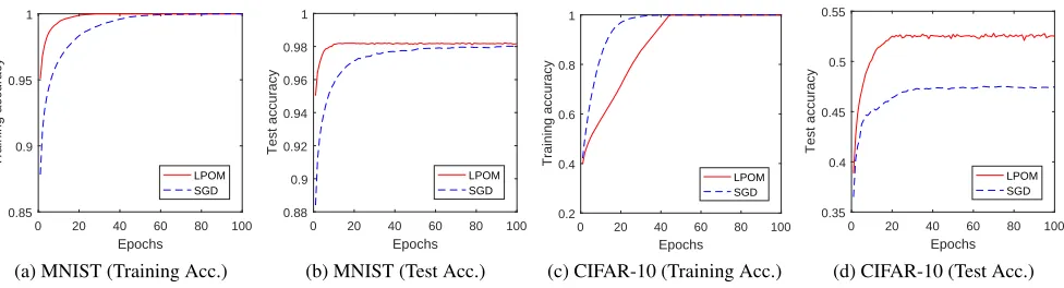
Figure 1: Comparison of LPOM and SGD on the MNIST and the CIFAR-10 datasets.
Table 2: Comparison of accuracies of LPOM and (Askari et al. 2018) on the MNIST dataset using different networks. Hidden layers 300 300-100 500-150 500-200-100 400-200-100-50
(Askari et al. 2018) 89.8% 87.5% 86.5% 85.3% 77.0%
LPOM 97.7% 96.9% 97.1% 96.2% 96.1%
Table 3: Comparison with SGD and (Taylor et al. 2016) on the SVHD dataset.
SGD 95.0%
(Taylor et al. 2016) 96.5%
LPOM 98.3%
For LPOM, we simply setµi= 20in (18). We run LPOM and SGD for 100 epochs with a fixed batch size 100. The training and test accuracies are shown in Fig. 1 (a) and (b). We can see that the training accuracies of the two methods are both approximately equal to100%. However, the test accuracy of LPOM is slightly better than that of SGD (98.2%vs.98.0%).
For the CIFAR-10 dataset, as in (Zeng et al. 2018) we implement a 3072-4000-1000-4000-10 feed-forward neural network. We normalize color images by subtracting the train-ing dataset’s means of the red, green, and blue channels, respectively. We do not use pre-processing or data augmen-tation. For LPOM, we setµi= 100in (18). We run LPOM and SGD for 100 epochs with a fixed batch size 100. The training and test accuracies are shown in Fig. 1 (c) and (d). We can see that the training accuracies of SGD and LPOM are approximately equal to100%. However, the test accuracy of LPOM is better than that of SGD (52.5%vs.47.5%).
Comparison with Other Non-gradient Based
Methods
We compare against (Askari et al. 2018) with identical ar-chitectures on the MNIST dataset. Askari et al. (2018) only use the ReLU activation function in real computation. As in (Askari et al. 2018), we run LPOM for 17 epochs with a fixed batch size 100. For LPOM, we setµi= 20for all the networks. We do not use pre-processing or data augmentation. The test accuracies of the two methods are shown in Table 2. We can see that LPOM with the ReLU activation function performs better than (Askari et al. 2018) with significant gaps.
This complies with our analysis in Subsection “Advantages of LPOM”.
Following the settings of dataset and network architecture in (Taylor et al. 2016), we test LPOM on the Street View House Numbers (SVHN) dataset (Netzer et al. 2011). For LPOM, we setµi= 20in (18). The test accuracies of SGD, (Taylor et al. 2016), and LPOM are shown in Table 3. We can see that LPOM outperforms SGD and (Taylor et al. 2016). This further verifies the advantage of LPOM.
Conclusions
In this work we have proposed LPOM to train fully connected feed-forward neural networks. Using the proximal operator, LPOM transforms the neural network into a new block multi-convex model. The transformation works for general non-decreasing Lipschitz continuous activation functions. We apply the block coordinate descent algorithm to solve LPOM, where each subproblem has convergence guarantee. LPOM does not require more auxiliary variables than the layer-wise activations and its penalties are relatively easy to tune. It could also be solved in parallel in an asynchronous way. Our experimental results show that LPOM works better than SGD, (Askari et al. 2018), and (Taylor et al. 2016) on fully connected neural networks. Future work includes extending LPOM to train convolutional and recurrent neural networks and applying LPOM to network quantization.
Acknowledgements
Z. Lin is supported by 973 Program of China (grant no. 2015CB352502), NSF of China (grant nos. 61625301 and 61731018), Qualcomm, and Microsoft Research Asia.
References
Beck, A., and Teboulle, M. 2009. A fast iterative shrinkage-thresholding algorithm for linear inverse problems. SIAM Journal on Imaging Sciences183–202.
Carreira-Perpinan, M., and Wang, W. 2014. Distributed optimization of deeply nested systems. InInternational Con-ference on Artificial Intelligence and Statistics, 10–19. Collobert, R.; Weston, J.; Bottou, L.; Karlen, M.; Kavukcuoglu, K.; and Kuksa, P. 2011. Natural language processing (almost) from scratch. Journal of Machine Learn-ing Research12:2493–2537.
Dauphin, Y.; de Vries, H.; and Bengio, Y. 2015. Equili-brated adaptive learning rates for non-convex optimization. In Advances in Neural Information Processing Systems, 1504–1512.
Duchi, J.; Hazan, E.; and Singer, Y. 2011. Adaptive subgradi-ent methods for online learning and stochastic optimization.
Journal of Machine Learning Research12:2121–2159. Ge, R.; Huang, F.; Jin, C.; and Yuan, Y. 2015. Escaping from saddle points-online stochastic gradient for tensor decompo-sition. InConference on Learning Theory, 797–842. Glorot, X., and Bengio, Y. 2010. Understanding the difficulty of training deep feedforward neural networks. In Proceed-ings of the Thirteenth International Conference on Artificial Intelligence and Statistics, 249–256.
He, K.; Zhang, X.; Ren, S.; and Sun, J. 2016. Deep residual learning for image recognition. InProceedings of the IEEE Conference on Computer Vision and Pattern Recognition, 770–778.
Hinton, G.; Deng, L.; Yu, D.; Dahl, G. E.; Mohamed, A.-R.; Jaitly, N.; Senior, A.; Vanhoucke, V.; Nguyen, P.; Sainath, T. N.; et al. 2012. Deep neural networks for acoustic model-ing in speech recognition: The shared views of four research groups. IEEE Signal Processing Magazine29(6):82–97. Hubara, I.; Courbariaux, M.; Soudry, D.; El-Yaniv, R.; and Bengio, Y. 2016. Binarized neural networks. InAdvances in Neural Information Processing Systems, 4107–4115. Jia, Y.; Shelhamer, E.; Donahue, J.; Karayev, S.; Long, J.; Girshick, R.; Guadarrama, S.; and Darrell, T. 2014. Caffe: Convolutional architecture for fast feature embedding. In
Proceedings of the 22nd ACM International Conference on Multimedia, 675–678. ACM.
Kingma, D. P., and Ba, J. 2014. Adam: A method for stochas-tic optimization.arXiv preprint arXiv:1412.6980.
Kreyszig, E. 1978. Introductory Functional Analysis with Applications, volume 1. Wiley New York.
Krizhevsky, A., and Hinton, G. 2009. Learning multiple lay-ers of features from tiny images. Technical report, Univlay-ersity of Toronto.
Krizhevsky, A.; Sutskever, I.; and Hinton, G. E. 2012. Ima-genet classification with deep convolutional neural networks. In Advances in Neural Information Processing Systems, 1097–1105.
Le, Q. V.; Ngiam, J.; Coates, A.; Lahiri, A.; Prochnow, B.; and Ng, A. Y. 2011. On optimization methods for deep learning. InProceedings of the 28th International Conference
on International Conference on Machine Learning, 265–272. Omnipress.
Lin, Z.; Liu, R.; and Su, Z. 2011. Linearized alternating direction method with adaptive penalty for low-rank repre-sentation. InAdvances in Neural Information Processing Systems, 612–620.
Netzer, Y.; Wang, T.; Coates, A.; Bissacco, A.; Wu, B.; and Ng, A. Y. 2011. Reading digits in natural images with unsupervised feature learning. InNIPS workshop on Deep Learning and Unsupervised Feature Learning, volume 2011, 5.
Parikh, N., and Boyd, S. 2014. Proximal algorithms. Foun-dations and TrendsR in Optimization1(3):127–239. Rumelhart, D. E.; Hinton, G. E.; and Williams, R. J. 1986. Learning representations by back-propagating errors. Nature
323(6088):533.
Silver, D.; Huang, A.; Maddison, C. J.; Guez, A.; Sifre, L.; Van Den Driessche, G.; Schrittwieser, J.; Antonoglou, I.; Panneershelvam, V.; Lanctot, M.; et al. 2016. Mastering the game of Go with deep neural networks and tree search.
Nature529(7587):484.
Sutskever, I.; Martens, J.; Dahl, G.; and Hinton, G. 2013. On the importance of initialization and momentum in deep learning. InInternational Conference on Machine Learning, 1139–1147.
Taylor, G.; Burmeister, R.; Xu, Z.; Singh, B.; Patel, A.; and Goldstein, T. 2016. Training neural networks without gradi-ents: A scalable ADMM approach. InInternational Confer-ence on Machine Learning, 2722–2731.
Zeng, J.; Ouyang, S.; Lau, T. T.-K.; Lin, S.; and Yao, Y. 2018. Global convergence in deep learning with variable splitting via the Kurdyka-łojasiewicz property.arXiv preprint arXiv:1803.00225.
Zhang, Z., and Brand, M. 2017. Convergent block coordi-nate descent for training Tikhonov regularized deep neural networks. InAdvances in Neural Information Processing Systems, 1721–1730.