“Numerical Solution of Irrotational Fluid Flow
Problem Using Finite Element Method”
Rajesh Kumar Pal
Ast. Professor, DAV(PG) College, Dehradun (U.K.) India- 248001
Abstract
The Finite Element Method has its advancement over other finite difference methods due to taken into consideration the irregular shape domain of problem. The domain of interest on which problem is defined has to be subdivided into sub domains. Herein, two irregular-shaped domain are considered and elliptic equations are solved in each domain with the boundary conditions having varies nature i.e. Dirichlet, Neumann and mixed conditions are applied. Detail discretisation of Finite Element Method and Weighted Residual Techniques are also discussed with their prerequisite conditions. So this Method is a novel fast elliptic solver that can serves as a feasible alternative for numerical solutions and the results compare well with those of [18].
Keywords: Poisson’s equation, Weighted Residual Techniques, Finite Element Methods, Galerkin method.
I. INTRODUCTION
A variety of physical phenomenon is governed by elliptic equation viz. Laplace-equation, Poisson-equation and Navier- Stokes Poisson-equation. Following Poisson-equation
with suitable boundary conditions constitutes an elliptic boundary value problem. Consider a boundary value problem given by
L u=f in domain D ……… (2)
which is bounded by S with appropriate boundary conditions prescribed on S , where L is differential operator and f is a known function. Weighted residual techniques are a pre-requisite for Finite Element Methods. The underlying principle of weighted residual method is that instead of looking for solution which satisfies (2) exactly at every point of D, we go for an approximate solution u that satisfies it in a weaker form. Let us represent approximate solution that satisfies boundary condition as
Where u‟s are parameters to be determined. We substitute (3) in (2) and obtain resulting function known as residual denoted by R so that
R= L u –f ………..(4)
In a Weighted residual method, the integral of residual R along with certain weights is minimised over domain D . In Galerkin method, we assume that basis functions i, i=1(1)n are orthogonal to R over D i.e.
The n equations given by (5) provide values of unknowns. ai,s which upon substitution in (2) give approximate solution.
Before applying Finite Element Methods, the domain of interest on which problem is defined has to be subdivided into sub domains. These subdomains are known as „elements‟. The elements may be of any shapes or sizes. We prefer to triangular and rectangular shapes only due to simplicity in computations and due to their wide applicability.
It is arbitrary subdivision of the domain which places the Finite Elements Methods much above the finite difference methods. Because of this flexibility, very fine elements may be chosen near the sensitive points of D and larger elements may be chosen where behavior of the solution is expected to be quite smooth.
) 3 ..( ... ...
1
n
i
i i
u
u
D D
i
ids Lu f ds i n
R 0, 1(1) ... .(5)
, , , ... ..(1) 2
2
2 2
o y x c y u y x b x u y x a y
u x
u
II.DIFFERENTAPPROACHESTRIEDFORTHEPROBLEM
In the earliest investigations, elliptic boundary value problem was solved by applying finite difference techniques (See Burggraf [5], Mills [15]). Solution techniques for Laplace‟s and Poisson‟s equation have been developed by Hockney [10] and Sharma and Agarwal [16] . Liniger et al [13] have applied method of pre-conditioner for solution of Poisson‟s equation. Multigrid methods ( Macormic [14] and Bramble et al [4] ) have also been employed for this equation. Liniger et al [13] and Hyman and Manteuffel [11] have applied high-order sparse factorization methods for elliptic boundary value problems. Bennour and Said [2] have also applied Numerical method with Dirichlet boundary conditions. But as Chang [7] states himself that Finite Difference Solution algorithms are not directly applicable to an elliptic problem with a computational domain of irregular shape.
Finite Element Methods had their origin in the problem related to „Solid Mechanics‟ (see, Zienkiewicz, [19]). The success of these techniques in solid mechanics in late 1960‟s and early 1970‟s gave an impetus for utilisation of this method in „Fluid Mechanics‟. It was thought that significant advantages gained in structural mechanics would also be helpful in Fluid Mechanics . The range of problems encountered in fluid mechanics is so great that there was need for a technique flexible in its approach and having versatility. Due to its great flexibility, Finite Element Methods using linear trial and test function for Poisson‟s was applied by Tuann and Olson [18]. Barrett and Demunshi [1] have taken up exponential test and trial function. Finite element methods for fluid flow problems of various nature are discussed by Bercovier and Engelman [3] , Girault and Raviart [9]. In the past several years, novel Numerical approaches have been applied by Cai et. al. [6] , Chaudhary and Patel [8] using different boundary conditions.
III.FINITEELEMENTMETHODSFORPOISSON’S EQUATION
Consider the Poisson‟s equation in two dimensions as
in D where D is enclosed by a curve S. Solution is to be obtained in the region DUS.
Let S = S1U S2US3US4 with Dirichlet‟s boundary conditions on S1 and S3 and Neumann boundary conditions on S2 and S4 . We subdivide the domain D into M elements giving rise to N nodes whose coordinates are known.
Let the approximate solution of (6) in D, be expressed as
Where I‟s are the global shape functions such that i =1 at node i and zero at all the other nodes i.e. if (xr, yr) denotes the rth node then i (xr, yr) = ir . We adopt Galerkin‟s criterion to find u‟s in (3). And the residual is given by,
Following Galerkin‟s criterion the resulting equations would be,
After substituting R(x,y) from (7), the equation (8) becomes,
, 0... ... ....( 6) 2 2 2 2 y x q y u x u ) 7 ....( ... 0 ) , ( ) , ( 2 2 2 2
q x y
y u x u y x R N i dxdy y x R D i ) 1 ( 1 ) 8 . . . ( . . . . 0 ) , (
) 9 .( ... 0 ) , ( 2 2 2 2
q x y dxdyAfter applying vector vector calculus formulae, above equation reduces to,
The integral appearing in (10) is evaluated element by element. Thus (10) may be written as
i =1(1)N
Where er denotes the rth element and the line integral is taken over the sides of the boundary elements which form S. We will put (11) in matrix form. Thus it may be written as ,
Pu =R+T ……….(12)
where uT =(u1 , u2 ,u3 …………., uN); the coefficient matrix P is (NXN) matrix, R and T are column matrices each of order N. Evaluation of P,R and T in (12) is performed elementwise. They are,
Where Sp denotes the side (s) of boundary element which approximate s, ds denotes the elemental length along
the side approximating the boundary.
IV.EVALUATIONOFVARIOUSTERMSFOR ER:-
Let us assume that the rth element er is performed by joining the three nodes l, m and n whose coordinates are (x1, y1), (xm ym) and (xn, yn) respectively. The various terms in the element are evaluted as follows:-
A. Evaluation of Pr
The matrix Pr , in terms of local coordinates , will have the following form,
Pr = Ar
a12+ b12 a1 a2 +b1b2 a1a3 +b1b3 a1 a2 +b1b2 a12+ b12 a2a3 +b2b3 a1a3 +b1b3 a2a3 +b2b3 a32+ b32
……(16)
Where values of a1, b1 c1 etc. are obtained as, a1 = 1/2Ar(y2 -y3)
b1 = - 1/2Ar(x2 -x3)
and c1 = 1/2 Ar (x2y3 –y2x3 ) etc. …..…….(17)
Ar being the area of the element er .
B. Evaluation of Rr
From equation (14) we have,
Again for I=1,m or n , Rr(i)=0. Let us assume that the value of q(x,y) remains constant over the er , so that we can take qr(x,y)=qr (constant). Therefore, (18) may be written as
C. Evaluation of Tp
Let ep be boundary element whose nodes l,m and n are identified with the coordinates (xl, yl), (xm ym) and (xn, yn). Let us assume that only one side , say slm
forms part of SD (figure 6.1) then the line integral on this side is given by
n
L m
Ql
Qm
Fig. 1 Nodes of the Boundary Elements
N i
dxdy q
i R
r e
i r
) 1 ( 1
) 18 .( ... )
(
n m l i
dxdy q
i R
r
e i r r
, ,
) 19 ( )
(
N i
ds Q
i
T i
S p
l m
) 1 ( 1
) 20 ...(
... ,...
) (
Here, since i is zero on ep for I l,m,n , the value of Tp(i) will be zero for every i except i =l,,m and n . Now since x remains zero all along the side Slm ,
Also we have,
Thus there remain only two terms to be evaluated, namely Tp(l) and Tp(m). Referring to nodes l, m and n as 1,2 and 3 as their local counterparts respectively, we shall have from (20),
Tp(3) =0 ………..(22) And from (21) we have,
D. Assembly of Various Elements
Having computed Pr and Rr for each element er , r=1(1)M and Tp for each boundary element, we wish to put the respective entries at appropriate positions in P,R and T in equation (6.12). Since all the computations have been made in terms of local nodes we wish to have an elementwise reference table connecting the local names with their global names. Such a table is known as connectivity table which will have following format for the rth element er whose global nodes l,m,n are taken to be 1,2,3 respactively. The order of l,m,n is immaterial.
Table 1- Connectivity table
Element Number Node 1 Node 2 Node 3
R l M n
E. Solution of Equations
After the final assembly we arrive at as many equations as there are nodes i.e. N. Depending on the boundary conditions, some of the values of u may be known. Transferring these terms to RHS, we solve the remaining system by Gauss-Jordan‟s direct method.
V. PROBLEM-I
Consider a steady- state equation 2
u + 3(2x-y) = 0 in D ………(24)
) 21 ...( ...
) ( ,
) (
1 1
1ds and T m Q ds
Q l
T m
S p
S p
m m
)
23
...(
...
)
2
(
;
)
1
(
2 1
12 12
ds
Q
T
and
ds
Q
T
S p
S p
lm
S x p x Q ds
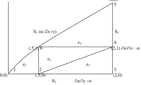
where D is bounded by S= S1 U S1 U S3. The curves with approximate boundary conditions on them are defined as,
(i) S1 : y2 = 2x where u= 2x+y ( Dirichlet Condition) ……….(25) (ii) S2 : y=0 where u/y =o, (Neumann Condition)……….(26) (iii) S3 : x=0 where u/x = -u (Mixed Condition) ……..…(27)
We solve the problem defined by (24) –(27) by Finite Element Methods subdividing the domain into four triangular elements in the manner as shown in figure 2.
(2,2) 5
S1 (u=2x+y) S3
e4 4
(.5,1) 6 (2,1) u/x= -u
e2
e1 e3
1 2 3 (0,0) (.5,0) (2,0) S2 u/y =o
Fig. 2 Triangular Elements of the Domain
VI.SOLUTION
Here the domain D is subdivided into four elements e1, e2, e3 and e4 with six nodes , say NI , i=1(1)6. First of all we have to fix the coordinates of the nodes. We see that the values of u1, u6 and u5 are known; they are u1=0, u6=2 and u5=6. Therefore only u2, u3 and u4 have to be calculated .
Next we draw a connectivity table for associating the global nodes with the local ones.
Table 2. Connectivity Table
Element Number Node 1 Node 2 Node 3
1 2 3 4
1 2 2 4
2 4 3 5
6 6 4 6
We calculate the areas of the various elements which are given below as: Area of e1 =.25
Area of e2 =.75 Area of e3 =.75 Area of e4 =.75
Comparing the given problem with (6.6), here q(x,y)= 3(2x-y). Now various terms of Pr, Rr and Tp can be computed elementwise.
A. Element e1
Therefore P1 in matrix form is,
P1 =
1.0 -1.0 0
-1.0 1.25 -0.25 0 -0.25 0.25 ………..(28)
R1 can be calculated by taking the value of q(x,y) to be constant over an element, we may choose its value at x= (x1 +x2 +x3)/3, y = (y1 +y2 +y3 )/3 in each element. So .0833
R1 = .0833
.0833
……….(29)
We see that S12 and S31 approximate part of the boundary S of the domain D. Therefore, we shell have, T1 (i) = T11 (i) + T12 (i) , i=1,2,3 ……….(30)
where So we get T1 = T11 +T12 = 2 Q1 +Q3 0
Q1 + 2Q3 ………….(31)
where Q1and Q3 in (31) are not known. B. Element e2 Here the global nodes 2,4 and 6 are locally taken to be 1,2 and 3 respectively. The coordinates are given as (x1,y1)=(0.5,0); (x2,y2)=(2,1); (x3,y3)=(.5,1). Here we have P2 = 0.75 0.0 -.75
0.0 1/3 - 1/3 -.75 - 1/3 13/12 ………..(32)
1.0 R2 = 1.0 1.0 ………(33)
Since element e2 is not a boundary element i.e. none of its sides form part of the boundary, it will play no part in the line integral.
C. Element e3
The global elements 2, 3 and 4 in this element are taken to be 1,2 and 3 receptively as their local counterparts. Their coordinates are,
. )
( ,
) (
31 12
12
11 i Q ds and T i Q ds
T i
S i
S
(x1,y1)=(0.5,0); (x2,y2)=(2,0); (x3,y3)=(2,1).
Therefore P3 is-
P3 =
1/3 -1/3 0 -1/3 1/3 0 0 0 3/4
……….(34) And
2.0 R3 = 2.0 2.0
………..(35) We have from (20)
T3= T31 (i)+T33(i) , say
0
T3 = 1/3u2+1/6u3 1/6u2+1/3u3
…….(36)
D. Element e4
Referring to the connectivity table we note that the local nodes 1, 2 and 3 are taken to be as N4 ,N5 and N6 respectively. Let us write down coordinates of these nodes in local terms,
(x1,y1)=(2,1); (x2,y2)=(2,2); (x3,y3)=(.5,1).
So P4 is-
P4 =
13/12 -3/4 -1/3 -3/4 3/4 0 -1/3 0 1/3
……….(37) And
5/4 R4 = 5/4
5/4
………..(38) We have ,
T4 (i) = T41 (i)+T42(i) , say
T4 =
1/3u1+1/6 u2+0 1/6u1+1/3u2+.6Q2+.3Q3 0+.3Q2+.6Q3
…….(39)
VII. ASSEMBLEYOFELEMENTS
As soon as Pr ,Rr and Tr are computed for an element, their components are placed at the appropriate positions in the final matrices P , R and T to form equation (6.12). As explained earlier P is a (6x6) matrix and R and T are (6X1) each.
This is a system of algebraic equation and can be solved by any standard technique. We have applied Gauss- Jordan‟s method and values of unknowns are obtained as :
u2 =0.865, u3 =2.809 u4 =2.604.
3 , 2 , 1 ,... )
(
23 12
3 i
Q ds
Q ds i T i
S i S
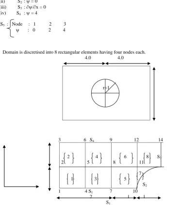
VIII. PROBLEM II :-
Stream function for a two-dimensional flow of incompressible irrotational flow around a cylinder is given by
2 =0
Domain D is bonded by S=S1U S2U S3 U S3U S4U S5 with boundary conditions defined as- (i) S1 : = 0
(ii) S2 : = 0 (iii) S3 : /x = 0 (iv) S4 : = 4
S5 : Node : 1 2 3 : 0 2 4
Domain is discretised into 8 rectangular elements having four nodes each. 4.0 4.0
3 6 S4 9 12 14
2
2
1 4 5
3
6 8
5
8 S3
11
7
S2 1 4 S1 7 10 2 1 1
S1
Fig. 3 Irrotational flow around a cylinder, Element distribution and boundary conditions
The simplest form of interpolating function for 4-noded rectangular elements is given by- (x,y)=ax+by+c+dxy
as in previous example, we express (x,y) in terms of shape function (x,y) = 11 +22 +33+44
where i‟s are function of x and y having a property that i=1, i=1(1)4 at node i and zero at remaining ones. As for triangular elements, we obtain values of i, i=1(1)4 as
1(,)=(1-)(1-) 2(,)=(1-) 3(,)=. 4(,)=(1-) 0, 1
x1xx2 y1yy2
Remaining calculations are carried out exactly in the same manner as in previous problem. Solving the final system of equations, we obtain the values of inter nodes as
5 1.96 8 = 1.78 11 1.09
IX. CONCLUSION
Two problems governed by elliptic partial differential equations have been considered. We have proposed and developed an efficient Numerical method for solving Poisson problem. It can deal with Poisson‟s equation with Neumann, Dirichlet as well as mixed boundary conditions in a 2-D irregular region. The first problem is taken as a test problem of Poisson‟s equation with the general type of domain and with both types of boundary conditions viz. Dirichlet and Neumann. The Finite Element Methods presented here works well with the problem. The second problem is important from application point of view and was considered by Taylor and Hughes [17]. This problem depicts the flow of irrotational flow around a cylinder. For this problem, rectangular elements with their nodes are considered in place of triangular elements as in problem I. The results compare well with those of [18] and [6]. While they have used isoparametric elements. Domains of both the problems are of such a nature that Finite Difference Methods is not suitable for these. The above illustrations show the versatility of Finite Elements Methods over Finite Difference Methods in case of irregular domains. However appropriate choice between Finite Difference Methods and Finite Element Methods depends on the nature of equation, boundary conditions imposed and shape of domain. According to our Numerical experiments, it is observed that the computational complexity of this method is close to O(N) and increase in the number of grid points give rise to an increase in the accuracy of the FEM solutions as discussed in [8] and [12]. So this method is a novel fast elliptic solver that can serves as a feasible alternative for numerical solutions of Poisson as well as Laplace equation.
REFERENCES
[1] Barrett, K.E. and Diminish, G., Finite Element solutions of convective diffusion problems, Int. J. Num. Meth. Eng., 14, 1511-1524, 1979.
[2] Bennour, H. and Said, M. J., Finite Element solutions of convective diffusion problems, Int. J. Num. Meth. Eng., 14, 1511-1524, 1979. [3] Bercovier, M. and Engelman,M., Numerical Solution of Poisson‟s equation with Dirichlet Boundary conditions, Int. J. open problems
compt. Math.,Vol. 5, No. 4, 2012.
[4] Bramble, J.H., Pasciak, J.E. and Schatz, A.H., „The construction of preconditioners for elliptic problems‟, Mathematics of Computation, Vol. 53, No.187, pp.1-24, 1989.
[5] Burggraf, O.R., Analytical and Numerical studies of the structure of steady separated flows, J.Fluid Mech., 24, 113-151,1966. [6] Cai, Z., Kim, S. and Kong, S., A finite element method using singular function for Poisson equation: mixed boundary conditions,
Comput. Methods Appl. Mech. Engrg., 195, pp 2635-2648, 2006.
[7] Chang , S.C., Solution of Elliptic Partial Differential Equations by fast Poisson solvers using a Local Relaxation Factor. I. One step method‟ NSA technical paper 2529, 1986.
[8] Chaudhary, T.U. and Patel, D.M., Finite Element Solution of Poisson‟s equation in a Homogeneous Medium, International Research Journal of Engineering and Tech. (IRJET), Vol. 02, Issue 09, 2015.
[9] Girault,V. and Raviart, P.A ., Finite element approximation of the Navier-Stokes equations, Lecture notes in Mathematics 749, Springer, Berlin, 1979.
[10] Hockney, R.W., A fast direct solution of Poisson‟s equation using Fourier analysis, J. assoc. Comput. Mach., 12,95-113,1965. [11] Hyman, J.M. and Manteuffel, T.A., High order sparse factorization methods for elliptic boundary value problems in R. Vichneretsky
and R.S.Stepleman. Eds. Advances in computer methods for partial differential equations. V(IMACS, New Brunswick . NS. 1984) 551-555.
[12] Kikuchi, F. and Saito, H., Remarks on a posteriori error estimation for finite element solutions, J. Comput. Appl. Meth., 199(2), pp 329-336, 2007.
[13] Liniger, W, Odeh,F. And Hara, V., A second order sparse factorization method for Poisson‟s equation with mixed boundary conditions, J. Comp. And App. Math., 44,201-218,1992.
[14] Macormic,S.F., „Multigrid methods for variational problems: Further results‟ SIAM J. Numer. Anal., Vol.21 ,1984,PP.255-263. [15] Mills, R.D., On the closed motion of a fluid in a square cavity, J. Roy. Aero. Soc., 69,116-120,1965.
[16] Sharma,P.K. and Agarwal , M.K., Fast finite difference direct solver for Poisson‟s equation, Indian J. Phy. Nat. Sci. Vol.10, Sec. B, 1989.
[17] Taylor, C and Hughes, T.G., Finite Element Programming of N-S equations, Pineridge Press Limited, Swansea, U.K., 1981. [18] Tuann, S.Y. and Olson, M.D., Review of computing methods for recirculating flows, J. Comp. Phys. 29,1-17,1978. [19] Zienkiewicz, O.C., The Finite Element Method, Tata McGraw-Hill, New Delhi.
x x
x x
y y
y y
1
2 1
1
2 1