Printed in The Islamic Republic of Iran, 2012 © Shiraz University
AN EFFICIENT METHOD BASED ON ABC FOR
OPTIMAL MULTILEVEL THRESHOLDING
*S. A. MOHAMMADI
1, R. AKBARI
2**AND S. H. MOHAMMADI
3 1Dept. of Electrical and Computer Engineering, Tabriz University, Tabriz, I. R. of Iran
2
Dept. of Computer Engineering and Information Technology, Shiraz University of Technology, Shiraz, I. R. of Iran Email: [email protected]
3
Center for Spoken Language Understanding, Oregon Health & Science University, Portland, OR, USA
Abstract– Many efficient bi-level thresholding techniques have been proposed in recent years. Usually, the objective functions, which are used by them, are not appropriate for the multilevel thresholding owing to exponential growth of computational complexity. This work presents a new multilevel thresholding algorithm using Artificial Bee Colony algorithm (ABC) with the Otsu’s objective function. Also, a strategy is used to guess suitable thresholds for initializing the proposed method. This initializing phase used the bi-level Otsu method to find the initial thresholds. These guessed thresholds are used to create a food source around each of them for use in the ABC algorithm as initial population. The presented thresholding method is tested on four popular images. The results show that this method has competitive performance compared to other well-known methods such as Gaussian-smoothing, Symmetry-duality, GA-based and PSO-based algorithms.
Keywords– Segmentation, multilevel thresholding, otsu method, ABC algorithm
1. INTRODUCTION
Image segmentation is one of the most fundamental processes for image analysis and explanation. This process is used for distinct objects in an image from its background or distinguishing an object from other objects with different gray-levels. One of the methods used broadly in image segmentation is image thresholding. It can be categorized into two classes which are called bi-level thresholding and multilevel thresholding. Bi-level thresholding partitions pixels into two distinct classes; one of the classes comprises those pixels having gray level values above a predefined threshold and the other class includes the rest of the pixels. Multilevel thresholding splits the pixels into various classes and the pixels within a class have a gray level inside a particular range. In this method, a single gray-level value is assigned to each class. One effective and beneficial tool used for evolution of image segmentation is image gray level histograms. Our purpose is to find thresholds, which are gray level values, to classify pixels. The simplest classification is bi-level thresholding in which one threshold should be found, but the problem becomes more complicated if more thresholds need to be found. Generally, it is not straightforward to guess thresholds in the multimodal histogram of an image for image segmentation. Thus multilevel thresholding is an interesting and challenging area of research in the field of image processing.
Many thresholding techniques have been proposed in the past years [1-3]. These techniques can be classified into two distinct groups: optimal thresholding methods [4-8] and property-based thresholding methods [9-11].
Optimal thresholding methods try to find an optimal threshold that segments classes to achieve appropriated attributes. Conventionally, this process is done with optimizing an objective function. Property-based procedures evaluate some properties of histogram for detecting the thresholds.
Received by the editors April 11, 2012; Accepted June 20, 2012.
In recent years many algorithms have been proposed for optimal thresholding, such as maximizing a posteriori entropy to measure the homogeneity of the threshold classes [4-7], an optimal thresholding method to maximize the separateness measures of the classes based on discriminant analysis, which was proposed by Otsu 8] or a minimum error method to minimize the pixel classification error rate proposed by Kittler and Illingworth [ 5]. Because most of these algorithms were originally developed for bi-level thresholding, they encounter the computational complexity, which is exponential when extended to multilevel thresholding due to the exhaustive and comprehensive search. An iterative method was proposed to overcome this problem in [ 12]. It assumed the multilevel thresholding problem as successive bi-level thresholding problems. Then the threshold values were changed to optimize an objective function. This iterative scheme repeated none of the changed threshold values or the threshold could not move. Unfortunately, this method traps local optima with three or more thresholds.
There are also some proposed methods for property-based thresholding. For instance, a method which first smooths the gray-level histogram by the Gaussian convolution has been developed by Lim and Lee [ 11]. Then the first and second derivatives of the smoothed histogram are used to detect thresholds. Another method which has been proposed by Tsai 10] works with unimodal histograms by including a local maximum curvature method to recognize the thresholds. Property-based thresholding methods are rapid and appropriate for the case of multilevel thresholding, while the number of thresholds is difficult to determine and should be given beforehand.
Karaboga has represented artificial Bee Colony (ABC) algorithm, which is based on the foraging behavior of honeybees [ 13]. ABC is one of the most recently introduced optimization algorithms. The previous studies on ABC showed that this algorithm is efficient and competitive performance may be obtained by using this algorithm compared to the other algorithms in many engineering fields. The performance of the ABC algorithm on multilevel thresholding is compared with the results of the Particle Swarm Optimization (PSO) algorithm on the same benchmarks that are presented in [ 14] and some other multilevel thresholding algorithms. ABC and PSO algorithms are population-based optimization algorithms and they have been inspired by the social behavior of animals and swarm intelligence, which classify them in the same class of swarm-based optimization algorithms. There are many other optimization algorithms proposed in literature such as [ 15- 17] which are used in other fields such as thermal units 18], discrete optimization [ 16] or continuous optimization [ 17].
In this work, a new algorithm based on ABC algorithm is proposed which represents competitive results compared to the previous algorithms. The proposed algorithm uses Otsu multi-level algorithm to initialize thresholds since it is very simple and the nearly optimal thresholds are selected based not only on local properties such as valleys, but also based on the global properties of the histogram. However, it falls in the local minima. Hence, for solving this problem, ABC is used as an algorithm to take it back from local minima and perform a global search.
The rest of the paper is organized as follows: the Otsu method is presented in section 2. An iterative initializing method is presented in section 3. Proposed ABC multilevel thresholding algorithm is introduced in section 4. The experimental results are proposed in section 5. Finally section 6 concludes this work.
2. THE OTSU METHOD
Otsu proposed a method which tries to maximize the between class variance to disjoint the segmented classes as far as possible to detect the optimal threshold for segmentation. This between class variance measure is used as the objective function in the ABC algorithm. It is formulated and defined as follows.
1
0
( ), 0
1
L
i
N
h i
i
L
(1) ( ), 0 1
i h i
P i L
N
(2)
As a means to evaluate quality of threshold (at level t) we shall bring between-class variance to the table. We should maximize f(t) to find optimal threshold:
2
0 1 0 1
( ) ( )
f t w w
(3) where: 1 0 0 t i iw
P
(4) 1 1 N i i tw
P
(5) 1 0 0 0 t i iP
i
w
(6) 1 1 1 N i i tP
i
w
(7)Suppose we divided the pixels into two distinct parts by a threshold t. The probabilities of each part occurrence are indicated by w0 and w1 and the mean of each part is denoted by μ0 and μ1. We could also write Eq. (3) in the other form as:
2 2 2
0 0 1 1
( )
f t
w
w
(8) where: 1 2 0 0 0 0
(
)
t i iP
i
w
(9) 1 2 1 1 1(
)
N i i tP
i
w
(10) 1 2 0(
)
N i iP
i
w
(11) 1 0 N i iw
P
(12) 1 0 N i iP
i
w
(13)The σ0 and σ1 show variance of each class or part and σ denotes variance over all pixels. The w and the μ respectively show the probabilities of all pixels occurrence and the mean level of all pixels. Thus, maximizing Eq. 8 is identical to minimizing:
2 2
0 0 1 1
( )
g t w
w
(14)
The g(t) function is also known as within-class variance that should be maximized. Expanding this logic to multilevel thresholding is straightforward as a result of discriminant criterion:
2 2 2
0 0 1 1
( ) ...
i c c
f t w
w
w
where c is the number of thresholds. Eq. (15) is used as an objective function for the ABC algorithm that should be minimized.
3. AN ITERATIVE INITIALIZING METHOD
Otsu method could find the optimal bi-level threshold effectively. Otsu also extends his method for the multilevel thresholding but it suffers from computational complexity and time, owing to the comprehensive search. Assume that we want to find c optimal thresholds. Due to an exhaustive search for finding every possible set of thresholds, we obtain complexity of O(nc) which grows exponentially as the number of thresholds increase. Hence, these methods are not appropriate for use in practical applications. An iterative method is used for utilizing bi-level Otsu method to find several thresholds [ 14]. If this iterative scheme is used in the initializing phase of the proposed algorithm, notable computational time in finding multilevel thresholds is retained due to limiting the search space. This method uses uniformity measure as a criterion for evaluating the quality of the segmented image which is described in section 5.1. At first, the iterative procedure uses Otsu bi-level thresholding. Afterwards, to obtain higher-level thresholds, Otsu bi-level thresholding is used in each suitable segmented class to maximize the criterion function (i.e. uniformity measure) as much as practicable. The pseudo-code of the iterative initializing method algorithm is given in Fig. 1.
___________________________________________________________________________________
Apply bi-level Otsu’s method to the whole histogram.
For n=1 to C
Apply Otsu’s method in every segmented class separately.
Compute the value of objective function in each case.
Determine the class which produced highest value of the objective function.
Store the new threshold value.
End
____________________________________________________________________________________________
Fig. 1. The pseudocode of the iterative initializing method 14]
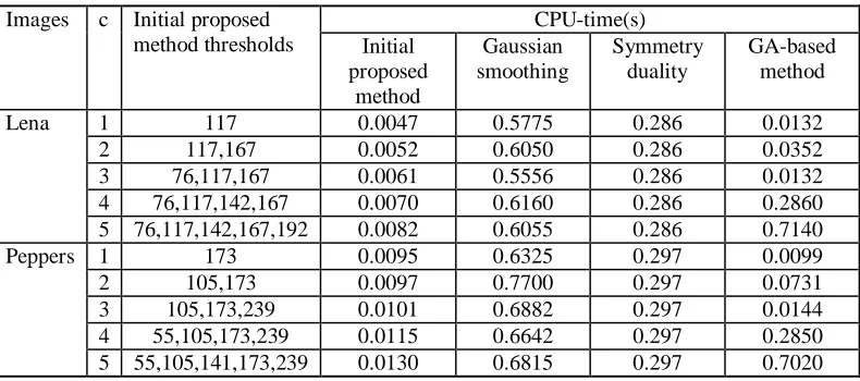
The complexity of this algorithm is the same as bi-level thresholding because all values in the range of [0, L-1] are examined for every new threshold. It means that bi-level thresholding algorithms are used for c times, if we want to find c thresholds. Thus the time complexity of the algorithm is O(c.n), which is a linear complexity. Table 1 compares the algorithm runtime with Gaussian-smoothing method, Symmetry-duality method, GA learning-Otsu method and PSO based method with c = 1 to 5 for Lena and Pepper images. As can be seen from Table 1, the CPU-time results of iterative initializing method are linear and quick.
Table 1. Time complexities of the proposed iterative initializing method, Gaussian-smoothing method, Symmetry-duality method and GA-based method
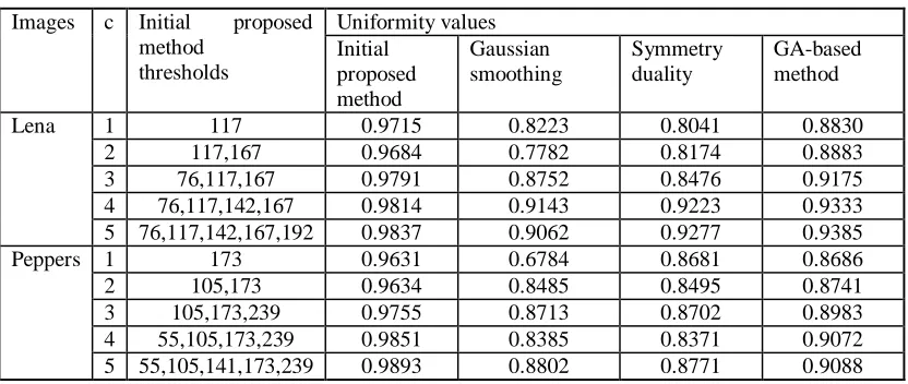
The uniformity values are also computed in Table 2. The results indicate that this initializing method is superior to other methods. From these results one can see that multi-level thresholding method gives a better result in nearly no time, so it can be considered a good choice for initializing thresholds.
Table 2. Uniformity values of the proposed iterative initializing method, Gaussian-smoothing method, Symmetry-duality method and GA-based method.
Uniformity values
Initial proposed
method thresholds c Images GA-based method Symmetry duality Gaussian smoothing Initial proposed method 0.8830 0.8041 0.8223 0.9715 117 1 Lena 0.8883 0.8174 0.7782 0.9684 117,167 2 0.9175 0.8476 0.8752 0.9791 76,117,167 3 0.9333 0.9223 0.9143 0.9814 76,117,142,167 4 0.9385 0.9277 0.9062 0.9837 76,117,142,167,192 5 0.8686 0.8681 0.6784 0.9631 173 1 Peppers 0.8741 0.8495 0.8485 0.9634 105,173 2 0.8983 0.8702 0.8713 0.9755 105,173,239 3 0.9072 0.8371 0.8385 0.9851 55,105,173,239 4 0.9088 0.8771 0.8802 0.9893 55,105,141,173,239 5
4. PROPOSED ABC MULTILEVEL THRESHOLDING ALGORITHM
Artificial Bee Colony (ABC) algorithm was developed by Karaboga for numerical optimization [ 21]. The inspiration behind this algorithm is the foraging behavior of honey bee swarms in finding foods. Some popular and well-known evolutionary algorithms such as Particle Swarm Optimization (PSO) and Genetic Algorithm (GA) have been compared with the ABC algorithm on some unconstrained and constrained problems [22-25]. The ABC algorithm is also applied on the clustering algorithms [ 26] and the training of neural networks [27, 28] with the proposed objective function in 29]. The previous studies showed that ABC outperforms other meta-heuristic algorithms on most of the engineering problems. ABC algorithm divides artificial bees into three groups of bees: employed, onlooker and scout bees. Employed bees bring their information about food sources for onlooker bees. This information is prepared for onlooker bees by dancing on dance area. From these dances, the onlookers could realize which source is better. Another type of bee which search the area stochastically, is the scout bee. The artificial bee colony is divided into equal parts. The first part includes the employed bees and the other part consists of the onlooker bees. If a food source is discarded by other bees, the employed bee which found that food source will turn into a scout bee. The pseudo-code of the ABC algorithm is presented in Fig. 2.
First, Psize food sources or solutions are initialized around the results which are found by the iterative method in the preprocessing section according to the following constraint, that the numbers should be ascending to not having overlap between segmented classes. Then employed and onlooker bees are produced where the number of bees in each group is equal to the food sources. Each food source in this algorithm indicates a solution for the optimization problem. The amount of nectar or the quality measure known as fitness is computed as follows:
1
1
i ifit
f
(16)_________________________________________________________________________________________ Initialization:
Generate a random population around the food sources suggested by iterative method location. Zi,i=1,…,Psize
//Psize denotes the size of population Compute fitness of the population as defined by (16)
Do
For each employed bee
Compute solution vi according to (17).
Compute the value of fi
Update food source if the new food source is more reliable.
End
Compute probability of food selection as specified by (18).
For every onlooker bee
Select a solution according to its probability.
Compute solution vi according to (19).
Compute the value of fi
Update food source if the new food source is more reliable.
End
If there is an abandoned food source for the scout
Replace solution with a new one as specified by (20).
Save the best solution up to now.
Until termination condition is met.
_____________________________________________________________________________________________
Fig. 2. The pseudocode of the proposed ABC algorithm for thresholding
The employed bees use their previous information and their current local information around them to update their locations if the quality of the found nectar is higher than their ex-locations. Flying Pattern of the employed bees is computed as follows from what is remembered before:
( )
ij ij ij ij kj v z
z z(17)
where j∈{1,2,...,D} and k ∈{1,2,..., Psize } denote indices which are chosen arbitrarily. Coefficient ij is chosen randomly between [−1, 1]. The fitness of vij is then compared with the previous food source fitness and if the recent one is better or equal to it, it is exchanged with the old one.
The employed bees return to their hive to share their information with the onlooker bees by some dancing styles, which demonstrate the direction and the amount of nectar in the food sources. The onlooker bees evaluate this information and choose to go to a food source according to some probability functions defined as follows:
1
size
i j P
n n
fit p
fit
(18)
where Psize is the number of food sources which is equal to the number of both employed bees and
onlooker bees, and fiti is given in Eq. (16).
The onlooker bees also used their memorized best food position and the newly chosen food source to
update their position if the quality of nectar is better than the previous memorized position. The onlooker
bees flying trajectories are updated as follow:
( )
ij ij ij ij wj v z
z z(19)
between [−1, 1]. The fitness of vij is then compared with the previous food source fitness and if the new one is better or equal to it, it is replaced with the old one.
The scout bees change a deserted food source with a haphazardly produced food source. If a food source position does not change after a predefined number of iteration called ‘limit’, it is assumed as deserted food source. If we presume that the deserted food source is zi then the update rule is defined as follows:
min (0,1)( max min)
j j j j
i
z z rand z z
(20) where j {1, 2, . . . , D}.
In ABC algorithm, the exploration is exerted by the employees and the onlooker in the search area and the scout bees in the search space do the exploitation.
5. EXPERIMENTAL RESULTS
This section presents the conducted experiments to evaluate the performance of the proposed algorithm on the well-known benchmarks.
a) Performance metric
The uniformity measure was proposed by Levine and Nazif 19] for measuring image segmentation quality. Next, Sahoo et al. [ 2] recommended using this measure to test the performance of thresholding algorithms. This quality measure corresponds to Otsu criterion measure [ 20]. The uniformity measure can be formulated as follows:
2
0
2 max min
(
)
1 2
(
)
j
c
i j j i R
f
U
c
N
f
f
(21)
where c denotes number of thresholds, Rj indicates the segmented region j, fi represents the gray level of pixel i, μj points to the mean of the gray levels of pixels in the segmented region j, N indicates the total number of pixels in the given image, fmax represents the maximum gray level of pixels in the given image, fmin demonstrates the minimum gray level of pixels in the given image.
The uniformity value is between 0 and 1. The higher values which are closer to 1 means that the quality of thresholding is better.
b) Settings of the algorithms
The performance of the proposed algorithm in comparison with the performances of Genetic Algorithm based multiple thresholding [ 30], Gaussian-smoothing method [10, 11] and Symmetry-duality method [9, 31] are presented in this section. Four well-known images (i.e. Lena, Peppers, House, and Elaine) are used here for comparison with other methods [ 14]. The benchmark images downloaded from 32] and [ 33] are of size 512×512.
c) Parameters tuning
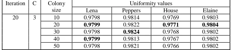
In the first experiment, the effect of the colony size is studied. The size of colony varies between 10 and 50 in steps of 10. In this experiment, parameter c is set at 3 and the number of iterations is fixed at 20. All the results are the average of 10 independent runs. Table 3 shows the performance of the proposed algorithm with a colony of different sizes. From Table 3, it can be seen that the size of the colony affects the performance of the proposed algorithm. It seems that the uniformity measures for a specific colony size of 20 could be the best choice with different number of iterations.
Table 3. Uniformity values for c = 3 and diverse colony size for four benchmark images
Uniformity values Colony
size C
Iteration
Elaine House
Peppers Lena
0.9803 0.9769
0.9814 0.9798
10 3
20
0.9804 0.9771
0.9822
0.9799
20
0.9802 0.9768
0.9824
0.9798 30
0.9802 0.9767
0.9813
0.9799
40
0.9802 0.9766
0.9821 0.9798
50
In the second experiment, the effect of the iteration numbers is studied. The number of iterations varies between 10 and 50 in steps of 10. In this experiment, parameter c is set equal to 3 and the size of the colony is fixed at 20. All the results are the average of 10 independent runs. Table 4 shows the performance of the proposed algorithm under different number of iterations. From Table 4, it can be seen that the number of iterations affects the performance of the proposed algorithm. The best results are obtained when the number of iterations is set at 20.
Table 4. Uniformity values for c = 3 and diverse iterations for four benchmark images
Uniformity values Iterations
C Colony
size Lena Peppers House Elaine
0.9801 0.9768
0.9825
0.9791 10
3 20
0.9804 0.9771
0.9824
0.9799
20
0.9802 0.9767
0.9824
0.9799
30
0.9801 0.9767
0.9820
0.9799
40
0.9801 0.9768
0.9821 0.9798
50
These results show that ABC algorithm has better performance with 20 iterations and a colony size
with 20 bees. We choose these parameters not only because of slight changes in the results, but the less computation time that we gain. This could make our proposed algorithm faster than the PSO based method since 100 iterations were used to converge to the optimum solution with 25 particles.
Coefficients did not affect the performance of the algorithm since they were uniformly generated in a fixed range.
d) Comparative study
Table 5.Uniformity values of the proposed ABC multilevel thresholding, PSO based method, Gaussian-smoothing, Symmetry-duality and GA-based method for Lena and Peppers images
Uniformity Values Proposed method thresholds c Images GA-based method Symmetry duality Gaussian smoothing PSO based method Proposed method 0.8883 0.8174 0.7782 0.9730 0.9726 96,156 2 Lena 0.9175 0.8476 0.8752 0.9503 0.9798 80,126,170 3 0.9333 0.9223 0.9143 0.9761 0.9835 74,115,147,179 4 0.9385 0.9277 0.9062 0.9828 0.9844 71,106,136,159,191 5 0.8741 0.8495 0.8485 0.9650 0.9740 103,192 2 Peppers 0.8983 0.8702 0.8713 0.9748 0.9820 68,132,202 3 0.9072 0.8371 0.8385 0.9738 0.9873 63,117,165,213 4 0.9088 0.8771 0.8802 0.9738 0.9892 55,104,142,174,220 5
The proposed method is also compared with basic PSO and adaptive PSO [14] for Elaine and House images. Table 6 presents the uniformity values of the proposed algorithm in comparison with PSO and adaptive PSO. The results show that the proposed method has competitive performance compared to the other methods. The best results on the House image for c=2 and c=3 are obtained by Adaptive PSO method. Except for these cases, the proposed method performs better on other cases.
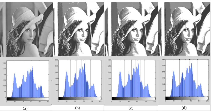
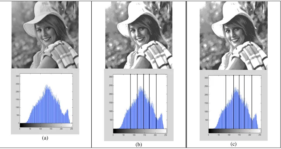
As mentioned before, the proposed algorithm is applied for Lena, Peppers, House and Elaine images and different thresholds are used to segment them. For other algorithms, the mentioned thresholds in their papers are used to represent segmented images. The results of hybrid GA, PSO and ABC, which are derived thresholds on the histogram of images and their corresponding images with thresholds are shown in Figs. 3-6.
In the previous works like Gaussian-smoothing and symmetry/duality methods, it can be seen that these methods tend to put threshold at the valley of histograms, which is the best for images with distinct foreground and background but population-based algorithms like PSO or GA can work with more complex histograms which may have unequal-size peaks or flat valleys [ 2]. These methods care more about the characteristics of images based on discriminant analysis, which can be seen in Figs. 3-6. As it can be seen in Fig. 3b, Fig. 4b, Fig. 5b the quality of images with thresholds is better than other images, but the quality of Fig. 6b and Fig. 6c are nearly the same as each other since the founded thresholds are nearly similar.
Table 6.Uniformity values of the proposed ABC multilevel thresholding, Adaptive PSO and basic PSO method for House and Elaine images
Uniformity values Proposed method
thresholds
c
Images Basic PSO
method Adaptive PSO based
(a) (b) (c) (d)
Fig. 3. Gray scale image and histogram of a) Original Lena b) Proposed Method c) Adaptive PSO d) GA for c=5 thresholds
(a) (b) (c) (d)
(a) (b) (c)
Fig. 5. Gray scale image and histogram of a) Original House b) Proposed Method c) Adaptive PSO for c=5 thresholds
6. CONCLUSION
In this study, we proposed a new optimal multilevel thresholding based on ABC algorithm and Otsu’s method. An iterative initializing method was also used to make the algorithm converge faster. This idea makes the computation complexity grow linearly when higher number of thresholds is selected. Owing to this property, this algorithm could be used in real situations. The results show that this method is superior to other well-known and popular methods proposed previously.
(a)
(b) (c)
REFERENCES
1. Sezgin, M. & Sankur, B. (2004), Survey over image thresholding techniques and quantitative performance evaluation.
Journal of Electronic Imaging, Vol. 13, pp. 146–165.
2. Sahoo, P. K., Soltani, S., Wong, A. K. C. & Chen, Y. C. (1988). A survey of thresholding techniques, ComputerVision Graphics Image Process, Vol. 41, pp. 233-260.
3. Lee, S. U., Chung, S. Y. & Park, R. H. (1990). A comparative performance study of several global thresholding techniques for segmentation, ComputerVision Graphics Image Process, Vol. 52, pp. 171—190.
4. Kapur, J. N., Sahoo, P. K. & Wong, A. K. C. (1985). A new method for gray-level picture thresholding using the entropy of the histogram. Computer Vision Graphics Image Processing, Vol. 2, pp. 273–285.
5. Kittler, J. & Illingworth, J. (1986). Minimum error thresholding. Pattern Recognition, Vol. 19, pp. 41–47.
6. Pun, T. (1981). Entropy thresholding: A new approach. Computer Vision Graphics Image Processing, Vol. 16, pp. 210–239.
7. Pun, T. (1980). A new method for grey-level picture thresholding using the entropy of the histogram. Signal Processing, Vol. 2, pp. 223–237.
8. Otsu, N. (1979). A threshold selection method from gray-level histograms. IEEE Transactions on Systems, Man, Cybernet, SMC-9, 62–66.
9. Yin, P. Y. & Chen, L. H. (1993). New method for multilevel thresholding using the symmetry and duality of the histogram.
Journal of Electronics and Imaging, Vol. 2, pp. 337–344.
10. Tsai, D. M. (1995). A fast thresholding selection procedure for multimodal and unimodal histograms. Pattern Recognition Letters, Vol. 16, pp. 653–666.
11. Lim, Y. K. & Lee, S. U. (1990). On the color image segmentation algorithm based on the thresholding and the fuzzy c-means techniques. Pattern Recognition, Vol. 23, pp. 935–952.
12. Yin, P. Y. & Chen, L. H. (1997). A fast iterative scheme for multi-level thresholding methods. Signal Processing 60, pp. 305-313.
13. Karaboga, D. (2005). An idea based on honey bee swarm for numerical optimization. Technical Report-TR06, Erciyes University, Engineering Faculty, Computer Engineering Department.
14. Chander, A., Chatterjee, A. & Siarry, P. (2011). A new social and momentum component adaptive PSO algorithm for image segmentation. Expert Systems with Applications, Vol. 38, Issue 5, pp. 4998–5004.
15. Akbari, R., Mohammadi, A. & Ziarati, K. (2010). A novel bee swarm optimization algorithm for numerical function optimization. Communications in Nonlinear Science and Numerical Simulation, Vol. 15, pp. 3142–3155.
16. Hatam, M. & Masnadi-Sirazi, M. A. (2008). Analytical discrete optimization. Iranian Journal of Science & Technology, Transaction B, Engineering, Vol. 32, No. B3, pp. 249-263.
17. Akbari, R. & Ziarati, K. (2011). A Cooperative approach to bee swarm optimization algorithm. Journal of Information Science and Engineering, Vol. 27, No. 3, pp. 799-818.
18. Niknam, T. & Golestaneh, F. (2012). Enhanced bee swarm optimization algorithm for dynamic economic dispatch. IEEE Systems Journal, DOI: 10.1109/JSYST.2012.2191831, Issue 99.
19. Levine, M. D. & Nazif, A. M. (1985). Dynamic measurement of computer generated image segmentations. IEEE Trans. Pattern Analysis and Machine Intelligence, Vol. 7, pp. 155-164.
20. Ng, W. S. & Lee, C. K. (1996). Comment on using the uniformity measure for performance measure in image segmentation.
IEEE Transactions on Pattern Analysis And Machine Intelligence, Vol. 18, No. 9.
21. Karaboga, D. (2005). An idea based on honey bee swarm for numerical optimization. Technical Report-TR06, Erciyes University, Engineering Faculty, Computer Engineering Department.
22. Basturk, B. & Karaboga, D. (2006). An artificial bee colony (ABC) algorithm for numeric function optimization. IEEE Swarm Intelligence Symposium, Indiana, USA.
24. Karaboga, D. & Basturk, B. (2007). A powerful and efficient algorithm for numerical function optimization: Artificial Bee Colony (ABC) algorithm. J. Global Optim. Vol. 39, Issue 3, pp. 171–459.
25. Akbari, R., Zeighami, V. & Ziarati, K. (2011). Artificial bee colony for resource constrained project scheduling problem.
International Journal of Industrial Engineering Computations, Vol. 2, No. 1, pp. 45-60.
26. Karaboga, D. & Ozturk, C. (2011). A novel clustering approach: Artificial Bee Colony (ABC) algorithm. Applied Soft Computing, Vol. 11, pp. 652–657.
27. Karaboga, D., Basturk, B. & Ozturk, C. (2007). Artificial Bee Colony (ABC) optimization algorithm for training feed-forward neural networks, LNCS: Modeling Decisions for Artificial Intelligence, MDAI. Vol. 4617, Springer–Verlag, pp. 318–329.
28. Karaboga, D. & Ozturk, C. (2009). Neural networks training by Artificial Bee Colony Algorithm on pattern classification.
Neural Network World, Vol. 19, Issue 3, pp. 279–292.
29. De Falco, I., Della Cioppa, A. & Tarantino, E. (2007). Facing classification problems with particle swarm optimization.
Journal of Applied Soft Computing, Vol. 7, Issue 3, pp. 652–658.
30. Yin, P. Y. (1999). A fast scheme for optimal thresholding using genetic algorithms. Signal Processing, Vol. 72, pp. 85–95
31. Yin, P. Y. & Chen, L. H. (1993). New method for multilevel thresholding using the symmetry and duality of the histogram.
Journal of Electronics and Imaging, Vol. 2, pp. 337–344
32. http://www.imageprocessingplace.com/root_files_V3/image_databases.htm