The Degree of an Edge in Union and Join of Two Fuzzy Graphs

(1)

Vol. 4, No. 1, 2014, 8-19

ISSN: 2320 –3242 (P), 2320 –3250 (online) Published on 17 March 2014

www.researchmathsci.org

8

International Journal of

The Degree of an Edge in Union and Join of Two Fuzzy

Graphs

K. Radha1 and N. Kumaravel2 1

P.G. Department of Mathematics, Periyar E.V.R College, Triuchrappalli – 620023 Tamilnadu, India. E-mail: [email protected]

2

Dept. of Mathematics, Paavai College of Engineering, Pachal, Namakkal – 637018 Tamil Nadu, India. E-mail: [email protected]

Received 27 February 2014; accepted 10 March 2014

Abstract. A fuzzy graph can be obtained from two given fuzzy graphs using union and join. In this paper, we find the degree of an edge in fuzzy graphs formed by these operations in terms of the degree of edges in the given fuzzy graphs in some particular cases.

Keywords: Degree of a vertex, degree of an edge, union and join. AMS Mathematics Subject Classification (2010): 03E72, 05C72 1. Introduction

Fuzzy graph theory was introduced by Azriel Rosenfeld in 1975 [4]. Though it is very young, it has been growing fast and has numerous applications in various fields. During the same time Yeh and Bang have also introduced various concepts in connectedness in fuzzy graphs [9]. Mordeson and Peng introduced the concept of operations on fuzzy graphs. Sunitha and Vijayakumar discussed about complementary of the operations of union, join, Cartesian product and composition on two fuzzy graphs [8]. The degree of a vertex in fuzzy graphs which are obtained from two given fuzzy graphs using these operations were discussed by Nagoor Gani and Radha [3]. Radha and Kumaravel introduced the concept of degree of an edge and total degree of an edge in fuzzy graphs [5]. We study about the degree of an edge in fuzzy graphs which are obtained from two given fuzzy graphs using the operations of union and join. In general, the degree of an edge in union and join of two fuzzy graphs G1 and G2 cannot be expressed in terms of these in G1 and G2. In this paper, we find the degree of an edge in union and join of two fuzzy graphs G1 and G2 in terms of the degree of edges of G1 and G2 in some particular cases.

First we go through some basic concepts.

(2)

9

Throughout this paper, G1: (σ1, µ1) and G2: (σ2, µ2) denote two fuzzy graphs with underlying crisp graphs G1

*

: (V1, E1) and G2 *

: (V2, E2) with |Vi| = pi, i = 1, 2. Also

) (

* i G u d

i denotes the degree of ui in Gi *

.

Definition 1.2. [3] Let G: (σ, µ) be a fuzzy graph on G*: (V, E). The degree of a vertex u is dG(u) =

∑

≠v u

uv)

(

µ

=

∑

∈E uv

uv)

(

µ

.

The minimum degree of G is δ(G) = ∧{dG(v) : v ∈ V}. The maximum degree of G is ∆(G) = ∨{dG(v) : v ∈ V}.

Definition 1.3. [3] The total degree of a vertex u∈ V is defined by tdG(u) =

∑

≠v u

uv)

(

µ

+ σ(u) = dG(u) + σ(u).

Definition 1.4. [1] Let G*: (V, E) be a graph and let e = uv be an edge in G*. Then the degree of an edge e = uv∈ E is defined by dG*(uv) = dG*(u) + dG*(v) – 2.

Definition 1.5. [3] Let G1: (σ1, µ1) and G2: (σ2, µ2) be two fuzzy graphs with underlying graphs G1*: (V1, E1) and G2*: (V2, E2) and let G* = G1*∪ G2* = (V1 ∪ V2, E1 ∪ E2) be the union of G1

* and G2

*

. Then the union of two fuzzy graphs G1 and G2 is a fuzzy graph G = G1∪ G2: (σ1∪σ2, µ1∪µ2) defined by

(σ1∪σ2)(u) =

   

∩ ∈ ∨

−

∈ −

∈

2 1 2

1

1 2 2

2 1 1

), ( ) (

), (

V V u if u u

V V u if u

σ

(µ1∪µ2)(uv) =

   

∩ ∈ ∨

−

∈∈ −

2 1 2

1

1 2 2

2 1 1

), ( ) (

), (

E E uv if uv uv

E E uv if uv

µ

.

Definition 1.6. [3] Let G1: (σ1, µ1) and G2: (σ2, µ2) be two fuzzy graphs with underlying graphs G1*: (V1, E1) and G2*: (V2, E2) with V1∩ V2 = φ and let G* = G1* + G2* = (V1 ∪ V2, E1 ∪ E2∪ E′) be the join of G1

*

and G2 *

, where E′ is the set of all edges joining the vertices of V1 and V2. Then the join(sum) of two fuzzy graphs G1 and G2 is a fuzzy graph G = G1 + G2: (σ1 + σ2, µ1 + µ2) defined by

(σ1 + σ2)(u) = (σ1∪σ2)(u), ∀ u ∈ V1 ∪ V2 and

(µ1 + µ2)(uv) =

  

′ ∈ ∧

∪ ∈ ∪

E uv if v u

E E uv if uv

), ( ) (

), )( (

2 1

2 1 2

1

σ

(

µ

+

∑

≠∈u w

E wv

wv)

(

µ

.

The minimum degree of G is δE(G) = ∧{dG(uv) : uv∈ E}. The maximum degree of G is ∆E(G) = ∨{dG(uv) : uv∈ E}.

Definition 1.10. [5] Let G: (σ, µ) be a fuzzy graph on G*: (V, E). The total degree of an edge uv∈ E is defined by tdG(uv) = dG(uv) + µ(uv) = dG(u) + dG(v) – µ(uv).

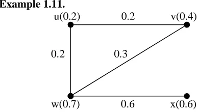
Example 1.11.

u(0.2) 0.2 v(0.4)

0.2 0.3

w(0.7) 0.6 x(0.6)

Figure 1.1. Fuzzy graph G: (σ, µ)

dG(u) = µ(uv) + µ(uw) = 0.2 + 0.2 = 0.4, tdG(u) = dG(u) + σ(u) = 0.4 + 0.2 = 0.6.

δ(G) = ∧{dG(v), ∀ v∈V} = ∧{0.4, 0.5, 1.1, 0.6} = 0.4 = dG(u). ∆(G) = ∨{dG(v), ∀ v∈V} = ∨{0.4, 0.5, 1.1, 0.6} = 1.1 = dG(w). dG(uv) =

∑

≠∈v w

E uw

uw)

(

µ

+

∑

≠∈u w

E wv

wv)

(

µ

= 0.2 + 0.3 = 0.5.

tdG(uv) = dG(uv) + µ(uv) = 0.5 + 0.2 = 0.7.

δE(G) = ∧{dG(uv), ∀uv∈E} = ∧{0.5, 1.1, 1.0, 0.5} = 0.5 = dG(uv) = dG(wx). ∆E(G) = ∨{dG(uv), ∀uv∈E} = ∨{0.5, 1.1, 1.0, 0.5} = 1.1 = dG(uw).

2. Degree of an edge in union

For anyuv∈E1∪E2, fix u∈V1∪V2. We have three cases to consider. Case 1: V1∩ V2 = φ.

Let uv ∈ E1∪ E2 be any edge. Hence E1∩ E2= φ.

(4)

11 So (µ1∪µ2)(uv) =

  

− ∈

1 2 2

2 1 1

), (

E E uv if uv

µ

.

By definition, ( )

2 1 uv

d_G_∪_G =

∑

≠ ∪ ∈

≠ ∈E wu wv

wv ,

1 1

) (

µ

.

∴ ( )

2 1 uv

dG∪G = dG₁(uv).

Similarly, if uv∈ E2, ( ) 2 1 uv

dG∪G = dG₂(uv).

Example 2.1.

u(0.5) x(0.4)

0.3 0.4 0.3

w(0.4) 0.4 v(0.6) z(0.6) 0.5 y(0.7) G1 G2

u(0.5) x(0.4)

0.3 0.4 0.3

w(0.4) 0.4 v(0.6) z(0.6) 0.5 y(0.7)

G1∪∪∪∪ G2 Figure 2.1:

Here uv ∈ E1. Then ( ) 2 1 uv

dG∪G = dG₁(uv) = 0.3 + 0.4 = 0.7. Case 2: V₁∩V₂ ≠

φ

, E₁∩E₂ =

φ

.

Then uv∈E₁ or uv∈E₂. Choose uv∈E₁. Then uv∉E₂. Also, if both u,v∉V1∩V2, then it is of case 1.

So, consider either u∈V1∩V2 or v∈V1∩V2 or both u,v∈V1∩V2. Subcase 1: u∈V₁∩V₂ or v∈V₁∩V₂.

When u∈V₁∩V₂, By definition, ( )

2 1 uv

dG∪G = dG₁∪G₂(u)+dG₁∪G₂(v)−2(

µ

1∪

µ

2)(uv). = [ ( ) ( )] ( ) 2 ₁( )

1 2

1 u d u d v uv

d_G + _G + _G −

µ

.

= [ ( ) ( ) 2 ( )] ( )

2 1

1 u d v 1 uv d u

dG + G −

µ

+ G .

∴ ( )

2 1 uv

(5)

12

Similarly, ( )

2 1 uv

d_G_∪_G = ( ) ( )

2 1 uv d v

d_G + _G , if v ∈ V1∩ V2.

Thus,

  

∩ ∈ +

=

∪

2 1

), ( ) (

), ( ) ( )

(

2 1

2

1 _d _uv _d _v _if_v _V _V

V V u if u d uv d uv d

G G

G

G _.

In a similar way, if uv∈E₂, then

  

∩ ∈ +

=

∪

2 1

), ( ) (

), ( ) ( )

(

1 2

2

1 _d _uv _d _v _if _v _V _V

V V u if u d uv d uv d

G G

G

G _.

Example 2.2.

u(0.5) u(0.4)

0.3 0.4 0.3

w(0.4) 0.4 v(0.6) x(0.6) 0.5 y(0.7) G1 G2

u(0.5)

0.3 0.4 0.3

w(0.4) 0.4 v(0.6) x(0.6) 0.5 y(0.7)

G1∪∪∪∪ G2

Figure 2.2:

Here uv∈E₁ and u∈V₁∩V₂. Then dG₁∪G₂(uv) = dG1(uv)+dG2(u) = 0.7 + 0.3 = 1.0.

Subcase 2: u,v∈V₁∩V₂, uv∈E₁.

Since E₁∩E₂ =

φ

, no edge incident at u or v is in E₁∩E₂.

Since the edges incident at u & v in G₁and also in G₂ appear with the same membership values in G₁∪G₂.

By definition, ( )

+ _G + _G .

∴ ( )

2 1 uv

dG∪G = dG₁(uv)+dG₂(u)+dG₂(v).

In a similar way, if uv∈E2, then dG₁∪G₂(uv) = dG₂(uv)+dG₁(u)+dG₁(v).

(6)

13

u(0.5) u(0.4) u(0.5)

0.3 0.4 0.3 0.3 0.4 0.3

w(0.4) 0.4 v(0.6) x(0.6) 0.5 v(0.7) w(0.4) 0.4 v(0.7) 0.5 x(0.6) G1 G2 G1∪∪∪∪ G2

Figure 2.3:

Here uv∈E₁ and u,v∈V₁∩V₂. Then ( )

2 1 uv

dG∪G = dG₁(uv)+dG₂(u)+dG₂(v) = 0.7 + 0.3 + 0.5 = 1.5.

Case 3: V₁∩V₂ ≠

φ

, E₁∩E₂ ≠

φ

.

Then uv∈E1∩E2. Therefore uv∈E1 and uv∈E2.

So, consider either no edge incident at u & v other than uv is in E1∩E2 or some of the edges incident at u & v other than uv are in E₁∩E₂.

Subcase 1: No edge incident at u and v other than uv is in E₁∩E₂.

Then the edge incident at u or v is in either E1 or in E2, those edges appear with the same membership value in G1∩G2.

By definition,

) (

2 1 uv

d_G_∪_G =

∑

≠ ∪ ∈

∪

v w E E uw

uw ,

2 1 2 1

) )(

(

µ

+

∑

≠ ∪ ∈

∪

u w E E wv

wv ,

2 1 2 1

) )( (

µ

.

=

∑

≠ −

∈E E w v

.

=

∑

≠ −

∈E E w v

+

∑

≠ −

∈E E w u

wv

wv ,

2 1 2

) (

µ

.

∴ ( )

2 1 uv

d_G_∪_G = ( )

1 uv

d_G + ( )

2 uv d_G .

Example 2.4.

u(0.5) u(0.4) u(0.5)

0.3 0.4 0.3 0.3 0.4

w(0.4) 0.4 v(0.6) v(0.6) 0.5 y(0.7) w(0.4) 0.4 v(0.6) 0.5 y(0.7) G1 G2 G1∪∪∪∪ G2

Figure 2.4: Here uv ∈ E1∩ E2.

Then ( )

2 1 uv

dG∪G = dG₁(uv) + dG₂(uv) = 0.7 + 0.5 = 1.2.

(7)

14 By definition, ( )

2 1 uv

. ∴ ( ) 2 1 uv

dG∪G = dG₁(uv) + dG2(uv) –

∑

≠ ∩ ∈ ∧ v w E E uw uw uw , 2 1 2 1 ) ( ) (

µ

–

∑

≠ ∩ ∈ ∧ u w E E wv wv wv , 2 1 2 1 ) ( ) (

µ

. Example 2.5.

u(0.5) 0.4 x(0.6) u(0.4) 0.3 x(0.5) u(0.5) 0.4 x(0.6)

0.3 0.4 0.3 0.3 0.4

w(0.4) 0.4 v(0.6) v(0.6) 0.5 y(0.7) w(0.4) 0.4 v(0.6) 0.5 y(0.7) G1 G2 G1∪∪∪∪ G2

Figure 2.5: Here uv ∈ E1∩ E2.

Then ( )

2 1 uv

(8)

15 ∴ ( )

2 1 uv

dG∪G = 1.1 + 0.8 – 0.3 – 0 = 1.6.

3. Degree of an edge in join

Here V1∩ V2 = φ. Hence E1∩ E2 = φ.

(µ1 + µ2)(uv) =

    ′ ∈ ∧ ∈ ∈ E uv if v u E uv if uv E uv if uv ), ( ) ( ), ( ), ( 2 1 2 2 1 1

σ

µ

By definition, ( ) 2 1 uv

dG+G =

∑

≠ ′ ∪ ∪

∈E E E w v

uw uw , 2 1 ) (

µ

+

∑

≠ ′ ∪ ∪

∈E E E w u

wv wv , 2 1 ) (

µ

.

i.e., ( )

2 1 uv

. ∴ ( ) 2 1 uv

dG+G = dG₁(uv) +

∑

′ ∈ ∧ E uw w

u) ( )

( ₂ 1

σ

+

∑

′ ∈ ∧ E vw w

v) ( )

( ₂

1

σ

(4.1)

Similarly, for any uv∈ E2,

dG1+G2(uv) = dG2(uv) +

∑

′ ∈ ∧ E wu u

w) ( )

( ₂ 1

σ

+

∑

′ ∈ ∧ E wv v

w) ( )

( ₂

1

σ

(4.2)

and for any uv∈ E′ with u ∈ V1, v ∈ V2,

( )

2 1 uv

Theorem 3.2. Let G1: (σ1, µ1) and G2: (σ2, µ2) be two fuzzy graphs. 1. If σ1≥σ2, then

( )

2 1 uv dG+G =

(9)

16 2. If σ2≥σ1, then

( )

2 1 uv dG+G =

    

′ ∈ −

+ +

+

∈ +

+

E uv if u p

G O v d u d

E uv if G

O uv d

E uv if v

u p uv d

G G

), ( ) 2 ( ) ( ) ( ) (

), ( 2 ) (

)), ( ) ( ( ) (

1 2 1

2 1

1 1

1 2

2 1

σ

.

Proof. We have σ1≥σ2. From (4.1), for any uv∈ E1,

) (

2 1 uv

dG+G = dG₁(uv) +

∑

′ ∈

∧

E uw

w

u) ( )

( 2

1

σ

+

∑

′ ∈

∧

E vw

w

v) ( )

( 2

1

σ

= ( )

1 uv

′ ∈

∧

E wu

u

w) ( )

( 2

1

σ

+

∑

′ ∈

∧

E wv

v

w) ( )

( 2

1

σ

= ( )

2 uv

d_G +

∑

∈1

) (

2 V w

u

σ

+

∑

∈1

) (

2 V w

v

σ

∑

≠ ′ ∈

∧

u w E wv

v w

,

2 1( )

σ

( )

σ

= ( )

1 u

d_G + ( )

2 v

d_G +

∑

∈2

) (

2 V w

v1(0.5) v2(0.7) v1(0.5) 0.5 v2(0.7) G1 G2 G1 + G2

Figure 3.1: We have σ2≥σ1. So by (2) of theorem 3.2,

) ( 1 1 2 1 uv

(10)

17

) ( 2 2 2 1 u v

dG+G = dG₂(u2v2)+2O(G1) = 0 + 2(0.9) = 1.8

) ( 1 2 2 1 uv

dG+G = dG₁(u1)+dG₂(v2)+O(G1)+(p2−2)

σ

1(u1) = 0.3 + 0.4 + 0.9 + (2 – 2)(0.4) = 1.6.

The above degrees can be verified in the figure of G1 + G2 given in figure 3.1.

Theorem 3.4. Let G1: (σ1, µ1) and G2: (σ2, µ2) be two fuzzy graphs such that σ1 ∧σ2 is a constant function.

Then ( )

2 1 uv d_G₊_G =

    

′ ∈ −

+ + +

∈ +

E uv if p

p c v d u d

E uv if cp

uv d

E uv if cp

uv d

G G

), 2 (

) ( ) (

, 2 ) (

2 1

1 2

2 1

′ ∈

∧

E uw

w

u) ( )

( 2

1

σ

+

∑

′ ∈

∧

E vw

w

v) ( )

( 2

1

σ

= ( )

1 uv

d_G +

∑

∈

∧

2

) ( )

( 2

1 V w

w

u

σ

+

∑

∈

∧

2

) ( )

( 2

1 V w

w

v

σ

= ( )

1 uv

d_G +

∑

∈V2 w

c +

∑

∈V2 w

c

= ( )

1 uv

dG + cp2 + cp2

= ( )

1 uv

dG +2cp2. From (4.2), for any uv∈ E2, ( )

2 1 uv

d_G₊_G = ( )

2 uv

d_G +

∑

′ ∈

∧

E wu

u

w) ( )

( 2

1

σ

+

∑

′ ∈

∧

E wv

v

w) ( )

( 2

1

σ

= ( )

2 uv

d_G +

∑

∈V1 w

c +

∑

∈V1 w

c

= ( )

2 uv

dG + cp1 + cp1

= ( )

2 uv

dG + 2cp1.

From (4.3), for any uv∈ E′ with u ∈ V1 and v ∈ V2. ( )

2 1 uv

dG+G =dG₁(u)+dG₂(v)+

∑

≠ ′ ∈

∧

v w E uw

w u

,

2 1( )

σ

( )

σ

∧

−

+

∑

∈

= ( )

1 u

dG +dG₂(v)+p2c+ p1c−2c

= ( )

1 u

dG +dG₂(v)+c(p1+ p2−2).

(11)

18

u1(0.5) u2(0.4) u1(0.5) 0.4 u2(0.4)

0.4

0.3 0.2 0.3 0.2 0.4

v1(0.6) v2(0.4) v1(0.6) 0.4 v2(0.4) G1 G2 G1 + G2

Figure 3.2: By theorem 3.4,

(1). dG₁+G₂(u1v1) = dG₁(u1v1)+2cp2 = 0 + 2(0.4)(2) = 1.6 (2). dG₁+G₂(u2v2) = dG₂(u2v2)+2cp1 = 0 + 2(0.4)(2) = 1.6 (3). dG₁+G₂(u1v2) = dG₁(u1)+dG₂(v2)+c(p1+ p2 −2)

= 0.3 + 0.2 + 0.4(2 + 2 – 2) = 1.3

4. Conclusion

In this paper, we have found the degree of edges in G1∪ G2 in terms of G1 and G2, the degree of edges in G1 + G2 in terms of the degree of vertices and edges in G1 and G2 and also in terms of the degree of vertices in G1* and G2* under some conditions and illustrated them through examples. They will be more helpful especially when the graphs are very large. Also they will be useful in studying various conditions, properties of union and join of two fuzzy graphs.

REFERENCES

1. S. Arumugam and S. Velammal, Edge domination in graphs, Taiwanese Journal of Mathematics, 2(2) (1998) 173 – 179.

2. A.Nagoorgani and J.Malarvizhi, Properties of µ-complement of a fuzzy graph, Intern. J. Algorithms, Computing and Mathematics, 2(3) (2009) 73 – 83.

3. A. Nagoorgani and K. Radha, The degree of a vertex in some fuzzy graphs, Intern. J. Algorithms, Computing and Mathematics, 2(3) (2009) 107 – 116.

4. A. Rosenfeld, Fuzzy graphs, in: L.A. Zadeh, K.S. Fu, K. Tanaka and M. Shimura, (editors), Fuzzy sets and their applications to cognitive and decision process, Academic press, New York, (1975) 77 – 95.

5. K. Radha and N. Kumaravel, The degree of an edge in Cartesian product and composition of two fuzzy graphs, Intern. J. Applied Mathematics & Statistical Sciences, 2(2) (2013) 65 – 78.

6. H. Rashmanlou and M. Pal, Isometry on interval-valued fuzzy graphs,

(12)

19

7. M.S. Sunitha and Sunil Mathew, A survey of fuzzy graph theory, Annals of

Pure and Applied Mathematics, 4(1) (2013) 92 – 110.

8. M.S. Sunitha and A. Vijayakumar, Complement of a fuzzy graph, Indian Journal of Pure and Applied Mathematics, 33(9) (2002) 1451 – 1464.