Probabilistic Preference Learning with the Mallows Rank
Model
Valeria Vitelli [email protected]
Oslo Centre for Biostatistics and Epidemiology, Department of Biostatistics, University of Oslo, P.O.Box 1122 Blindern, NO-0317, Oslo, Norway
Øystein Sørensen [email protected]
Oslo Centre for Biostatistics and Epidemiology, Department of Biostatistics, University of Oslo, P.O.Box 1122 Blindern, NO-0317, Oslo, Norway
Marta Crispino [email protected]
Department of Decision Sciences, Bocconi University, via R¨ontgen 1, 20100, Milan, Italy
Arnoldo Frigessi [email protected]
Oslo Centre for Biostatistics and Epidemiology, University of Oslo and Oslo University Hospital, P.O.Box 1122 Blindern, NO-0317, Oslo, Norway
Elja Arjas [email protected]
Oslo Centre for Biostatistics and Epidemiology, Department of Biostatistics, University of Oslo, P.O.Box 1122 Blindern, NO-0317, Oslo, Norway
Editor:Francois Caron
Abstract
Ranking and comparing items is crucial for collecting information about preferences in many areas, from marketing to politics. The Mallows rank model is among the most successful approaches to analyze rank data, but its computational complexity has limited its use to a particular form based on Kendall distance. We develop new computationally tractable methods for Bayesian inference in Mallows models that work with any right-invariant dis-tance. Our method performs inference on the consensus ranking of the items, also when based on partial rankings, such as top-k items or pairwise comparisons. We prove that items that none of the assessors has ranked do not influence the maximum a posteriori con-sensus ranking, and can therefore be ignored. When assessors are many or heterogeneous, we propose a mixture model for clustering them in homogeneous subgroups, with cluster-specific consensus rankings. We develop approximate stochastic algorithms that allow a fully probabilistic analysis, leading to coherent quantifications of uncertainties. We make probabilistic predictions on the class membership of assessors based on their ranking of just some items, and predict missing individual preferences, as needed in recommendation systems. We test our approach using several experimental and benchmark data sets.
Keywords: Incomplete rankings, Pairwise comparisons, Preference learning with
uncer-tainty, Recommendation systems, Markov Chain Monte Carlo
c
1. Introduction
Various types of data have ranks as their natural scale. Companies recruit panels to rank novel products, market studies are often based on interviews where competing services or items are compared or ranked. In recent years, analyzing preference data collected over the internet (for example, movies, books, restaurants, political candidates) has been receiving much attention, and often these data are in the form of partial rankings.
Some typical tasks for rank or preference data are: (i) aggregate, merge, summarize multiple individual rankings to estimate the consensus ranking; (ii) predict the ranks of unranked items at individual level; (iii) partition the assessors into classes, each sharing a consensus ranking of the items, and classify new assessors to a class. In this paper we phrase all these tasks (and their combinations) in a unified Bayesian inferential setting, which allows us to also quantify posterior uncertainty of the estimates. Uncertainty evaluations of the estimated preferences and class memberships are a fundamental aspect of information in marketing and decision making. When predictions are too unreliable, actions based on these might better be postponed until more data are available and safer predictions can be made, so as not to unnecessarily annoy users or clients.
is driven by expectation propagation approximate inference, and scales to very large data sets without requiring strong factorization assumptions. Among probabilistic approaches,
Meilˇa and Chen (2010) use Dirichlet process mixtures to perform Bayesian clustering of
assessors in the Mallows model, but they again focus on the Kendall distance only. Jacques and Biernacki (2014) also propose clustering based on partial rankings, but in the context of the Insertion Sorting Rank (ISR) model. Hence, the approach is probabilistic but it is far from the general form of the Mallows, even though it has connections with the Mal-lows with Kendall distance. See Section 5 for a more detailed presentation of related work. For the general background on statistical methods for rank data, we refer to the excellent monograph by Marden (1995), and to the book by Alvo and Yu (2014).
The contributions of this paper are summarized as follows. We develop a Bayesian framework for inference in Mallows models that works with any right-invariant metric. In particular, the method is able to handle some of the right-invariant distances poorly con-sidered in the existing literature, because of their well-known intractability. In this way the main advantage of the Mallows models, namely its flexibility in the choice of the distance, is fully exploited. We propose a Metropolis-Hastings iterative algorithm, which converges to the Bayesian posterior distribution, if the exact partition function is available. In case the exact partition function is not available, we propose to approximate it using an off-line importance sampling scheme, and we document the quality and efficiency of this approx-imation. Using data augmentation techniques, our method handles incomplete rankings,
like the important cases of top-krankings, pairwise comparisons, and ranks missing at
ran-dom. For the common situation when the pool of assessors is heterogeneous, and cannot be assumed to share a common consensus, we develop a Bayesian clustering scheme which embeds the Mallows model. Our approach unifies clustering, classification and preference prediction in a single inferential procedure, thus leading to coherent posterior credibility levels of learned rankings and predictions. The probabilistic Bayesian setting allows us to naturally compute complex probabilities of interest, like the probability that an item has consensus rank higher than a given level, or the probability that the consensus rank of an item is higher than that of another item of interest. For incomplete rankings this can be done also at the individual assessor level, allowing for individual recommendations.
cluster-specific consensus rankings. Section 4.4 is dedicated to prediction in a realistic setup, which requires both the cluster assignment and personalized preference learning. We show that our approach works well in a simulation context. In Section 5 we review related methods which have been proposed in the literature, and compare by simulation some algorithms with our procedure (Section 5.1). In Section 6, we then move to the illustration of the performance of our method on real data: the selected case studies illustrate the different incomplete data situations considered. This includes the Sushi (Section 6.3) and Movielens (Section 6.4) benchmark data. Section 7 presents some conclusions and extensions.
2. A Bayesian Mallows Model for Complete Rankings
Assume we have a set of n items, labelled A = {A1, A2, . . . , An}. We first assume that
each of N assessors ranks all items individually with respect to a considered feature. The
ordering provided by assessorj is represented by Xj, whose ncomponents are items inA.
The item with rank 1 appears as the first element, up to the item with rank n appearing
as then-th element. The observationsX1, . . . ,XN are henceN permutations of the labels
inA. Let Rij =X−j1(Ai), i= 1, . . . , n, j= 1, . . . , N, denote the rank given to item Ai by
assessor j, and let Rj = (R1j, R2j, . . . , Rnj), j = 1, . . . , N, denote the ranking (that is the
full set of ranks given to the items), of assessorj. LettingPn be the set of all permutations
of {1, . . . , n}, we have Rj ∈ Pn, j = 1, . . . , N. Finally, let d(·,·) :Pn× Pn → [0,∞) be a
distance function between two rankings.
The Mallows model (Mallows, 1957) is a class of non-uniform joint distributions for a
ranking ronPn, of the formP(r|α,ρ) =Zn(α,ρ)−1exp{−(α/n)d(r,ρ)}1Pn(r), where ρ∈
Pnis the latent consensus ranking,αis a scale parameter, assumed positive for identification
purposes, Zn(α,ρ) = Pr∈Pne
−α
nd(r,ρ) is the partition function, and 1S(·) is the indicator
function of the setS. We assume that theNobserved rankingsR1, . . . ,RN are conditionally
independent givenα and ρ, and that each of them is distributed according to the Mallows
model with these parameters. The likelihood takes then the form
P(R1, . . . ,RN|α,ρ) =
1
Zn(α,ρ)N
exp
−α
n
N X
j=1
d(Rj,ρ)
N Y
j=1
{1Pn(Rj)}. (1)
For a given α, the maximum likelihood estimate of ρis obtained by computing
argmax
ρ∈Pn
exp n
−αnPN
j=1d(Rj,ρ)
o
Zn(α,ρ)N
. (2)
For largenthis optimization problem is not feasible, because the space of permutations has
n! elements. This has impact both on the computation ofZn(α,ρ),and on the minimization
of the sum in the exponential of (2), which is typically NP-hard (Bartholdi et al., 1989).
2.1 Distance Measures and Partition Function
Right-invariant distances (Diaconis, 1988) play an important role in the Mallows models. A right-invariant distance is unaffected by a relabelling of the items, which is a
d(ρ1ρ−21,1n), where 1n = {1,2, ..., n}, and therefore the partition function Zn(α,ρ) of
(1) is independent on the latent consensus ranking ρ. We write Zn(α,ρ) = Zn(α) =
P
r∈Pnexp{−
α
nd(r,1n)}. All distances considered in this paper are right-invariant.
Im-portantly, since the partition function Zn(α) does not depend on the latent consensus ρ,
it can be computed off-line over a grid for α, given n (details in Section 3). For some
choices of right-invariant distances, the partition function can be analytically computed. For this reason, most of the literature considers the Mallows model with Kendall distance
(Lu and Boutilier, 2014; Meilˇa and Chen, 2010), for which a closed form of Zn(α) is given
in Fligner and Verducci (1986), or with the Hamming (Irurozki et al., 2014) and Cayley (Irurozki et al., 2016b) distances. There are important and natural right-invariant distances for which the computation of the partition function is not feasible, in particular the footrule
(l1) and the Spearman’s (l2) distances. For precise definitions of all distances involved in
the Mallows model we refer to Marden (1995). Following Irurozki et al. (2016a), Zn(α)
can be written in a more convenient way. Since d(r,1n) takes only the finite number of
discrete valuesD={d1, ..., da}, whereadepends onnand on the distanced(·,·), we define
Li ={r∈ Pn:d(r,1n) =di} ⊂ Pn, i= 1, ..., a, to be the set of permutations at the same
given distance from1n, and |Li|corresponds to its cardinality. Then
Zn(α) = X
di∈D
|Li|exp{−(α/n)di}. (3)
In order to compute Zn(α) one thus needs |Li|, for all values di ∈ D. In the case of
the footrule distance, the set D includes all even numbers, from 0 to bn2/2c, and |L
i|
corresponds to the sequence A062869 available for n≤50 on the On-Line Encyclopedia of
Integer Sequences (OEIS) (Sloane, 2017). In the case of Spearman’s distance, the set D
includes all even numbers, from 0 to 2 n3
, and |Li| corresponds to the sequence A175929
available for n≤ 14 in the OEIS. When the partition function is needed for larger values
of n, we suggest an importance sampling scheme which efficiently approximates Zn(α) to
an arbitrary precision (see Section 3). An interesting asymptotic approximation for Zn(α),
when n→ ∞, has been studied in Mukherjee (2016), and we apply it in an example where
n= 200 (see Section 6.4, and Section 2 in the Supplementary Material).
2.2 Prior Distributions
To complete the specification of the Bayesian model for the rankings R1, . . . ,RN, a prior
for its parameters is needed. We assume a priori thatα and ρ are independent.
An obvious choice for the prior forρin the context of the Mallows likelihood is to utilize
the Mallows model family also in setting up a prior for ρ, and let π(ρ) = π(ρ|α0,ρ0) ∝
exp
−α0
nd(ρ,ρ0) . Here α0 and ρ0 are fixed hyperparameters, with ρ0 specifying the
ranking that is a priori thought most likely, and α0 controlling the tightness of the prior
around ρ0. Since α0 is fixed, Zn(α0) is a constant. Note that combining the likelihood
with the priorπ(ρ|α0,ρ0) above has the same effect on inference as involving an additional
hypothetical assessor j = 0, say, who then provides the ranking R0 =ρ0 as data, with α0
fixed.
If we were to elicit a value for α0, we could reason as follows. Consider, forρ0 fixed, the
of the distance d(·,·), this expectation is independent of ρ0, which is why gn(·) depends
only onα0. Moreover,gn(α0) is obviously decreasing inα0. For the footrule and Spearman
distances, which are defined as sums of item specific deviations |ρ0i −ρi| or |ρ0i −ρi|2,
gn(α0) can be interpreted as the expected (average, per item) error in the prior ranking
π(ρ|α0,ρ0) of the consensus. A value for α0 is now elicited by first choosing a target level
τ0, say, which would realistically correspond to such an a priori expected error size, and then
finding the value α0 such that gn(α0) =τ0. This procedure requires numerical evaluation
of the function gn(α0) over a range of suitable α0 values. In this paper, we employ only
the uniform prior π(ρ) = (n!)−11Pn(ρ) in the space Pn of n−dimensional permutations,
corresponding toα0= 0.
For the scale parameter α we have in this paper used a truncated exponential prior,
with density π(α|λ) =λe−λα1[0,αmax](α)/(1−e
−λαmax), where the cut-off point αmax <∞
is large compared to the values supported by the data. In practice, in the computations
involving sampling of values for α, truncation was never applied. We show in Figure 3 of
Section 3.3 on simulated data, that the inferences onρ are almost completely independent
of the choice of the value ofλ. Also a theoretical argument for this is provided in that same
section, although it is tailored more specifically to the numerical approximations of Zn(α).
For these reasons, in all our data analyses, we assigned λ a fixed value. We chose values
for λ close to 0, depending on the complexity of the data, thus implying a prior density
for α which is quite flat in the region supported in practice by the likelihood. If a more
elaborate elicitation of the prior forαfor some reason were preferred, this could be achieved
by computing, by numerical integration, values of the functionEπ(α)(gn(α)|λ), selecting a
realistic targetτ, and solving Eπ(α)(gn(α)|λ) =τ forλ. In a similar fashion as earlier, also
Eπ(α)(gn(α)|λ) can be interpreted as an expected (average, per item) error in the ranking,
but now by errors is meant those made by the assessors, relative to the consensus, and
expectation is with respect to the priorπ(α|λ).
2.3 Inference
Given the prior distributions π(ρ) and π(α), and assuming prior independence of these
variables, the posterior distribution for ρand α is given by
P(ρ, α|R1, . . . ,RN)∝
π(ρ)π(α)
Zn(α)N
exp
−α
n
N X
j=1
d(Rj,ρ)
. (4)
Often one is interested in computing posterior summaries of this distribution. One such
summary is the marginal posterior mode of ρ(the maximum a posteriori, MAP) from (4),
which does not depend on α, and in case of uniform prior for ρ coincides with the ML
estimator of ρin (2). The marginal posterior distribution ofρ is given by
P(ρ|R1, . . . ,RN)∝π(ρ)
Z ∞
0
π(α)
Zn(α)N
exp
−α
n
N X
j=1
d(Rj,ρ)
dα. (5)
Given the data, R = {R1, . . . ,RN} and the consensus ranking ρ, the sum of distances,
T(ρ, R) =PN
depends on the distance d(·,·), on the sample size N, and on n. Therefore, the set of all
permutations Pn can be partitioned into the sets Hi = {r ∈ Pn :T(r, R) =ti} for each
distance ti. These sets are level sets of the posterior marginal distribution in (5), as all
r ∈ Hi have the same posterior marginal probability. The level sets do not depend on α
but the posterior distribution shared by the permutations in each set does.
In applications, the interest often lies in computing posterior probabilities of more
com-plex functions of the consensus ρ, for example the posterior probability that a certain item
has consensus rank lower than a given level (“among the top 5”, say), or that the consensus rank of a certain item is higher than the consensus rank of another one. These probabilities cannot be readily obtained within the maximum likelihood approach, while the Bayesian setting very naturally allows to approximate any posterior summary of interest by means of a Markov Chain Monte Carlo algorithm, which at convergence samples from the posterior distribution (4).
2.4 Metropolis-Hastings Algorithm for Complete Rankings
In order to obtain samples from the posterior in equation (4), we iterate between two steps.
In one step we update the consensus ranking. Starting with α ≥ 0 and ρ ∈ Pn, we first
updateρby proposing ρ0 according to a distribution which is centered around the current
rank ρ.
Definition 1 Leap-and-Shift Proposal (L&S). Fix an integerL∈ {1, . . . ,b(n−1)/2c} and
draw a random number u ∼ U {1, . . . , n}. Define, for a given ρ, the set of integers S =
{max(1, ρu −L),min(n, ρu +L)} \ {ρu}, S ⊆ {1, . . . , n}, and draw a random number r
uniformly in S. Letρ∗ ∈ {1,2, ...n}n have elementsρ∗
u =r and ρ∗i =ρi for i∈ {1, . . . , n} \
{u}, constituting the leap step. Now, define ∆ = ρ∗u−ρu and the proposed ρ0 ∈ Pn with
elements
ρ0i=
ρ∗u if ρi=ρu
ρi−1 if ρu< ρi ≤ρ∗u and∆>0
ρi+ 1 if ρu> ρi ≥ρ∗u and∆<0
ρi else ,
for i= 1, . . . , n, constituting the shift step.
The probability mass function associated to the transition is given by
PL(ρ0|ρ) = n X
u=1
PL(ρ0|U =u,ρ)P(U =u)
= 1
n
n X
u=1
(
1{ρ−u}(ρ
∗
−u)·1{0<|ρu−ρ∗u|≤L}(ρ
∗
u)· "
1{L+1,...,n−L}(ρu)
2L +
L X
l=1
1{l}(ρu) + 1{n−l+1}(ρu)
L+l−1
#)
+ 1
n
n X
u=1
(
1{ρ−u}(ρ
∗
−u)·1{|ρu−ρ∗u|=1}(ρ
∗
u)· "
1{L+1,...,n−L}(ρ∗u)
2L +
L X
l=1
1{l}(ρ∗u) + 1{n−l+1}(ρ∗u)
L+l−1
#)
,
Proposition 1 The leap-and-shift proposal ρ0 ∈ Pn is a local perturbation of ρ, separated
from ρ by a Ulam distance1 .
Proof From the definition and by construction,ρ∗ ∈ P/ n, since there exist two indicesi6=j
such that ρ∗i = ρ∗j. The shift of the ranks by ∆ brings ρ∗ toρ0 back into Pn. The Ulam
distanced(ρ,ρ0) is the number of edit operations needed to convertρtoρ0, where each edit
operation involves deleting a character and inserting it in a new place. This is equal to 1, following Gopalan et al. (2006).
The acceptance probability when updating ρin the Metropolis-Hastings algorithm is
min
1,PL(ρ|ρ
0)π(ρ0)
PL(ρ0|ρ)π(ρ)
exp
−
α n
N X
j=1
d Rj,ρ0
−d(Rj,ρ)
. (6)
The leap-and-shift proposal is not symmetric, thus the ratio PL(ρ|ρ0)/PL(ρ0|ρ) does not
cancel in (6). The parameter Lis used for tuning this acceptance probability.
The term PN
j=1{d(Rj,ρ
0)−d(R
j,ρ)} in (6) can be computed efficiently, since most
elements of ρ and ρ0 are equal. Letρi =ρ0i fori∈E ⊂ {1, . . . , n}, andρi 6=ρ0i for i∈Ec.
For the footrule and Spearman distances, we then have
N X
j=1
d Rj,ρ0
−d(Rj,ρ) = N X
j=1
( X
i∈Ec
Rij−ρ0i p
− X
i∈Ec
|Rij−ρi|p )
, (7)
forp∈ {1,2}. For the Kendall distance, instead, we get
N X
j=1
d Rj,ρ0
−d(Rj,ρ) =
=
N X
j=1
X
1≤k<l≤n
1
(Rkj−Rlj) ρ0k−ρ
0
l
>0
−1 [(Rkj −Rlj) (ρk−ρl)>0]
=
N X
j=1
X
k∈Ec\{n}
X
l∈{Ec∩{l>k}}
1
(Rkj −Rlj) ρ0k−ρ0l
>0
−1 [(Rkj−Rlj) (ρk−ρl)>0]
.
Hence, by storing the set Ec at each MCMC iteration, the computation of (6) involves a
sum over fewer terms, speeding up the algorithm consistently.
The second step of the algorithm updates the value of α. We sample a proposalα0 from
a lognormal distribution logN(log(α), σα2) and accept it with probability
min
1,Zn(α)
Nπ(α0)α0
Zn(α0)Nπ(α)α
exp
−
(α0−α)
n
N X
j=1
d(Rj,ρ)
, (8)
where σ2α can be tuned to obtain a desired acceptance probability. A further parameter,
tune this parameter ensures a better mixing of the MCMC in the different sparse data applications. The above described MCMC algorithm is summarized as Algorithm 1 of
Appendix B. Note that the MCMC Algorithm 1 using the exact partition functionZn(α)
samples from the Mallows posterior in equation (4), as the number of MCMC iterations tends to infinity.
Section 3 investigates approximations of Zn(α), and how they affect the MCMC and
the estimate of the consensus ρ. In Section 1 of the Supplementary Material we instead
focus on aspects related to the practical choices involved in the use of our MCMC algorithm, and in particular we aim at defining possible strategies for tuning the MCMC parameters
L andσα.
3. Approximating the Partition Function Zn(α) via Off-line Importance
Sampling
For Kendall’s, Hamming and Cayley distances, the partition functionZn(α) is available in
close form, but this is not the case for footrule and Spearman distances. To handle these
cases, we propose an approximation of the partition function Zn(α) based on importance
sampling. Since we focus on right-invariant distances, the partition function does not depend
on ρ. Hence, we can obtain an off-line approximation of the partition function on a grid
of α values, interpolate it to yield an estimate ofZn(α) over a continuous range, and then
read off needed values to compute the acceptance probabilities very rapidly.
We study the convergence of the importance sampler theoretically (Section 3.2) and numerically (Sections 3.1, 3.3), with a series of experiments aimed at demonstrating the quality of the approximation, and its impact in inference. We here show the results obtained with the footrule distance, but we obtained similar results with the Spearman distance. We also summarize in the Supplementary Material (Section 2) a further possible approximation
of Zn(α), namely the asymptotic proposal in Mukherjee (2016).
We briefly discuss the pseudo-marginal approaches for tackling intractable Metropolis-Hastings ratios, which could in principle be an interesting alternative. We refer to Beaumont (2003), Andrieu and Roberts (2009), and Murray et al. (2012) for a full description of the
central methodologies. The idea is to replaceP(ρ, α|R) in (4) with a non-negative unbiased
estimator ˆP, such that for some C >0 we haveE[ ˆP] = CP. The approximate acceptance
ratio then uses ˆP, but this results in an algorithm still targeting the exact posterior. An
unbiased estimate of the posterior P can be obtained via importance sampling if it is
possible to simulate directly from the likelihood. This is not the case in our model, as there are no algorithms available to sample from the Mallows model with, say, the footrule distance. Neither is use of exact simulation possible for our model. The approach in Murray et al. (2012) extends the model by introducing an auxiliary variable, and uses a proposal distribution in the MCMC such that the partition functions cancel. A useful proposal for this purpose would in our case be based on the Mallows likelihood, so that again one would need to be able to sample from it, which is not feasible.
Our suggestion is instead to estimate the partition function directly, using an Importance
distributionq(R), the unbiased IS estimate ofZn(α) is given by
ˆ
Zn(α) =K−1 K X
k=1
exp{−(α/n)d(Rk,1n)}q(Rk)−1. (9)
The more q(R) resembles the Mallows likelihood (1), the smaller is the variance of ˆZn(α).
On the other hand, it must be computationally feasible to sample from q(R). We use the
following pseudo-likelihood approximation of the target (1). Let {i1, . . . , in} be a uniform
sample fromPn,which gives the order of the pseudo-likelihood factorization. Then
P(R|1n) =P(Ri1|Ri2, . . . , Rin,1n)P(Ri2|Ri3, . . . , Rin,1n)· · ·P(Rin−1|Rin,1n)P(Rin|1n),
and the conditional distributions are given by
P(Rin|1n) =
exp{−(α/n)d(Rin, in)} ·1[1,...,n](Rin)
P
rn∈{1,...,n}exp{−(α/n)d(rn, in)} ,
P Rin−1|Rin,1n
= exp
−(α/n)d Rin−1, in−1 ·1[{1,...,n}\{Rin}](Rin−1)
P
rn−1∈{1,...,n}\{Rin}exp{−(α/n)d(rn−1, in−1)} ,
.. .
P(Ri2|Ri3, . . . , Rin,1n) =
exp{−(α/n)d(Ri2, i2)} ·1[{1,...,n}\{Ri3,...,Rin}](Ri2)
P
r2∈{1,...,n}\{Ri3,...,Rin}exp{−(α/n)d(r2, i2)} ,
P(Ri1|Ri2, . . . , Rin,1n) = 1[{1,...,n}\{Ri2,...,Rin}](Ri1).
Each factor is a simple univariate distribution. We sampleRin first, and then conditionally
on that, Rin−1 and so on. The k-th full sample R
k has probability q(Rk) = P(Rk
in|1n) P(Rkin−1|Rkin,1n)· · ·P(Rki2|R
k
i3, . . . , R
k
in,1n). We observe that this pseudo-likelihood
con-struction is similar to the sequential representation of the Plackett-Luce model with a Mallows parametrization of probabilities.
Note that, in principle, we could sample rankings Rk from the Mallows model with a
different distance than the one of the target model (for example Kendall), or use the pseudo-likelihood approach with a different “proposal distance” other than the target distance. We experimented with these alternatives, but keeping the pseudo-likelihood with the same distance as the one in the target was most accurate and efficient (results not shown). In what follows the distance in (9) is the same as the distance in (4).
3.1 Testing the Importance Sampler
We experimented by increasing the numberK of importance samples in powers of ten, over
a discrete grid of 100 equally spaced α values between 0.01 and 10 (this is the range of α
which turned out to be relevant in all our applications, typically α < 5). We produced a
smooth partition function simply using a polynomial of degree 10. The ratio ˆZnK(α)/Zn(α)
as a function ofα is shown in Figure 1 forn= 10,20,50 and when using different values of
K: the ratio quickly approaches 1 when increasing K; for largern, a largerK is needed to
0 2 4 6 8 10
0.94
0.98
1.02
1.06
n = 10
α
Z
^ n Zn
footrule IS, K = 10000 footrule IS, K = 100000 footrule IS, K = 1000000 footrule IS, K = 10000000 footrule IS, K = 100000000
0 2 4 6 8 10
0.94
0.98
1.02
1.06
n = 20
α
Z
^n Zn
footrule IS, K = 10000 footrule IS, K = 100000 footrule IS, K = 1000000 footrule IS, K = 10000000 footrule IS, K = 100000000
0 2 4 6 8 10
0.94
0.98
1.02
1.06
n = 50
α
Z
^ n Zn
footrule IS, K = 10000 footrule IS, K = 100000 footrule IS, K = 1000000 footrule IS, K = 10000000 footrule IS, K = 100000000
Figure 1: Ratio of the approximate partition function computed via IS to the exact, ˆ
Zn(α)/Zn(α), as a function of α, when using the footrule distance. From left
to right,n= 10,20,50; different colors refer to different values ofK,as stated in
the legend.
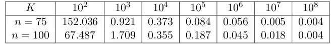
K 102 103 104 105 106 107 108 n= 75 152.036 0.921 0.373 0.084 0.056 0.005 0.004
n= 100 67.487 1.709 0.355 0.187 0.045 0.018 0.004
Table 1: Approximation of the partition function via the IS for the footrule model:
maxi-mum relative error K from equation (10), between the current and the previous
K, forn= 75 and 100.
When nis larger than 50,no exact expression for Zn(α) is available. Then, we directly
compare the estimated ˆZnK(α) for increasing K, to check whether the estimates stabilize.
We thus inspect the maximum relative error
K = max
α
ˆ
ZK
n (α)−Zˆ K/10
n (α)
ˆ
ZnK/10(α)
(10)
forK = 102, . . . ,108. Results are shown in Table 1 for n= 75 and 100. For both values of
n we see that the estimates quickly stabilize, and K = 106 appears to give good
approx-imations. The computations shown here were performed on a desktop computer, and the
off-line computation with K = 106 samples for n= 10 took less than 15 minutes, with no
efforts for parallelizing the algorithm, which would be easy and beneficial. K= 106samples
forn= 100 were obtained on a 64-cores computing cluster in 12 minutes.
3.2 Effect of Zˆn(α) on the MCMC
Proposition 2 Algorithm 1 of Appendix B using Zˆn(α) in (9) instead of Zn(α) converges to the posterior distribution proportional to
1 ˆ
C(R)π(ρ)π(α) ˆZn(α)
−Nexp
−α
n
N X
j=1
d(Rj,ρ)
, (11)
with the normalizing factor Cˆ(R) =R ˆπ(α)
Zn(α)N
P
ρ∈Pnπ(ρ) exp
n
−αnPN
j=1d(Rj,ρ) o
dα.
Proof The acceptance probability of the MCMC in Algorithm 1 with the approximate
partition function is given by (8) using ˆZn(α) in (9) instead of Zn(α), which is exactly the
acceptance probability needed for (11).
That ˆC(R)<∞is an obvious consequence of our assumption, in Section 2.2, that the prior
π(α) is supported by a finite interval [0, αmax]. The IS approximation ˆZn(α) converges to
Zn(α) as the number K of IS samples converges to infinity. In order to study this limit,
let us change the notation to explicitly show this dependence and write ˆZnK(α). Clearly,
the approximate posterior (11) converges to the correct posterior (4) ifK increases withN,
K =K(N),and
lim
N→∞
ˆ
ZnK(N)(α)
Zn(α)
!N
= 1, for all α. (12)
Proposition 3 There exists a factor c(α, n, d(·,·)) not depending on N, such that, if K=
K(N) tends to infinity asN → ∞ faster than c(α, n, d(·,·))·N2, then (12) holds.
Proof We see that
ˆ
ZnK(N)(α)
Zn(α)
!N
= exp (
Nlog 1 +Zˆ
K(N)
n (α)−Zn(α)
Zn(α)
!)
tends to 1 in probability asK(N)→ ∞when N → ∞ if
ˆ
ZnK(N)(α)−Zn(α)
Zn(α)
(13)
tends to 0 in probability faster than 1/N. Since (9) is a sum of i.i.d. variables, there exists
a constantc=c(α, n, d(·,·)) depending onα, nand the distanced(·,·) (but not onN) such
that
p
K(N)( ˆZnK(N)(α)−Zn(α))
L
→ N(0, c2),
in law as K(N) → ∞. Therefore, for (13) tending to 0 faster than 1/N, it is sufficient
that K(N) grows faster than N2. The speed of convergence to 1 of (12) depends on
0.0 0.5 1.0 1.5 2.0 2.5 3.0
0
1
2
3
4
5
6
7
Exact partition function
α
density
N = 20 N = 50 N = 100
unif prior exp(0.1) prior exp(1) prior exp(10) prior
0.0 0.5 1.0 1.5 2.0 2.5 3.0
0
1
2
3
4
5
6
7
IS approximated partition function, K large
α
density
N = 20 N = 50 N = 100
unif prior exp(0.1) prior exp(1) prior exp(10) prior
0.0 0.5 1.0 1.5 2.0 2.5 3.0
0
1
2
3
4
5
6
7
IS approximated partition function, K small
α
density
N = 20 N = 50 N = 100
unif prior exp(0.1) prior exp(1) prior exp(10) prior
1 2 3 4 5
0
1
2
3
4
5
6
7
Exact partition function
α
density
N = 20 N = 50 N = 100
unif prior exp(0.1) prior exp(1) prior exp(10) prior
1 2 3 4 5
0
1
2
3
4
5
6
7
IS approximated partition function, K large
α
density
N = 20 N = 50 N = 100
unif prior exp(0.1) prior exp(1) prior exp(10) prior
1 2 3 4 5
0
1
2
3
4
5
6
7
IS approximated partition function, K small
α
density
N = 20 N = 50 N = 100
unif prior exp(0.1) prior exp(1) prior exp(10) prior
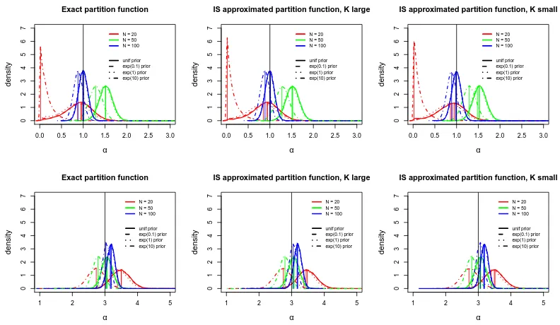
Figure 2: Results of the simulations described in Section 3.3, when n = 20. In each plot,
posterior density ofα(the black vertical line indicatesαtrue) obtained for various
choices ofN (different colors), and for different choices of the prior forα(different
line types), as stated in the legend. From left to right, MCMC run with the
exactZn(α), with the IS approximation ˆZnK(α) with K = 108, and with the IS
approximation ˆZnK(α) withK = 104. First row: αtrue= 1; second row: αtrue= 3.
3.3 Testing Approximations of the MCMC in Inference
We report results from extensive simulation experiments carried out in several different parameter settings, to investigate if our algorithm provides correct posterior inferences. In addition, we study the sensitivity of the posterior distributions to differences in the prior
specifications, and demonstrate their increased precision when the sample size N grows.
We explore the robustness of inference when using approximations of the partition function
Zn(α), both when obtained by applying our IS approach, and when using, for largen, the
asymptotic approximation Zlim(α) proposed in Mukherjee (2016). We focus here on the
footrule distance since it allows us to explore all these different settings, being also the preferred distance in the experiments reported in Section 6. Some model parameters are
kept fixed in the various cases: αjump= 10, σα = 0.15,and L=n/5 (for the tuning of the
two latter parameters, see the simulation study in the Supplementary Material, Section 1). Computing times for the simulations, performed on a laptop computer, varied depending
on the value of n and N, from a minimum of 2400 in the smallest case with n = 20 and
N = 20,to a maximum of 302200 forn= 100 andN = 1000.
First, we generated data from a Mallows model with n= 20 items, using samples from
0 2 4 6 8 10 0.0 0.2 0.4 0.6 0.8 1.0
Exact partition function
d(ρ, ρtrue)
CDF ●● ●●●●●●●●●●●● ●●●●● ● ●● ● ● ● ● ● ● ● ● ● ● ●● ●● ●●●●●●● ●●●●●●●●●●●●●●●●● ●●●●●● ● ● ●●●●●●●●●●●●●● ●●● ●● ● ● ● ● ● ● ● ● ● ● ● ●● ●● ●● ●● ●●●●●●●●●●●●●●●●●●● ●●●● ● ● ●●●●●●●●●●●●●● ●●●●● ●● ● ●● ● ● ● ● ● ● ● ● ●● ●● ●● ●●●● ●●●●●●● ●●●●●●●●●●●●●●●●● ●● ● ●● ● ●●●●●●●●●●●●●●●●●●● ●●●● ●● ●● ● ●● ●● ● ●● ●● ●● ●●● ●● ●●●●● ●●●●●●●●●●●●●●● ●●●●●●● ● ● ● ● ● ● ● ● ● ● ● ●● ●●●●●●● ● ● ●●●●●●● ● ● ● ● ● ● ● ● ● ● ● ● ●● ●●●●●●●●● ● ●●●●●●●● ● ● ● ● ● ● ● ● ● ● ● ●● ●●●●●●●●●● ● ●●●●●●●● ● ● ● ● ● ● ● ● ● ● ● ●● ●●●●●●●●●●●● ● ●●●●●●●●●●● ● ● ● ● ● ● ● ● ● ● ● ●●●●●●●●●●● ●● ●●●●●●●●●● ● ● ● ● ● ● ● ● ● ● ●● ●●●●●●●●●●●● ● ●●●●●●●● ● ● ● ● ● ● ● ● ● ● ● ● ● ●●●●●●●●●●● ● ●●●●●●●● ● ● ● ● ● ● ● ● ● ● ● ●● ●●●●●●●●●●● ●
N = 20 N = 50 N = 100
unif prior exp(0.1) prior exp(1) prior exp(10) prior
0 2 4 6 8 10
0.0 0.2 0.4 0.6 0.8 1.0
IS approximated partition function, K large
d(ρ, ρtrue)
CDF ●●●●●●●●●●●●●●●● ●●●● ●● ● ● ● ● ● ● ● ● ● ● ●● ● ●●● ●●●●● ●●●●●●●●●●●●● ●●●●●●●● ● ●●●●●●●●●●●●● ●●●● ●● ● ● ● ● ● ● ● ● ● ● ● ●● ●● ●●●●●●●●●●●● ●●●●●●●●●●●●●●●● ● ●●●●●●●●●●●●●●●●●● ●● ● ● ● ● ● ● ● ● ● ● ●● ●● ●● ●●●●●● ●●●●●●●●●●●●●●●●●●●●●●● ● ●●●●●●●●●●●●●●●●●●●●●● ●●● ●●● ● ●● ● ●● ● ●● ● ●● ●● ●● ●●●●●●●● ●●●●●●●●●●●●●●●●● ● ●●●●●●●● ● ● ● ● ● ● ● ● ● ● ● ● ● ●●●●●●●●●●● ●●●●●●●●● ● ● ● ● ● ● ● ● ● ● ● ●● ●●●●●●●● ● ●●●●●●● ●● ● ● ● ● ● ● ● ● ● ● ●● ●●●●●●●●●● ●● ●●●●●●●●● ● ● ● ● ● ● ● ● ● ● ●● ●●●●●●●●●● ●●●●●●● ● ● ● ● ● ● ● ● ● ● ● ●● ●●●●●●●●●●● ● ●●●●●●●● ● ● ● ● ● ● ● ● ● ● ● ●● ●●●●●●●●●●● ●●●●●●●●● ● ● ● ● ● ● ● ● ● ● ●● ●●●●●●●●●●● ● ●●●●●●●●● ● ● ● ● ● ● ● ● ● ● ● ●● ●●●●●●●●●●●
N = 20 N = 50 N = 100
unif prior exp(0.1) prior exp(1) prior exp(10) prior
0 2 4 6 8 10
0.0 0.2 0.4 0.6 0.8 1.0
IS approximated partition function, K small
d(ρ, ρtrue)
CDF ●●● ●●●●●●●●●●●● ●●● ●● ● ● ● ● ● ● ● ● ● ● ● ●● ●● ●●● ●●●●● ●●●●●●●●●●●●●●●●●●●●●● ● ●●●●●●●●●●●●●●● ●●●● ●● ● ● ● ● ● ● ● ● ● ● ● ● ●● ●● ●● ●●●●●●●●●●●●●●●●●●●●●●●●●● ● ●●●●●●●●●●●●●●●● ●● ● ● ● ● ● ● ● ● ● ● ●● ● ●● ●● ●●●●● ●●●●●●●●●●●●●●●●●●●● ● ● ●●●●●●●●●●●●●●●●●●●●●●●● ●●●●● ●● ●● ●● ● ● ● ●● ●● ●● ●● ●● ●●●●●● ●●●●●●●●●●●●●●●● ● ● ●●●●●●●● ● ● ● ● ● ● ● ● ● ● ● ●● ●●●●●●●●●●●● ●●●●●●● ● ● ● ● ● ● ● ● ● ● ● ●● ●●●●●●●●●●●● ● ● ●●●●●●● ● ● ● ● ● ● ● ● ● ● ● ● ●● ●●●●●●●● ● ● ●●●●●●●● ● ● ● ● ● ● ● ● ● ● ● ● ● ● ●●●●●●●●●● ●●●●●●●●● ● ● ● ● ● ● ● ● ● ● ● ●● ●●●●●●●●●●● ●●●●●●● ● ● ● ● ● ● ● ● ● ● ● ●● ●●●●●●●●●● ●●●●●●●●● ● ● ● ● ● ● ● ● ● ● ● ● ●●●●●●●●●●●● ● ●●●●●●●● ● ● ● ● ● ● ● ● ● ● ● ● ●● ●●●●●●●●●●● ●
N = 20 N = 50 N = 100
unif prior exp(0.1) prior exp(1) prior exp(10) prior
0 2 4 6 8 10
0.0 0.2 0.4 0.6 0.8 1.0
Exact partition function
d(ρ, ρtrue)
CDF ●●●●●●● ● ● ● ● ● ● ● ● ● ●●●●●●●●●● ● ●●●●●● ● ● ● ● ● ● ● ● ● ●●● ●●●●●● ● ●●●●●● ● ● ● ● ● ● ● ● ● ●● ●●●●●●●● ● ●●●●●●● ● ● ● ● ● ● ● ● ● ● ●●●●●●●●● ● ●●●● ● ● ● ● ● ● ● ●●●●●●● ● ●●●● ● ● ● ● ● ● ● ●●●●●● ● ●●●● ● ● ● ● ● ● ● ●●●●●● ● ● ●●● ● ● ● ● ● ● ● ● ●●●●●● ● ● ● ● ● ● ● ● ●●● ● ● ●● ● ● ● ● ● ●●●● ● ● ● ● ● ● ● ● ● ●●● ● ● ●● ● ● ● ● ● ●●●● ● ● ●
N = 20 N = 50 N = 100
unif prior exp(0.1) prior exp(1) prior exp(10) prior
0 2 4 6 8 10
0.0 0.2 0.4 0.6 0.8 1.0
IS approximated partition function, K large
d(ρ, ρtrue)
CDF ●●●●●● ● ● ● ● ● ● ● ● ● ●●● ●●●●● ● ● ● ●●●●● ● ● ● ● ● ● ● ● ● ● ●●●●●●●● ● ●●●●●●● ● ● ● ● ● ● ● ● ● ●●●●●●●●● ● ●●●●●●● ● ● ● ● ● ● ● ● ● ●● ●●●●●●●● ● ●●● ● ● ● ● ● ● ● ●●●●●●● ● ●●● ● ● ● ● ● ● ● ●●●●● ● ● ●●●● ● ● ● ● ● ● ● ●●●●●● ● ● ●●●● ● ● ● ● ● ● ● ●●●●●●● ● ● ● ● ● ● ● ● ●●●● ● ● ● ● ● ● ● ● ● ●●●● ● ●● ● ● ● ● ● ●●●●● ● ●● ● ● ● ● ● ●●●● ● ● ●
N = 20 N = 50 N = 100
unif prior exp(0.1) prior exp(1) prior exp(10) prior
0 2 4 6 8 10
0.0 0.2 0.4 0.6 0.8 1.0
IS approximated partition function, K small
d(ρ, ρtrue)
CDF ● ●●●●●● ● ● ● ● ● ● ● ● ● ● ●●●●●●●●●●● ● ●●●●●●● ● ● ● ● ● ● ● ● ● ● ●●●●●●● ●● ● ● ● ●●●●● ● ● ● ● ● ● ● ● ● ●● ●●●●●●● ● ●●●●●●● ● ● ● ● ● ● ● ● ● ● ●●●●●●●● ●●● ● ● ● ● ● ● ● ●●●●●●●● ●●●● ● ● ● ● ● ● ● ●●●●●●● ●●●● ● ● ● ● ● ● ● ●●●●●● ● ●●●● ● ● ● ● ● ● ● ●●● ●●● ● ● ●● ● ● ● ● ● ●●●● ● ● ● ● ● ● ● ● ● ●●●● ● ●● ● ● ● ● ● ●●●● ● ● ●● ● ● ● ● ● ●●●● ● ●
N = 20 N = 50 N = 100
unif prior exp(0.1) prior exp(1) prior exp(10) prior
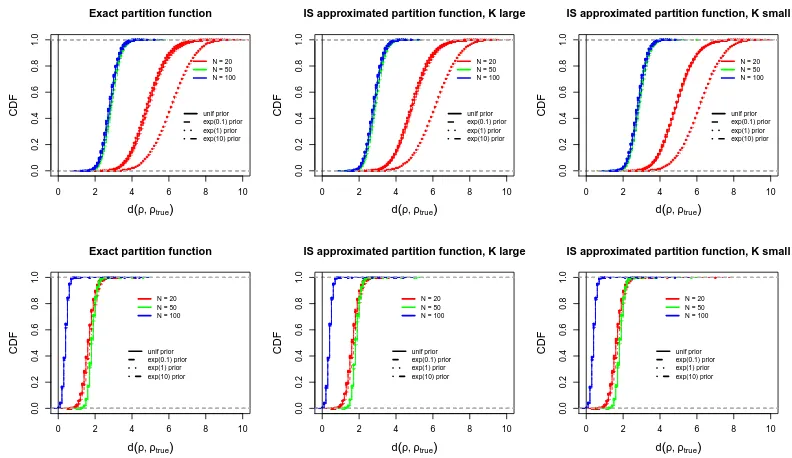
Figure 3: Results of the simulations described in Section 3.3, when n = 20. In each plot,
posterior CDF of d(ρ,ρtrue) obtained for various choices of N (different colors),
and for different choices of the prior for α (different line types), as stated in
the legend. From left to right, MCMC run with the exact Zn(α), with the IS
approximation ˆZnK(α) withK = 108, and with the IS approximation ˆZnK(α) with
K= 104. First row: αtrue= 1; second row: αtrue= 3.
chosen to be either 1 or 3, and ρtrue was fixed at (1, . . . , n). To generate the data, we run
the MCMC sampler (see Appendix C) for 105 burn-in iterations, and collected one sample
every 100 iterations after that (these settings were kept in all data generations). In the analysis, we considered the performance of the method when using the IS approximation
ˆ
ZnK(α) with K = 104 and 108, then comparing the results with those based on the exact
Zn(α). In each case, we run the MCMC for 106 iterations, with 105 iterations for burn-in.
Finally, we varied the prior forα to be either the nonintegrable uniform or the exponential
using hyperparameter values λ = 0.1,1 and 10. The results are shown in Figures 2 for
α and 3 for ρ. As expected, we can see the precision and the accuracy of the marginal
posterior distributions increasing, both for α and ρ, with N becoming larger. For smaller
values ofαtrue,the marginal posterior forαis more dispersed, andρis stochastically farther
from ρtrue.These results are remarkably stable against varying choices of the prior for α,
even when the quite strong exponential prior with λ = 10 was used (with one exception:
in the case of N = 20 the rather dispersed data generated by αtrue = 1 were not sufficient
to overcome the control of the exponential prior with λ= 10, which favored even smaller
values of α; see Figure 2, top panels). Finally and most importantly, we see that inference
on both α and ρ is completely unaffected by the approximation of Zn(α) already when
0.0 0.5 1.0 1.5 2.0 2.5 3.0
0
5
10
15
Posterior density of alpha
α
density
N = 50 N = 500
Z exact Z approx IS, K large Z approx IS, K small Z asymptotics
0 5 10 15 20
0.0 0.2 0.4 0.6 0.8 1.0
PosteriorCDFof d(ρ, ρtrue)
d(ρ, ρtrue)
CDF ●●●●●●●●●●●●●●●●●●●●●●●●●●●●●●●●●●● ● ●●●● ● ●● ● ●● ●● ● ●● ●● ● ●● ●●●●●●●●●●●●●●●●●●●●●●●●●●●●●●●●●●●●●● ● ●●●●●●●●●●●●●●●●●●●●●● ●● ● ●● ●● ● ● ● ●● ● ●● ●● ● ●●●●●●●●●●●●●●●●●●●●●● ● ● ● ● ●●●●●●●●●●●●●●●●●●●●●●●●●●●●●●●● ●●●● ● ●● ● ●● ●● ● ●●● ●● ●● ●● ● ●●●●●●●●●●●●●●●●●●●●●●●●●●●●●●●●●●●●●●●●● ● ●●● ● ● ●●●●●●●●●●●●●●●●●●●●●● ●● ● ●● ●● ● ●● ● ●● ●● ●● ● ●●●●●●●●●●●●●●●●●●●●●●● ● ● ● ●●●●●●●●●●●●●●●●●●●●●●●●●●●●●●●●●●●●●●● ●●● ●● ●● ● ●● ●● ● ●● ●● ● ●●●●●●●●●●●●●●●●●●●●●●●●●●●●●●●●●●●●●●●●● ● ● ● ●●●●●●●●●●●●●●●●●●●●● ● ●● ● ●● ● ●● ●● ●● ● ●● ●● ● ●●●●●●●●●●●●●●●●●●●●●●● ● ● ● ●●●●●●●●●●●●●●●●●●●●●●●●●●●●●●●●●●● ●● ●● ●● ● ●● ●● ● ●● ●● ● ●● ●●● ●●●●●●●●●●●●●●●●●●●●●●●●●●●●●●●●●●●●● ●●●●●●●●●●●●●●●●●●●●●● ● ●● ● ● ● ● ●● ●● ●● ● ●● ●● ● ●●● ●●●●●●●●●●●●●●●●●●●● ● ● ● ●
N = 50 N = 500
Z exact Z approx IS, K large Z approx IS, K small Z asymptotics
3 4 5 6 7
0 2 4 6 8 10
Posterior density of alpha
α
density
N = 50 N = 500
Z exact Z approx IS, K large Z approx IS, K small Z asymptotics
0 2 4 6 8 10
0.0 0.2 0.4 0.6 0.8 1.0
PosteriorCDFof d(ρ, ρtrue)
d(ρ, ρtrue)
CDF ●●●●●●●●●●●● ● ● ● ● ● ● ● ● ● ● ●● ●● ●●●●●●●●●●●●●● ● ● ● ●●● ● ● ● ● ● ● ●●●●● ●●● ● ● ● ● ● ● ●●●●●●●●●●●● ● ● ● ● ● ● ● ● ● ● ● ●● ●●●●●●● ●●●●●● ● ● ● ● ● ●●● ● ● ● ● ● ● ●●●●● ● ● ● ● ● ● ● ● ●●●●●●●●●● ●● ● ● ● ● ● ● ● ● ● ● ●● ●●●●●●●●●●●●● ●● ●● ● ● ● ●●● ● ● ● ● ● ● ●●●●●● ●● ● ● ● ● ● ● ● ●●●●●●●●●●●● ● ● ● ● ● ● ● ● ● ● ●● ●●●●●●●●●●●●● ●●● ● ● ●● ● ●●● ● ● ● ● ● ● ●●●●● ●● ●●● ● ● ● ● ●
N = 50 N = 500
Z exact Z approx IS, K large Z approx IS, K small Z asymptotics
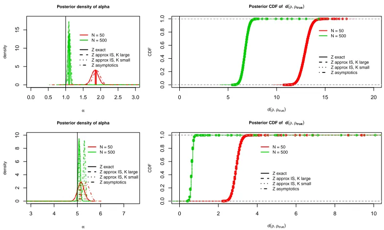
Figure 4: Results of the simulations described in Section 3.3, when n= 50. Left, posterior
density of α (the black vertical line indicates αtrue) obtained for various choices
of N (different colors), and when using the exact, or different approximations
to the partition function (different line types), as stated in the legend. Right,
posterior CDF of d(ρ,ρtrue) in the same settings. First row: αtrue = 1; second
row: αtrue= 5.
In a second experiment, we generated data using n= 50 items,N = 50 or 500 assessors,
and scale parameterαtrue= 1 or 5. This increase in the value of n gave us some basis for
comparing the results obtained by using the IS approximation of Zn(α) with those from
the asymptotic approximation Zlim(α) of Mukherjee (2016), while still retaining also the
possibility of using the exactZn(α). For the analysis, all the previous MCMC settings were
kept, except for the prior forα: since results fromn= 20 turned out to be independent of the
choice of the prior, here we used the same exponential prior withλ= 0.1 in all comparisons
(see the discussion in Section 2.2). The results are shown in Figures 4 and 5. Again, we
observe substantially more accurate results for larger values of N and αtrue. Concerning
the impact of approximations to Zn(α), we notice that, even in this case of larger n, the
marginal posterior of ρ appears completely unaffected by the partition function not being
exact (see Figure 4, right panels, and Figure 5). In the marginal posterior forα (Figure 4,
left panels), there are no differences between using the IS approximations and the exact,
but there is a difference between Zlim and the other approximations: Zlim appears to be
systematically slightly worse.
Finally, we generated data from the Mallows model with n = 100 items, N = 100 or
1000 assessors, and using αtrue = 5 or 10. Because of this large value of n we were no
10 20 30 40 50
10
20
30
40
50
Exact
0.0 0.1 0.2 0.3 0.4 0.5
10 20 30 40 50
10
20
30
40
50
IS K=108
0.0 0.1 0.2 0.3 0.4 0.5
10 20 30 40 50
10
20
30
40
50
IS K=104
0.0 0.1 0.2 0.3 0.4 0.5
10 20 30 40 50
10
20
30
40
50
Asymptotics
0.0 0.1 0.2 0.3 0.4 0.5
10 20 30 40 50
10
20
30
40
50
Exact
0.0 0.2 0.4 0.6 0.8
10 20 30 40 50
10
20
30
40
50
IS K=108
0.0 0.2 0.4 0.6 0.8
10 20 30 40 50
10
20
30
40
50
IS K=104
0.0 0.2 0.4 0.6 0.8
10 20 30 40 50
10
20
30
40
50
Asymptotics
0.0 0.2 0.4 0.6 0.8
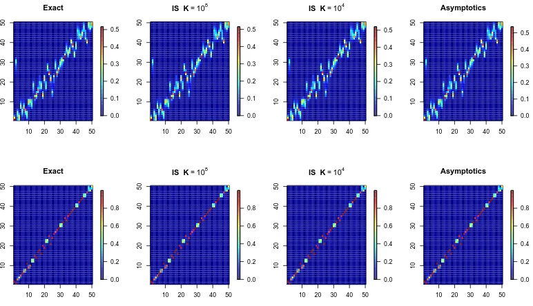
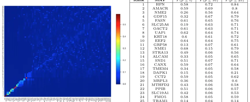
Figure 5: Results of the simulations described in Section 3.3, when n = 50 and αtrue =
5. In the x-axis items are ordered according to the true consensus ρtrue. Each
columnj represents the posterior marginal density of itemj in the consensusρ.
Concentration along the diagonal is a sign of success of inference. From left to
right, results obtained with the exact Zn(α), with the IS approximation ˆZnK(α)
withK = 108, with the IS approximation ˆZnK(α) withK = 104,and withZlim(α).
First row: N = 50; second row: N = 500.
approximations. We kept the same MCMC settings as forn= 50, both in data generation
and analysis. The results are shown in Figures 3 and 4 of the Supplementary Material, Section 3. Also in this case, we observe substantially more accurate estimates with larger
values of N and αtrue, establishing an overall stable performance of the method. Here,
using the small number K = 104 of samples in the IS approximation has virtually no
effect on the accuracy of the marginal posterior for α, while a small effect can be detected
from using the asymptotic approximation (Figure 3 of the Supplementary Material, left
panels). However, again, the marginal posterior forρappears completely unaffected by the
considered approximations in the partition function (Figure 3, right panels, and Figure 4 of the Supplementary Material).
In conclusion, the main positive result from the perspective of practical applications was the relative lack of sensitivity of the posterior inferences to the specification of the prior for
the scale parameterα, and the apparent robustness of the marginal posterior inferences on
ρon the choice of the approximation of the partition function Zn(α). The former property
The second observation deserves a somewhat closer inspection, however. The
margi-nal posterior P(α|R), considered in Figures 2 and 4 (left), and in Figure 3 (left) of the
Supplementary Material, is obtained from the joint posterior (4) by simple summation over
ρ,then getting the expression
P(α|R)∝π(α)C(α;R)/(Zn(α))N, (14)
whereC(α;R) =P
ρ∈Pnπ(ρ) exp
n −α
n
PN
j=1d(Rj,ρ) o
. For a proper understanding of the
structure of the joint posterior and its modification (11), it is helpful to first factorize (4) into the product
P(α,ρ|R) =P(α|R)P(ρ|α,R), (15) where then
P(ρ|α,R) = [C(α;R)]−1π(ρ) exp
−α
n
N X
j=1
d(Rj,ρ)
. (16)
The joint posterior (11), which arises from replacing the partition function Zn(α) by its
approximation ˆZn(α), can be similarly expressed as the product
ˆ
P(α,ρ|R) = ˆP(α|R)P(ρ|α,R), (17)
where
ˆ
P(α|R) = [ ˆC(R)]−1(Zn(α)/Zˆn(α))NP(α|R). (18)
This requires that the normalizing factor ˆC(R) already introduced in (11), and here
ex-pressed as
ˆ
C(R)≡ Z
(Zn(α)/Zˆn(α))NP(α|R)dα, (19)
is finite. By comparing (15) and (17) we see that, under this condition, the posterior
ˆ
P(α,ρ|R) arises fromP(α,ρ|R) by changing the expression (14) of the marginal posterior
forα into (18), while the conditional posterior P(ρ|α,R) for ρ, given α,remains the same
in both cases. Thus, the marginal posteriorsP(ρ|R) and ˆP(ρ|R) forρarise as mixtures of
the same conditional posteriorP(ρ|α,R) with respect to two different mixing distributions,
P(α|R) and ˆP(α|R).
It is obvious from (18) and (19) that ˆP(α|R) =P(α|R) would hold if the ratioZn(α)/
ˆ
Zn(α) would be exactly a constant in α, and this would also entail the exact equality
ˆ
P(ρ|R) =P(ρ|R). It was established in (12) that, in the IS scheme, Zn(α)/Zˆn(α)→ 1 as
K → ∞. Thus, for large enough K, (Zn(α)/Zˆn(α))N ≈1 holds as an approximation (see
Proposition 3). Importantly, however, (18) shows that the approximation is only required
to hold well on the effective support ofP(α|R), and this support is narrow whenN is large.
This is demonstrated clearly in Figures 2 and 4 (left), and in Figure 3 (left) of the
Supple-mentary Material. On this support, because of uniform continuity in α, also the integrand
P(ρ|α,R) in (16) remains nearly a constant. In fact, experiments (results not shown)
per-formed by varying α over a much wider range of fixed values, while keeping the same R,
gave remarkably stable results for the conditional posteriorP(ρ|α,R). This contributes to
the high degree of robustness in the posterior inferences onρ, making requirements of using
In Figures 3 and 4 (right), and in Figure 3 (right) of the Supplementary Material, we
considered and compared the marginal posterior CDF’s of the distance d(ρ,ρtrue) under
the schemes P(·|R) and ˆP(·|R). Using the shorthand d∗ =d(ρ,ρtrue), let
Fd∗(x|α,R) ≡ P(d(ρ,ρtrue)≤x|α,R) =
X
{ρ:d(ρ,ρtrue)≤x}
P(ρ|α,R), (20)
Fd∗(x|R) ≡
X
{ρ:d(ρ,ρtrue)≤x}
P(ρ|R) = Z
Fd∗(x|α,R)P(α|R)dα,
ˆ
Fd∗(x|R) ≡
X
{ρ:d(ρ,ρtrue)≤x} ˆ
P(ρ|R) = Z
Fd∗(x|α,R) ˆP(α|R)dα.
For example, in Figure 3 we display, for different priors, the CDF’sFd∗(x|R) on the left, and
ˆ
Fd∗(x|R) in the middle and on the right, corresponding to two different IS approximations
of the partition function. Like the marginal posteriorsP(ρ|R) and ˆP(ρ|R) above,Fd∗(x|R)
and ˆFd∗(x|R) can be thought of as mixtures of the same function, hereFd∗(x|α,R), but with
respect to two different mixing distributions, P(α|R) and ˆP(α|R). The same arguments,
which were used above in support of the robustness of the posterior inferences onρ, apply
here as well. Extensive empirical evidence for their justification is provided in Figures 3 and 4 (right), and in Figure 3 (right) of the Supplementary Material. Finally note that these arguments also strengthen considerably our earlier conclusion of the lack of sensitivity of
the posterior inferences onρto the specification of the prior forα. For this, we only need to
consider alternative priors, say,π(α) and ˆπ(α), in place of the mixing distributionsP(α|R)
and ˆP(α|R).
4. Extensions to Partial Rankings and Heterogeneous Assessor Pool
We now relax two assumptions of the previous Sections, namely that each assessor ranks all
nitems and that the assessors are homogeneous, all sharing a common consensus ranking.
This allows us to treat the important situation of pairwise comparisons, and of multiple classes of assessors, as incomplete data cases, within the same Bayesian Mallows framework.
4.1 Ranking of the Top Ranked Items
Often only a subset of the items is ranked: ranks can be missing at random, the assessors
may only have ranked the, in-their-opinion, top-kitems, or can be presented with a subset of
items that they have to rank. These situations can be handled conveniently in our Bayesian framework, by applying data augmentation techniques. We start by explaining the method
in the case of the top-kranks, and then show briefly how it can be generalized to the other
cases mentioned.
Suppose that each assessor j has ranked the subset of items Aj ⊆ {A1, A2, . . . , An},
giving them top ranks from 1 tonj =|Aj|. LetRij =X−j1(Ai) ifAi ∈ Aj, while forAi∈ Acj,
Rij is unknown, except for the constraint Rij > nj,j = 1, . . . , N, and follows a symmetric
prior on the permutations of (nj+ 1, . . . , n). We define augmented data vectors ˜R1, . . . ,R˜N
by assigning ranks to these non-ranked items randomly, using an MCMC algorithm, and
X−j1(Ai) if Ai ∈ Aj}, j = 1, . . . , N, be the set of possible augmented random vectors, that
is the original partially ranked items together with the allowable “fill-ins” of the missing ranks. Our goal is to sample from the posterior distribution
P(α,ρ|R1, . . . ,RN) = X
˜
R1∈S1
· · · X
˜
RN∈SN
Pα,ρ,R˜1, . . . ,R˜N|R1, . . . ,RN
.
Our MCMC algorithm alternates between sampling the augmented ranks given the current
values ofα and ρ,and sampling α andρ given the current values of the augmented ranks.
For the latter, we sample from the posteriorP(α,ρ|R1, . . . ,˜ R˜N) as in Section 2.4. For the
former, fixing α and ρ and the observed ranks R1, . . . ,RN, we see that ˜R1, . . . ,R˜N are
conditionally independent, and moreover, that each ˜Rj only depends on the corresponding
Rj. This enables us to consider the sampling of new augmented vectors ˜R0j separately
for each j, j = 1, . . . , N. Specifically, given the current ˜Rj (which embeds information
contained in Rj) and the current values for α and ρ, ˜R0j is sampled inSj from a uniform
proposal distribution, meaning that the highest ranks from 1 to nj have been reserved for
the items inAj, while compatible ranks are randomly drawn for items inAc
j. The proposed
˜
R0j is then accepted with probability
min n
1,exp
h −α
n
d( ˜R0j, ρ)−d( ˜Rj, ρ) io
. (21)
The MCMC algorithm described above and used in the case of partial rankings is given in Algorithm 3 of Appendix B. Our algorithm can also handle situations of generic partial
ranking, where each assessor is asked to provide the mutual ranking of some subset Aj ⊂
{A1, ..., An}consisting ofnj ≤nitems, not necessarily the top-nj. In this case, we can only
say that in ˜Rj = ( ˜R1j, ...,R˜nj) the order between items Ai ∈ Aj must be preserved as in
Rj, whereas the ranks of the augmented “fill-ins”Ai ∈ Acj are left open. More exactly, the
latent rank vector ˜Rj takes values in the setSj ={R˜j ∈ Pn: ifRi1j < Ri2j, withAi1, Ai2 ∈
Aj ⇒R˜i1j <R˜i2j}. The MCMC is then easily adjusted so that the sampling of each ˜Rj is
restricted to the correspondingSj, thus respecting the mutual rank orderings in the data.
4.1.1 Effects of Unranked Items on the top-k Consensus Ranking
In applications in which the number of items is large there are often items which none of the assessors included in their top-list. What is the exact role of such “left-over” items in
the top-kconsensus ranking of all items? Can we ignore such “left-over” items and consider
only the items explicitly ranked by at least one assessor? In the following we first show that only items explicitly ranked by the assessors appear in top positions of the consensus ranking. We then show that, when considering the MAP consensus ranking, excluding the left-over items from the ranking procedure already at the start has no effect on how the remaining ones will appear in such consensus ranking.
For a precise statement of these results, we need some new notation. Suppose that
assessor j has ranked a subset Aj of nj items. Let A=Sj=1,...,NAj, and denote n=|A|.
Letn∗ be the total number of items, including left-over items which have not been explicitly
ranked by any assessor. Denote by A∗ ={Ai;i= 1, . . . , n∗}the collection of all items, and
by Ac =A∗\ A the left-over items. Each rank vector R
order, the ranks from 1 to nj given to items in Aj. In the original data the ranks of all
remaining items are left unspecified, apart from the fact that implicitly, for assessorj, they
would have values which are at least as large as nj+ 1.
The results below are formulated in terms of the two different modes of analysis, which we need to compare and which correspond to different numbers of items being included.
The first alternative is to include in the analysis the complete set A∗ of n∗ items, and
to complement each data vector Rj by assigning (originally missing) ranks to all items
which are not included in Aj; their ranks will then form some permutation of the sequence
(nj + 1, . . . , n∗). We call this mode of analysisfull analysis, and denote the corresponding
probability measure by Pn∗. The second alternative is to include in the analysis only the
items which have been explicitly ranked by at least one assessor, that is, items belonging
to the set A. We call this second mode restricted analysis, and denote the corresponding
probability measure byPn. The probability measurePnis specified as before, including the
uniform prior on the consensus ranking ρ across all n! permutations of (1,2, . . . , n), and
the uniform prior of the unspecified ranks Rij of items Ai ∈ Acj across the permutations
of (nj + 1, . . . , n). The definition of Pn∗ is similar, except that then the uniform prior
distributions are assumed to hold in the complete setA∗of items, that is, over permutations
of (1,2, . . . , n∗) and (nj+ 1, . . . , n∗), respectively. In the posterior inference carried out in
both modes of analysis, the augmented ranks, which were not recorded in the original data, are treated as random variables, with values being updated as part of the MCMC sampling.
Proposition 4 Consider two latent consensus rank vectors ρ and ρ0 such that
(i) in the ranking ρ all items in A have been included among the top-n-ranked, while
those in Ac have been assigned ranks between n+ 1 and n∗,
(ii) ρ0 is obtained from ρ by a permutation, where the rank in ρ of at least one item
belonging to A has been transposed with the rank of an item in Ac.
Then, Pn∗(ρ|data)≥Pn∗(ρ0|data), for the footrule, Kendall and Spearman distances in the
full analysis mode.
Remark. The above proposition says, in essence, that any consensus lists of top-nranked items, which contains one or more items with their ranks completely missing in the data (that is, the item was not explicitly ranked by any of the assessors), can be improved
locally, in the sense of increasing the associated posterior probability with respect to Pn∗.
This happens by trading such an item in the top-n list against another, which had been
ranked but which had not yet been selected to the list. In particular, the MAP estimate(s)
for consensus ranking assign nhighest ranks to explicitly ranked items in the data (which
corresponds to the result in Meilˇa and Bao (2010) for Kendall distance). The following
statement is an immediate implication of Proposition 4, following from a marginalization
with respect toPn∗.
Corollary 1 Consider, for k≤n, collections {Ai1, Ai2, . . . , Aik} of k items and the
corre-sponding ranks {ρi1, ρi2, . . . , ρik}. In full analysis mode, the maximal posterior probability
Pn∗({ρi
Another consequence of Proposition 4 is the coincidence of the MAP estimates under the
two probability measures Pn and Pn∗.
Corollary 2 Denote by ρM AP∗ the MAP estimate for consensus ranking obtained in a full
analysis, ρM AP∗ := argmaxρ∈Pn∗Pn∗(ρ|data), and by ρ
M AP the MAP estimate for
con-sensus ranking obtained in a restricted analysis, ρM AP := argmaxρ∈PnPn(ρ|data). Then,
ρM AP∗|i:Ai∈A≡ρ
M AP.
Remark. The above result is very useful in the context of applications, since it guarantees
that the top-nitems in the MAP consensus ranking do not depend on which version of the
analysis is performed. Recall that a full analysis cannot always be carried out in practice, due to the fact that left-over items might be unknown, or their number might be too large for any realistic computation.
4.2 Pairwise Comparisons
In many situations, assessors compare pairs of items rather than ranking all or a subset of items. We extend our Bayesian data augmentation scheme to handle such data. Our approach is an alternative to Lu and Boutilier (2014), who treated preferences by applying their Repeated Insertions Model (RIM). Our approach is simpler, it is fully integrated into our Bayesian inferential framework, and it works for any right-invariant distance.
As an example of paired comparisons, assume assessor j stated the preferences Bj =
{A1 ≺A2, A2 ≺A5, A4 ≺ A5}. Here Ar ≺ As means that As is preferred to Ar, so that
As has a lower rank than Ar. Let Aj be the set of items constrained by assessor j, in
this case Aj = {A1, A2, A4, A5}. Differently from Section 4.1, the items which have been
considered by each assessor are now not necessarily fixed to a given rank. Hence, in the MCMC algorithm, we need to propose augmented ranks which obey the partial ordering constraints given by each assessor, to avoid a large number of rejections, with the difficulty that none of the items is now fixed to a given rank. Note that we can also handle the case when assessors give ties as a result of some pairwise comparisons: in such a situation, each pair of items resulting in a tie is randomized to a preference at each data augmentation step inside the MCMC, thus correctly representing the uncertainty of the preference between
the two items. None of the experiments included in the paper involves ties, thus this
randomization is not needed.
We assume that the pairwise orderings in Bj are mutually compatible, and define by
tc(Bj) the transitive closure of Bj, containing all pairwise orderings of the elements in Aj
induced byBj. In the example, tc(Bj) =Bj∪ {A1≺A5}. For the case of ordered subsets of
items, the transitive closure is simply the single set of pairwise preferences compatible with
the ordering, for example, {A1 ≺A2 ≺A5} yields tc(Bj) ={A1≺A2, A2 ≺A5, A1 ≺A5}.
The R packagessets (Meyer and Hornik, 2009) andrelations (Meyer and Hornik, 2014)
efficiently compute the transitive closure.
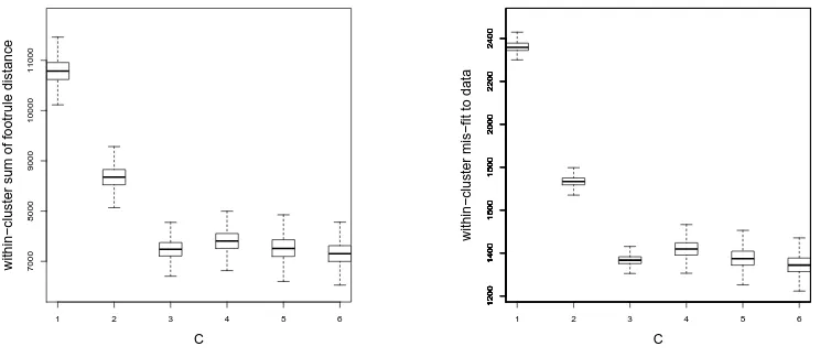
The main idea of our method for handling such data remains the same as in Section
4.1, and the algorithm is the same as Algorithm 3. However, here a “modified”
leap-and-shift proposal distribution, rather than a uniform one, is used to sample augmented ranks which are compatible with the partial ordering constraint. Suppose that, from the