* Corresponding author. Tel.: +989126794043
E-mail: [email protected] (B. Beheshti Pour) © 2013 Growing Science Ltd. All rights reserved.
doi: 10.5267/j.ijiec.2013.03.006
Contents lists available at GrowingScience
International Journal of Industrial Engineering Computations
homepage: www.GrowingScience.com/ijiec
Project selection problem under uncertainty: An application of utility theory and chance constrained programming to a real case
Behnam Beheshti Pour*, Siamak Noori and Reza Hosnavi Atashgah
Department of Industrial Engineering, Iran University of Science and Technology, Narmak, Tehran, Iran
C H R O N I C L E A B S T R A C T
Article history:
Received January 8 2013 Received in revised format March 5 2013
Accepted March 8 2013 Available online March 16 2013
Selecting from a pool of interdependent projects under certainty, when faced with resource constraints, has been studied well in the literature of project selection problem. After briefly reviewing and discussing popular modeling approaches for dealing with uncertainty, this paper proposes an approach based on chance constrained programming and utility theory for a certain range of problems and under some practical assumptions. Expected Utility Programming, as the proposed modeling approach, will be compared with other well-known methods and its meaningfulness and usefulness will be illustrated via two numerical examples and one real case.
© 2013 Growing Science Ltd. All rights reserved Keywords:
Chance constrained programming Project selection
Utility theory
1. Introduction
A common and critical issue in any organization is about how to allocate resources to candidate projects while there are som interdependencies among them. Many researchers have considered this problem for deterministic cases and one can find reliable solution for project selection problem (PSP) when all parameters are known in advance. Research and development (R&D) (Fox et al., 1984, Heidenberger & Stummer, 1999, Fang et al., 2008.), information technology (Santhanam & Kyparisis, 1996, Lee & Kim, 2001) and capital budgeting (Goldwerger & Paroush, 1977, Nemhauser & Ullmann, 2012) are some examples of application context for project selection. The real life is full of uncertainty, which makes it inevitable to devise models that are more complicated. In the context of project selection, anticipated costs, human resources and material supplies are often difficult to estimate in the planning stage. Therefore, managers must make decisions without full knowledge of some problem parameters (Medaglia et al., 2007).
mathematical frameworks. As a mathematical approach, EVM tries to optimize an expected value of objective function and, at the same time, substitutes the stochastic terms in the model constraints with their expected values. In fact, this is a simplistic approach, which does not try to manage the associated risks, adequately.
When modeling PSP, CCP tries to maintain feasibility condition (e.g. not to exceed the available budget) by forcing each constraint to hold with a predetermined confidence level (De et al., 1982; Gabriel et al., 2006). For the objective function, CCP ensures that the provided solution will yield an acceptable value again with a predetermined confidence level. Here the point is about feasibility of CCP solutions and their implications. For example, if the problem remains feasible with the probability of 95 percent, what about cases that can occur with the probability of 5 percent? In fact, we need to know whether the CCP solutions will be feasible or not after realization of some uncertain parameters. Furthermore, when deciding on confidence levels, what can the model tell the decision maker (DM) about the tradeoff between maintaining feasibility and having a better return from objective function? CCP is silent about these issues because it does not take into account the phenomenon of infeasibility occurrence (i.e. violation of stochastic constraints). With this background, Expected Utility Programming (EUP), as the proposed approach, can cope with the above issues and is capable of solving PSP appropriately under these assumptions:
1) Some parameters in PSP can be uncertain.
2) The uncertainty can be modeled via probability theory.
3) Projects are constrained linearly by their use of scarce resources (e.g., capital, labor, space requirements, and personnel, among others).
4) If the required resources for implementation of any project not to be available at a requesting time, it cannot be postponed or continued using a lower level of those resources and must be canceled (delays and partially funded projects are not allowed).
5) Project cancellations will result in some measurable outcomes (e. g. contractual obligations or loss of company credit in the market).
6) Some projects can share resources and may result in additional return if implemented together. Also technical interdependencies among projects can be included.
Although PSP has been recognized as a multiobjective problem (Ghorbani & Rabbani, 2009; Rabbani et al., 2010) and the DM may wish to simultaneously satisfy several possibly conflicting corporate goals (e. g. minimizing time-to-market and maximize economic return), here the problem will be modeled as a single objective one to keep presentation of main contributions simple. Obviously one may simply apply the proposed approach for multiobjective cases. For the same reason, only interdependencies between pairs of projects will be considered and the existence of precedence relationships will not be considered in the model. Again, all of these can be extended from the given model in a straightforward manner. The reason for paring these features from the model is that the inclusion of these features will escalate the intricacy of the solution method and we may find the solution method proposed in this work an already convoluted procedure. Besides, the proposed model suffices for handling the available data for the case study.
The reminder of this paper is organized as follow: section 2 presents the problem definition along with its parameters and the deterministic model, which remains as a basis for the stochastic model. Briefly reviewing CCP and providing some required knowledge from utility theory, section 3 presents EUP and uses two numerical examples to compare it with CCP. Section 4 contains a real case to illustrate usefulness and meaningfulness of proposed approach. Finally, section 5 summarizes the results and gives the concluding remarks.
2. Problem definition
Suppose that N projects are available for selection. These projects need M resource types and the
known in advance. Some projects have technical interdependencies while some other may share resources or produce additional returns if implemented, simultaneously. Here the required amount of each resource type for each project can be uncertain as well as the profit of projects which would be uncovered after termination. Now, the problem is: which project should be selected and started, in the absence of full knowledge, to have the best possible financial and non-financial returns while considering unpleasant events (i.e. violation of resource constraints) which may occur after realization of uncertain parameters. Note that non-financial returns should be converted such that mathematical addition, subtraction and tradeoff with financial returns make sense for the DM.
2.1. Parameters
Number of projects, , = 1,2, … ,
Number of resource types, = 1,2, … ,
The profit from implementation of project
, The additional profit from simultaneous implementation of projects and
, The amount of resource type needed for project
, , The amount of resource type that projects and can share
The amount of resource type available in the implementation stage The loss(financial and non-financial returns) from cancellation of project The set of mandatory projects
The th set of exclusive projects, = 1, 2, … ,
The set of projects that the implementing of project is contingent upon the implementation of all of them
The set of projects that the implementing of project is contingent upon the implementation of at least one of them
2.2. Decision variable
= 1,
0, ℎ
2.3. Deterministic PSP
When all parameters are known with certainty, the rational decision is to start a subset of projects such that all resource constraint to be satisfied. This way, the losses from cancellation of projects can be disregarded. The deterministic problem may be formulated as:
Model 1: deterministic model
max + (1)
subject to
, + , ≤ ∀ = 1, 2, … , (2)
= 1 ∀ ∈ (3)
≤ 1
∈
| | ≤
∈ (5)
≤
∈ (6)
∈ 0,1 ∀ (7)
The objective function given in (1) represents the total profit earned from the implementation of selected projects. Constraint (2) ensures that the amount of each resource needed for selected projects will not exceed the available amount. Constraint (3) forces the implementation of mandated projects. Constraint (4) implies that at most one project from every exclusive set may be selected. Constraint (5) indicates the situation in which implementation of project is contingent upon the execution of all of
the projects in a specific set (| | is the number of elements in the set ). Constraint (6) defines a
condition where selection of project is contingent upon implementation of at least one of the projects in a specific set ( ). Constraint (7) limits the decision variables to be binary.
3. Proposed approach and its background
3.1. A brief review of CCP
Here, we address CCP and for evaluating EVM, the reader may refer to Liu (2007). We also use CCP and EVM as a benchmark to clarify some features of EUP as the proposed method. We assume that some coefficients in the deterministic model are uncertain.
Model 2: chance constrained programming
max (8)
subject to
Pr + ≥ ≥ (9)
Pr , + , ≤ , = 1, 2, … , ≥ (10)
∈ (11)
where α and β are predetermined confidence levels, and is the -optimistic return. Constraint (11)
stands for constraints (3-7) in the deterministic problem, which can be repeated here unchanged. CCP
tries to maintain feasibility of resource constraints with a high confidence level (e.g. = .99) and
assumes that violation of constraints can be disregarded due to its very low chance of occurrence. In some cases that consequences of constraint violations are not known or are hard to estimate, CCP can be useful. In constraint (9) the DM determines his/her acceptable confidence level for objective
function, which indicates his/her attitude toward risk. If > .5 the DM is risk averse, if < .5 he is
risk seeker and = .5 models the neutral behavior.
3.2. Some required knowledge from utility theory
Assume that X is a set of “prizes” and ℓ is a lottery with payoffs in X. Lottery ℓ is a function p:
X→[0,1] such that ∑ ( ) = 1. ( )is the probability that the payoff is and when =
, , … , for some finite number n, we will write ( ) = . The expected value of a lottery is
the sum of the payoffs, where each payoff is weighted by the probability that the payoff occur (Gintis,
2009). If the lottery ℓ has payoffs , , … , with probability of , , … , , one can write ℓ =
( , ), ( , ), … , ( , ), with expected value of:
(ℓ) = (15)
Feller (1950) argued that the above equation is significant because of the law of large numbers, which states that as the number of times a lottery is played goes to infinity, the average payoff converges to expected value of the lottery with probability 1.
Assuming that individuals have consistent preferences over an appropriate set of lotteries, Von Neumann & Morgenstern (1944), Friedman & Savage (1948), Savage (1954), and Anscombe and Aumann (1963) showed that expected utility principle will be valid in stochastic environment. The final tip from utility theory, which will be of useful for our argument is utility functions. This is especially important because in practical cases, this is not generally true that one can repeat his/her choice for infinite times, and there are many cases that one can choose a lottery only one time. To model this condition, scholars have introduced different types of utility functions. The shape of utility function
depends on the risk seeking level of a specific DM. For example, ln and √ are two utility functions,
which can model risk aversion and can be used for a risk seeker DM. Therefore, the revised measure for assessing the value of a lottery, which is more accurate can be written as below:
(ℓ) = ( ), (16)
where ( ) is the utility of payoff for the DM.
3.3. The proposed approach
Consider some coefficients in the deterministic model to be uncertain. Every decision about selected subset of projects is a lottery. In the other words, for a given decision, we will have different payoffs based on realization of uncertain parameters. If after realization of uncertain parameters the resource constraints is satisfied, the payoff is the objective function in (1). Otherwise, the payoff is a combination of the profit from continued projects and the loss from cancelled ones. Here, we assume that the distribution of uncertain parameters to be discrete (if not, one can use discretization to convert continuous distributions, refer to Birge and Louveaux (1997)). To model the uncertain problem, these additional parameters can be considered:
Number of states of the world or scenarios for resource constraints,
= 1,2, … ,
, , The deterministic amount of resource type needed for project under
scenario
, , , The deterministic amount of resource type that projects and can share
under scenario
, The deterministic amount of resource type available in the
implementation stageunder scenario
, = 1, 0, ℎ
Based on Eq. (16), we construct the following model:
Model 3: Expected utility programming
max Pr( ) ( ) , + ( ) 1 − , + , , (17)
subject to
, , , + , , , , ≤ , ∀ , (18)
∈ (19)
The objective function maximizes the utility of a given decision. For every states of the world, a started project may or may not be cancelled: If continued, its profit will be earned and if cancelled the cost of its loss will be incurred. Eq. (17) implies that those projects that are not started, will not be revised after
realization of a scenario (because in such cases = 0 and so the value of objective function will be
zero for them and no profit or loss can be included). The last term in Eq. (17) ensures that an additional benefit from two synergetic projects can be earned only when they have been started already and be continued after realization of a scenario. Because all variables are binary, in every situation only a profit or a loss will be the outcome and so we have considered the utility of these parameters instead of the utility of the whole term in the accolade (the utility function is assumed to be additive). Finally, the cumulative outcomes from the projects under each state of the world have been weighted and added together. Constraint (18) ensures that in all situations the available amount of resources will not be exceeded. If after realization of uncertain parameters the required amount of resources for completion of all started projects do not be available, some projects will be cancelled so that maintain feasibility
while producing the best possible value for objective function. In fact, decision variables , are our
interface between primary decision variables and states of the world. In the other words we take a specific decision and start a subset of projects while we know that we have managed uncertainty by
, . Then after realization of scenario we will act based on , to cancel some projects if there is
any , = 0.
One may simply think that EUP works in the sense of expected value operator. This is totally wrong because EUP brings the tradeoff between feasibility of the original problem and consequences of implementation of projects (profits and losses) in a single term and uses a set of constraints, which will
hold almost surely. Note that Eq. (17) is still an uncertain term due to , and . This term should
be converted to a deterministic one based on the attitude of DM (like what was stated for CCP).
3.4. Numerical example
Here we use two very simple examples to compare EUP with CCP and EVM. Example1.
Consider the following problem with ( ) = (profit and loss are in million dollars):
2 + 3 (20)
subject to
+ ≤ (21)
where = 0,1 or 2 with probability of 1 4⁄ , 1 4⁄ and 2 4⁄ respectively. Any additional units of the scarce resource may be purchased at the price of 9 million dollars. If project 1 after selection be cancelled the cost of 4million dollars will be incurred and for the project 2 the cost of 8million dollars. Using EUP, we have:
max .25 2 , − 4 1 − , + 3 , − 8 1 − , +
.25 2 , − 4 1 − , + 3 , − 8 1 − , +
.50 2 , − 4 1 − , + 3 , − 8 1 − ,
(23)
subject to
, + , ≤ 0, , + , ≤ 1, , + , ≤ 2 (24)
, , , , , , , , , , , , , ∈ 0,1 (25)
The above model is a mixed integer programming, which can be solved very easily. The optimal
solution is = , = , = 1 with all remaining variables equal to zero. This solution states that we
should start project 1 and we have to cancel it only when tends to zero. In fact, EUP compares the utility of these four possible primary decisions:
Table 1
EUP calculations
Decision State of the world Expected utility of decision
( , ) = 2 = 1 = 0 Weighted sum
(1,1) 5 -1 -12 −3 4⁄
(1,0) 2 -4 -4 2 4⁄
(0,1) 3 -8 -8 1 4⁄
(0,0) 0 0 0 0
The only digit, which may need more attention, is -1, which represents the utility of starting both projects when tends to 1. In this case, the model compares cancelation of project 1 and 2 and decides to continue with project 2. As it was expected, the decision (1,0) is optimum. Because the cost of purchasing extra resource is 9 million dollars, it is always better to cancel projects when there is a shortage. Certainly, this is not always the case and the best method is to consider cancelation option and provision of extra resources simultaneously.
Using CCP one can write:
max 2 + 3 (26)
subject to
Pr + ≤ ≥ (27)
, ∈ 0,1 (28)
With > .75, one should not start any project, with . 50 < ≤ .75, the optimal solution is =
0, = 1 and with ≤ .50, one may start both projects. Putting aside this fact that CCP cannot
consider the cost of cancellation, one can obviously see that the quality of CCP solutions, compared with the rational approaches of utility theory, is very low. The following example, for some problems with parameters having continuous distribution, compares EUP, CCP and EVM. Although this paper addresses those problems with discrete distribution for uncertain parameters, the following example can show a feature of EUP for both discrete and continuous distribution cases.
max ( ) = , − ≤ 0 (29)
max ( ) = , − ≤ 0 (30)
max ( ) = + , − ≤ 0 (31)
max ( ) = , − ≤ 0 , − ≥ 0 (32)
where ~U[1,3], ~U[2.5,5.5]. Without considering consequence of constraint violations (i.e. the
cost of cancellation= 0), the problems will be solved by EVM, CCP and EUP. By this assumption,
although the solutions remain incomparable, it will be possible to investigate some comparable features of above modeling approaches.
Here because of the special form of problems in this example, we use the following technique to compute the EUP solutions:
max ( ) = Pr ≤ . [ ( )] +Pr > . [0] (33)
where ( ) is the expected utility of decision . The above method can be used for continuous cases
and is similar to the EUP method described earlier for discrete cases. For example for problem 3 one can write:
max ( ) = 3 −
2 . ( + ) + 0 =
3 + 2 −
2 (34)
which yield ≈ 1.87 as the optimum.
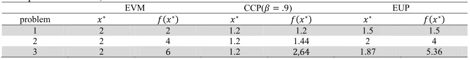
Table 2 shows the optimum solutions and optimum returns from the objective functions for the problems 1, 2 and 3, using three deferent modeling approaches.
Table 2
Comparison of EVM, CCP and EUP
EVM CCP( = .9) EUP
problem ∗ ( ∗) ∗ ( ∗) ∗ ( ∗)
1 2 2 1.2 1.2 1.5 1.5
2 2 4 1.2 1.44 2 4
3 2 6 1.2 2,64 1.87 5.36
For different objective functions, , , + , EVM and CCP have provided identical solutions ∗=
2 and ∗= 1.2, respectively. Here the optimal solution for EVM and CCP will not depend on ( ),
and only will be determined by the uncertain constraint − ≤ 0. However, when using EUP, the
tradeoff between the value earned from objective function and the probability of maintaining feasibility condition will be possible. From table 2, one can see that different decisions have been produced as a result of this feature of EUP. In fact, the other approaches have no idea about the possibility of taking a rational risk in pursuit of greater returns from objective function.
From analysis of problem (4) another feature of EUP can be observed. Using EVM, we will have:
max ( ) = , ≤ 2 , ≥ 4 (35)
Pr − ≤ 0, − ≥ 0 ≥ ⇒Pr − ≤ 0 . Pr − ≥ 0 ≥ ⇒ 3 −
2 .
− 2.5
3 ≥ ⇒
− + 5.5 − 7.5
6 ≥
(36)
The maximum of the left hand side is “. 01042” in = 2.75. Therefore, if > .01042 then there will
be no feasible solution. Here the conclusion is: by CCP one can obtain a feasible solution only with
some values of and there are many cases that using CCP yields an infeasible solution while the
original uncertain problem itself is not infeasible (for example consider problem (4) by = .9). It is
not easy to repeat the above computations for practical problems when applying CCP, therefore adjusting confidence level for obtaining a feasible solution can be a struggle. Now we solve problem (4) by EUP:
max ( ) = Pr − ≤ 0, − ≥ 0 . ( )⇒
max ( ) =− + 5.5 − 7.5
6
(37)
( )
=−3 + 11 − 7.5
6 = 0 ⇒ = 2.7613, 0.9054
(38)
and because the second derivative of ( ) in = 2.7613 is negative, this point is the maximum and
therefore is the optimum solution for the problem (4) with ( ∗) = 0.0287. Here, another feature of
EUP can be explained this way: using EUP the resulting deterministic problem will have the extermum
of ∗ such that ( ∗) = 0 only if the original uncertain problem is infeasible for all values of uncertain
parameters. Comparing with EVM, EUP never omits feasible space. Furthermore, comparing with CCP, one must find a confidence level that is acceptable for the DM and simultaneously yields a feasible space. EUP does not need such investigations and automatically provides a feasible space (if the related uncertain problem has a nonempty feasible space) and using a tradeoff between the earned value from objective function and the chance of feasibility for the solutions, EUP tries to maximize the utility of decisions.
4. A case study
Table 3
Discrete distribution of available resources
(financial resources in million dollars) 40 80 130
Pr( ) .2 .45 .35
(free hours for skilled employees) 3500 5000 6200 7800
Pr( ) .25 .35 .25 .15
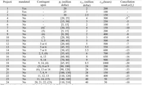
Table 4
Information for each project
Project mandated Contingent
upon (million dollar) ,dollar) (million ,
(hours) Cancellation result, ( )
1 Yes - 20 2 200 -
2 Yes - 25 3 100
-3 Yes - 30 2.5 150 -
4 No - [20, 25] 4 300 -5**
5 No - [15, 30] 3 250 -5
6 No - [5, 15] 2 100 -5
7 No (4)* [30, 35] 4 150 -10
8 No (5) [5, 15] 2 200 -5
9 No (6) [0, 20] 2 400 -8
10 No (7) [20, 30] 3 450 -9
11 No 1, 3 [40, 45] 5 500 -9
12 No 3 or 4 [20, 60] 5 500 -7
13 No 5 or 6 [45, 55] 5.5 550 -11
14 No 7 or 8 [30, 65] 5.5 600 -13
15 No 2, 5, (8) [55, 65] 6 700 -15
16 No 6, 13 [60, 80] 8 650 -16
17 No 9, 14 [70, 80] 9 900 -23
18 No 9, 14, (4) [65, 85] 8.5 1000 -20
19 No (5), 8 or 9 [80, 100] 24 200 -31
20 No (6), 13 or 14 [90, 120] 26 350 -33
21 No 7, 8, 9 [100, 130] 28 150 -45
22 No 11, 12, 13 [110, 120] 30 400 -23
23 No 11, 14, (15) [140, 180] 40 50 -17
24 No 20, 21, 22, (23) [110, 210] 40 50 -10
*When project is contingent upon ( ), it can be selected only if has not been chosen.
**For this digit, the utility of non- financial results and financial outcomes have been computed and added together.
Table 5
Information for interdependent projects
, , , , , , ,
[10, 20] [5, 15] [20, 30] [50, 80] [60, 100] [100, 110] [90, 140]
, , , , , , , , , , , , , ,
-1 -2 -3 -5 -10 -15 -20
and are assumed to be independent, so, there are 12 possible states of the worlds ( = 1, 2, … , 12)
with probability of Pr( ). Pr( ). For instance, = 12 implies that = 130 and = 7800 with
probability of Pr( = 12) = .0525.
Table 6
Utility of the results of cancellation
Credit decline very low low medium high very high
( ) -2 -5 -10 -15 -20
Internal troubles very low low medium high very high
( ) -1 -2 -5 -10 -15
as very low, low, medium, high and very high) and inter organizational disorder and dissatisfaction of people benefiting from the project(again, stated as very low, low, medium, high and very high). For the
outcomes stated as dollars, project manager decides to use ( ) = , bututility of the other results is
given in Table 6. For example if project 21 be cancelled, the loss of credit will be very high , the resulting disorder will be medium and the compensation will cost20 million dollars and the total utility can be computed as -45.
4.1. Application of EUP
Using the above information, the problem can be written as:
max Pr( ) E[ ] , + ( ) 1 − , + E , , (39)
subject to
, , , + , , , , ≤ , , = 1, … , 12 (40)
, , , ≤ , , = 1, … , 12 (41)
∈ (42)
Because the project manager expects to gain from implemented projects for several years, in Eq. (39), he has substituted the random profit of projects by their expected values. This problem has 24 primary decision variables for selection of projects and 288 secondary variables for cancellation decisions for projects under12 possible scenarios. Eq. (40) and Eq. (41) stand for 24 resource constraints, which must hold for sure. Eq. (42) ensures that all interactions among projects have been considered and all variables are limited to be binary.
4. 2. Solution method
The proposed model in this section integrates two interdependent decision phases. The first one is selection decision, which states which projects will be started. The second one is cancellation decision, which determines which started projects should be cancelled due to shortage in some resource types. Here, we have 12 independent scenarios and for each selection decision, there are 12 cancellation decisions. In fact, the cancellation decisions, for each state of the world, only depend on the set of selected projects. Therefore, one may consider the following procedure to solve the problem:
Algorithm 1
Step1: Select a set of project satisfying deterministic constraints stated in (42),
Step 2: Cancel some selected projects under each scenario and based on available resources,
Step 3: Check the stopping criterion and if confirmed go to step 4. Otherwise return to step 1,
Step 4: Stop.
the problem. Genetic algorithm (GA) is one of the modern metaheuristic algorithms and it has been successfully applied to many NP-hard problems like the knapsack problem (Lin, 2008; Alves & Almeida, 2007; Khanzadi et al., 2011).
In addition, GA has been used to solve PSP with satisfactory results compared with other available solution methods (Li et al., 2009; Ghorbani & Rabbani, 2009). GA uses the concept of evolutionary computation imitating the natural selection and biological reproduction of animal species. It originates from Darwin’s “survival of the fittest” concept, which means good parents produce better offspring. Here in algorithm 1, we use GA separately for selection decision and 12 independent cancellation decisions.
Algorithm 2
Step1: Candidate an initial population of feasible solutions using genetic algorithm respect to
constraints represented by (42),
Step 2: Simplify the objective function in (39) using proposed solution for selection decision,
Step 3: Optimize all 12 cancelation sub-problems and return the value of simplified objective function,
Step 4: Check the stopping criterion and if confirmed go to step 6. Otherwise go to step 5,
Step 5: Generate the next population using crossover and mutation operators and return to step 2.
Step 6: Stop.
More details about GA can be found in Alves & Almeida (2007), Lin (2008) and Li et al. (2009). In step 3, the sub-problems are solved to optimize the simplified objective function respect to each scenario. The following algorithm may be used for this matter:
Algorithm 3
Step1: Candidate an initial population of feasible solutions using genetic algorithm subject to resource
constraints under each scenario,
Step 2: Compute the simplified objective function,
Step 3: Check the stopping criterion and if confirmed go to step 5. Otherwise go to step 4,
Step 4: Produce the next population using crossover and mutation operators and return to step 2,
Step 5: Stop.
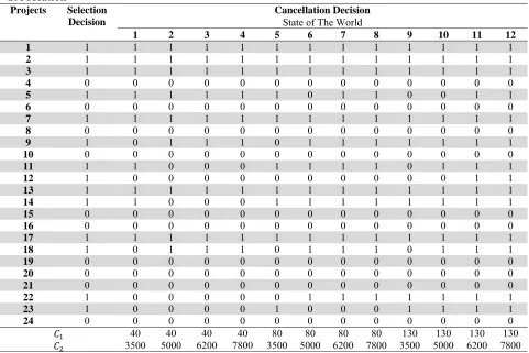
In all algorithms the stopping criterion is based on improvement in objective function, i.e. if for two successive iterations the improvement fall below a predetermined value, the algorithm will be terminated. Here, the solution method decomposes the original problem into many smaller and easier sub-problems to decrease the computation time significantly. Table 7 shows the solution provided for the case problem.
Table 7 GA solution
Projects Selection
Decision
Cancellation Decision
State of The World
1 2 3 4 5 6 7 8 9 10 11 12
1 1 1 1 1 1 1 1 1 1 1 1 1 1
2 1 1 1 1 1 1 1 1 1 1 1 1 1
3 1 1 1 1 1 1 1 1 1 1 1 1 1
4 0 0 0 0 0 0 0 0 0 0 0 0 0
5 1 1 1 1 1 1 0 1 1 0 0 1 1
6 0 0 0 0 0 0 0 0 0 0 0 0 0
7 1 1 1 1 1 1 1 1 1 1 1 1 1
8 0 0 0 0 0 0 0 0 0 0 0 0 0
9 1 0 1 1 1 0 1 1 1 1 1 1 1
10 0 0 0 0 0 0 0 0 0 0 0 0 0
11 1 1 0 0 0 1 1 1 1 0 1 1 1
12 1 0 0 0 0 0 0 0 0 0 0 1 1
13 1 1 1 1 1 1 1 1 1 1 1 1 1
14 1 1 0 0 0 1 1 1 1 1 1 1 1
15 0 0 0 0 0 0 0 0 0 0 0 0 0
16 0 0 0 0 0 0 0 0 0 0 0 0 0
17 1 1 1 1 1 1 1 1 1 1 1 1 1
18 1 0 1 1 1 0 1 1 1 0 1 1 1
19 0 0 0 0 0 0 0 0 0 0 0 0 0
20 0 0 0 0 0 0 0 0 0 0 0 0 0
21 0 0 0 0 0 0 0 0 0 0 0 0 0
22 1 0 0 0 0 0 1 1 1 1 1 1 1
23 1 0 0 0 0 1 0 0 0 1 1 1 1
24 0 0 0 0 0 0 0 0 0 0 0 0 0
40 40 40 40 80 80 80 80 130 130 130 130
3500 5000 6200 7800 3500 5000 6200 7800 3500 5000 6200 7800
5. Conclusion
This paper proposed EUP as an appropriate modeling approach for project selection problem under uncertainty and based on certain practical assumptions. It was discussed that EUP can take into account consequences of infeasibility of decisions, which might be revealed after realization of some unknown parameters. Utility theory and CCP formed the foundation of proposed approach and two numerical examples clarified some features of EUP compared to other popular modeling approaches like CCP and EVM. Finally, to show its practical meaningfulness, EUP was applied to a real case and the results were presented.
References
Alves, M. J., & Almeida, M. (2007). MOTGA: A multiobjective Tchebycheff based genetic algorithm
for the multidimensional knapsack problem. Computers & operations research, 34(11), 3458-3470.
Akbari, R., Zeighami, V., & Ziarati, K. (2011). Artificial bee colony for resource constrained project
scheduling problem. International Journal of Industrial Engineering Computations, 2(1), 45-60.
Angelelli, E., Mansini, R., & Grazia Speranza, M. (2010). Kernel search: A general heuristic for the
multi-dimensional knapsack problem. Computers & Operations Research, 37(11), 2017-2026.
Anscombe, F. J., & Aumann, R. J. (1963). A definition of subjective probability. Annals of
mathematical statistics, 34, 199-205.
Birge, J.R. & Louveaux, F. (1997). Introduction to Stochastic Programming. Springer, New York.
Charnes, A. & Cooper, W.W. (1959). Chance-constrained programming. Management Science, 6, 73–
De, P. K., Acharya, D., & Sahu, K. C. (1982). A chance-constrained goal programming model for
capital budgeting. Journal of the Operational Research Society, 33, 635-638.
Fang, Y., Chen, L., & Fukushima, M. (2008). A mixed R&D projects and securities portfolio selection
model. European Journal of Operational Research,185(2), 700-715.
Feller, W. (2008). An introduction to probability theory and its applications (Vol. 2). John Wiley &
Sons.
Fox, G. E., Baker, N. R., & Bryant, J. L. (1984). Economic models for R and D project selection in the
presence of project interactions. Management science,30(7), 890-902.
Friedman, M., & Savage, L. J. (1948). The utility analysis of choices involving risk. The Journal of
Political Economy, 279-304.
Gabriel, S. A., Kumar, S., Ordonez, J., & Nasserian, A. (2006). A multiobjective optimization model
for project selection with probabilistic considerations. Socio-Economic Planning Sciences, 40(4),
297-313.
Ghorbani, S., & Rabbani, M. (2009). A new multi-objective algorithm for a project selection
problem. Advances in Engineering Software, 40(1), 9-14.
Gintis, H. (2009). Game Theory Evolving, 2nd Ed. Princeton University Press, Princeton.
Goldwerger, J. & Paroush, J. (1977). Capital budgeting of interdependent projects: Activity analysis
and approach. Management Science, 23 (11), 1242–1246.
Heidenberger, K. & Stummer, C. (1999). Research and development project selection and resource
allocation: A review of quantitative modelling approaches. International Journal of Management
Reviews, 1 (2), 197–224.
Huang, X. (2007). Optimal project selection with random fuzzy parameters. International Journal of
Production Economics, 106, 513–522.
Khanzadi, M., Soufipour, R., & Rostami, M. (2011). A new improved genetic algorithm approach and a competitive heuristic method for large-scale multiple resource-constrained project-scheduling
problems. International Journal of Industrial Engineering Computations, 2(4), 737-748.
Kumar, R. & Singh, P.K. (2010). Assessing solution quality of biobjective 0-1 knapsack problem using
evolutionary and heuristic algorithms. Applied Soft Computing, 10, 711–718.
Lee, J. W. & Kim, S. H. (2001). An integrated approach for interdependent information system project
selection. International Journal of Project Management, 19, 111-118.
Lin, F. (2008). Solving the knapsack problem with imprecise weight coefficients using genetic
algorithms. European Journal of Operational Research, 185, 133–145.
Li, Y.F., Xie, M. & Goh, T.N. (2009). A study of project selection and feature weighting for analogy
based software cost estimation. Journal of Systems and Software, 82, 241–252.
Liu, B. (2007). Theory and Practice of Uncertain Programming. 2nd ed. Tsinghua University, Beijing.
Medaglia, A. L., Graves, S. B. & Ringuest, J. L. (2007). A multiobjective evolutionary approach for
linearly constrained project selection under uncertainty. European Journal of Operational Research,
179, 869–894.
Nemhauser, G.L. & Ullmann, Z. (2013). Discrete dynamic programming and capital allocation.
Management Science, 15 (9), 494–505.
Neumann, V., Morgenstern, J. & Morgenstern, O. (1944). Theory of Games and Economic Behavior.
Princeton University Press, Princeton.
Rabbani, M., Aramoon Bajestani, M. & Baharian Khoshkhou, G. (2010). A multi-objective particle
swarm optimization for project selection problem. Expert Systems with Applications, 37, 315–321.
Santhanam, R. & Kyparisis, G.J. (1996). A decision model for interdependent information system
project selection. European Journal of Operational Research, 89, 380–399.