Published by Central Fisheries Research Institute (SUMAE) Trabzon, Turkey in cooperation with Japan International Cooperation Agency (JICA), Japan
R E S E A R C H P A P E R
Determination of Spatial and Temporal Changes in Water
Quality at Asi River Using Multivariate Statistical Techniques
Ece Kilic
1,* , Nebil Yucel
11İskenderun Technical University, Faculty of Marine Sciences and Technology, Department of Water Resources
Management and Organization, Hatay-Turkey.
Article History
Received 08 March 2018 Accepted 28 August 2018 Early View 31 August 2018
Corresponding Author
Tel.: +903266141693 E-mail: [email protected]
Keywords
Orontes River
Environmental impact assessment Cluster analysis
Discriminant analysis Principal component analysis
Abstract
Water quality in surface waters is a critical issue since they are used in domestic, agricultural and industrial purposes. Therefore, proper water management strategies should be taken care of to protect water bodies. To accomplish this goal, ten years (2004-2014) seasonal water quality monitoring results consisting of 16 parameters (BOD5, COD, DO, NO2-, NO3-, NH4+, PO42-, SO42-, EC, SS, TDS, T, Na+, Mg2, Ca2+,Q )
measured at 5 stations taken from State of Hydraulic Works of Turkey was examined using multivariate statistical techniques like cluster analysis (CA), discriminant analysis (DA) and principal component / factor analysis (PCA/FA). Hierarchical CA grouped 5 monitoring stations and 4 seasons into two clusters as polluted/less polluted area and wet/dry season, respectively. DA showed that parameters responsible for temporal change in Asi River are Na+, Mg2+, Ca2+, Q, BOD, NH4+ and SS
with 92.2% accuracy. Likewise, SO42-, DO and T were found as parameters responsible
for temporal change with 90% accuracy. PCA revealed that mineral pollution, nutrient pollution, and organic pollution are major latent factors which influence the water quality of Asi River. It also showed that erosion, agricultural activities, domestic and industrial discharges are fundamental causes of water pollution in the study area. To conclude, the study revealed that multivariate statistical methods are beneficial tools for the evaluation of complex datasets like water quality monitoring data.
Introduction
Surface waters are primary and limited water resources to meet agricultural, industrial and domestic water needs of human and living beings. They also play an important role in the transport and assimilation of domestic and industrial wastewater as well as agricultural runoff (Zhou, Liu, & Guo, 2007a). This situation makes surface water vulnerable to pollution. Surface water quality is depended on both anthropogenic activities like urban, agricultural, industrial activities which are spatial and have continuous impacts on the environment and natural processes like precipitation rate, weathering processes, soil erosion which are temporal and climate depended
(Giri & Singh, 2014). Therefore, determination of water quality in surface waters is a problematic matter and require monitoring studies. However, monitoring studies often result in complex and huge datasets and interpretation of water quality from these results is difficult due to latent interrelationships between measured parameters (Zhou, Guo, Liu, & Jiang, 2007b; Ruždjak & Ruždjak, 2015).
to extract meaningful information from long-monitoring study results. CA helps a researcher to cluster (group) a set of variables in such a way that similar variables are perched in a same cluster. DA is widely applied to assess the adequacy of classification between clusters. Lastly, PCA/FA is a dimension-reduction tool that is used to reduce large set of variables into smaller ones that are still contain most of the meaningful information in the large set.
These multivariate statistical techniques are widely applied in environmental monitoring datasets because, (1) they reflect multivariate nature of the system more accurately, (2) provide a way to handle large data sets and (3) provide a means of detecting and quantifying multivariate patterns that arise out of the correlation structure of variable set (McGarigal, Cushman, & Stafford, 2000; Boyacioglu & Boyacioglu, 2008). Studies conducted in this field indicated that multivariate statistical analysis are widely accepted and effective tools in the identification of water quality status of ecological systems, in the evaluation of spatial and temporal variations in surface waters and in the identification of latent factors causing water pollution (Singh, Malik, & Sinha, 2005; Shrestha & Kazama, 2007; Zhou et al., 2007a; Wang, Liu, Liao, & Lee, 2014; Azhar, Aris, Yusoff, Ramli, & Juahir, 2015; Ogwueleka, 2015; Muangthong & Shrestha, 2015; Jung et al., 2016; Monica & Choi, 2016; Chow et al., 2016; Zheng, Yu & Wang, 2016). However, there are very few studies conducted in Turkey’s surface waters for the evaluation of spatial and temporal variations (Boyacioglu & Boyacioglu, 2008; Ödemis, Sarıgün & Evrendilek, 2010). Also, even though there are some studies in Asi River which aim to investigate water quality (Taşdemir & Göksu, 2001; Ağca, Ödemiş &Yalçın, 2009), they are not proper for the investigation of spatiotemporal changes in an integrated way.
Therefore, monitoring data obtained from State Water Works (DSİ) of Turkey covering the year from 2004 to 2014 based on query pattern was analyzed using CA, DA and PCA/DA. The objective of the present study is (1) to evaluate current water quality status of Asi Basin, (2) to understand significant parameters responsible for temporal and spatial variation, (3) to identify similarities between monitoring periods and stations and to identify pollution sources in the study area.
Materials and Methods
Study Area
Asi River is a transboundary river and its water is shared among Lebanon, Syria, and Turkey. The river rises in the mountains of Lebanon and flows 40 km in Lebanon to continue into the Syrian for about 325 km before arriving in Turkey for its last reach of 88 km to the Mediterranean Sea (FAO, 2009). The Asi Basin is
located in the Mediterranean climate zone where the summers are hot and arid, and the winters are warm and rainy. Watershed has an average annual precipitation of 816 mm, an average temperature of 16.8°C, an annual total flow of 1,17 km³ / year (TUBİTAK MAM, 2013). Main anthropogenic activities carried out in the Asi Basin are agriculture, animal husbandry, and agriculture-based industries. Therefore, the river is subjected to the various kinds of point and diffuse pollution sources. The figure representing the study area is given Figure 1.
Water Quality Data and Pretreatment
Water quality monitoring data covers 16 different parameters which are biological oxygen demand (BOD5), chemical oxygen demand (COD), dissolved
oxygen (DO), nitrite (NO2-), nitrate (NO3-), ammonia
(NH4), dissolved phosphate (PO4), sulfate (SO42-),
electrical conductivity (EC), suspended solids (SS), total dissolved solids (TDS), water temperature (T), sodium ion (Na+), magnesium ion (Mg2+), calcium ion (Ca2+),
flowrate (Q) measured at 5 different stations analyzed using multivariate statistical methods for the determination of spatio-temporal variations in Asi River. Samandağ, Antakya, Eşrefiye and Demirköprü stations are located at the main stream of Asi River. Former two stations are near the urbanized areas; whereas, latter two are located inside agricultural areas. Different from other stations, Küçük Asi station is located at the tributary of Asi River. This tributary is important because it reflects the impact of Amik Plain on the river quality. Figure 1 represents monitorıng stations with CORINE 2012 land use map.
Measurement of water quality parameters was carried out at the accredited laboratory of State of Hydraulic Works of Turkey. BOD, COD, TDS measurement were done using standard methods (SM 5210, SM 5220 B, SM 2540C, respectively). DO measurement was carried out with electrochemical probe method (TS EN ISO 5814). NO2-, NO3-, PO4
measurement were carried out by ion chromatography in accordance with TS EN ISO 10304-1 standards. NH4,
Na+, Mg2+, Ca2+ measurement were done with ion
chromatography in accordance with TS EN ISO 14911 standards. SO42-, EC, and SS analysis was done with
iodometric method, electrode method and gravimetric method in accordance with SM 4500-S2-F, TS 9748 EN
27888 and TS EN 872 standards, respectively.
BOD5 is defined as the amount of oxygen required
support balanced aquatic environment (Synder, 2007). Nitrogen compounds are the indicators of diffuse pollution since they are usually found in effluents of agricultural drainage waters (Ogwueleka, 2015). In addition, they decrease primary production in a water body and may cause eutrophication problem (Aksoy, Bulut, & Yenilmez, 2006). Dissolved phosphate amount in water is important since it is essential for photosynthesis (Froelich, 1988). Therefore, excess amount of it will support the algal development and may lead to eutrophication. SO42- accelerates the
dissolution of nutrients found in sediments into surface waters (Orem, 2011). EC shows electric conductivity of water and as the amount of dissolved ion increases, its value increases (Anonymous, 2016). SS may comprise both organic and inorganic matter like plankton, silt, clay (Ell, 2008). TDS is a measure of total dissolved solids found in water. Na+, Mg2+, Ca2+ are the most
common alkali metals found in surface waters (Grochowska & Tandyrak, 2009). They usually reach water bodies due to dissolution of rocks found in watershed structure (Gałczyńska, Gamrat, Burczyk, Horak, & Kot, 2013).
Before applying any multivariate statistics to the dataset, it was visualized using scatter graphs to exclude extreme values. Thereafter, all missing data were replaced with yearly average values. Since multivariate statistical tools require confirmation of normal distribution, the normality of each variable was checked by using Kolmogrov-Smirrow (K-S) z test (Muangthong & Shrestha, 2015). Then, for DO and T
square transformation, for Na+ square root
transformation and for other parameters logarithmic transformation was applied to satisfy normal distribution assumption. To analyze whether or not the dataset is suitable for PCA/FA, Kaiser-Mayer-Olkin (KMO) and Barlett’s test were performed. KMO is a measure of sampling adequacy that indicates the proportion variance (Ogwueleka, 2015). KMO results greater than 0.5 obtained in this research shows that data set is suitable for PCA/FA. Barlett’s test of sphericity indicates whether correlation matrix is an identity matrix or not. Lastly, DA was applied to normalized data, whereas CA and PCA were applied to normalized data that was standardized through z-scale transformation to avoid misclassifications arising from the different orders of magnitude of both numerical values and variance of the parameters analyzed (Lei, 2013).
Cluster Analysis
CA is a beneficial tool which helps explication of large and multidimensional datasets like environmental data (Cieszynska, Wesolowski, Bartoszewicz, Michalska, & Nowacki, 2012). Cluster analysis help researcher to group water samples resulting in high interval (within clusters) homogeneity and high external (between clusters) heterogeneity (Shrestha & Kazama, 2007). Hierarchical agglomerative clustering is the widely used approach to analyze similarity between sample and entire dataset (McKenna, 2003). The Euclidean distance
is widely used distance coefficient, which measures the similarity between two samples and a distance that can be represented by the difference between analytical values from both the samples (Otto, 1998). Result of cluster analysis is usually given with a tree like diagram called dendrogram, which visualizes the summary of clustering process with a considerable reduction in dimensionality of the original data (Shrestha & Kazama, 2007). In this study, hierarchical agglomerative CA was performed on the normalized data set by means of Ward's method, using Euclidean distances as a measure of similarity.
Discriminant Analysis
DA is a method of analyzing dependence that is a special case of canonical correlation, and one of its objectives is to determine the significance of different variables, which can allow the separation of two or more naturally occurring groups (Zhou et al., 2007b). The DA constructs a discriminant function for each group (Johnson & Wichern, 1992; Wunderlin, Wesolowski, Bartoszewicz, Michalska & Nowacki, 2001) as in the equation below:
f(Gi) = ki+ ∑nj=1wijpij (1)
where i is the number of groups (G), ki is the constant inherent to each group, n is the number of parameters used to classify a set of data into a given group, wj is the weight coefficient, assigned by DA to a given selected parameter (pj).
DA was used on normalized data matrix using standard modes for the construction of discriminant functions to evaluate spatiotemporal variations in Asi River (Wang et al., 2014). Monitoring stations and seasons were the grouping variables, all the measured parameters were the independent variables.
Principal Component Analysis
The main goal of factor analysis is to explain the covariance relationships among a large number of variables with the help of the least number of random variables (Johnson & Wichern, 1992). The most widely used method of obtaining factors is principal component analysis (Kalaycı, 2016).
PCA is designed to transform the original variables into new, uncorrelated variables (axes), called the principal components (PCs), which are linear combinations of the original variables (Shrestha & Kazama, 2007). PC provides information on the most significant parameters which describes the whole dataset without losing any information (Helena et al., 2000). Therefore, it allows the identification of latent factors depending on pollution sources and its origins like anthropogenic sources (industrial and domestic discharges etc.) or natural sources (climate, erosion etc.) (Kowalkowskia, Zbytniewskia, Szpejnab &
Buszewki, 2006). Equation which describes principal components mathematically is given below:
zij= ai1x1j+ ai2x2j+ ai3x3j+ ⋯ + aimxmj (2)
Where z is the component score, a is the component loading, x the measured value of a variable, i is the component number, j the sample number and m the total number of variables.
To reduce the contribution of less significant parameters on data structure obtained after PCA, FA was conducted by rotating the axis defined by PCA, according to well established rules. At the end of the FA, new variables called varifactors (VF) were obtained. The main difference between PC and VF is that while PC is a linear combination of observable water quality variables, VF can include unobservable, hypothetical, latent variables (Vega, Zbytniewskia, Szpejnab & Buszewki, 1998, Helena et al., 2000). The equation representing the factor analysis is given below:
zfj= af1f1i+ af2f2i+ af3f3i+ ⋯ + afmfmi+ efi (3)
Where z is the measured variable, a is the factor loading, f is the factor score, e is the residual term accounting for errors or another source of variation, i is the sample number and m is the total number of factors.
Results and Discussion
Preliminary Assessment of Water Quality
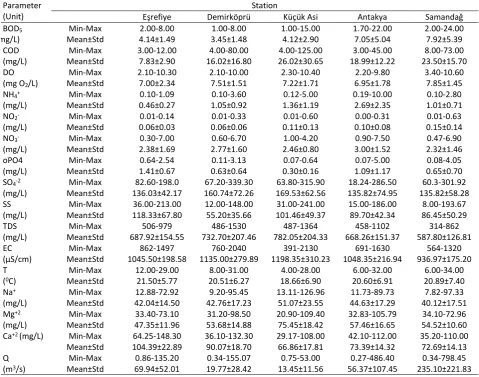
Descriptive statistic tools and two-way ANOVA test was used for the preliminary assessment of water quality in Asi River. Table 1 indicates the basic statistic of water quality dataset.
Descriptive statistics indicate that most of the parameters have high standard deviation and high change interval. Therefore, it can be said that water quality in Asi River is time and space depended because of the natural and anthropogenic processes carried out in the watershed (Gonzalez, Almeida, Calderón, Mallea, & González, 2014).
When average values of water quality parameters compared with Water Pollution Control Regulation of Turkey, it is found that Asi River is suffered from oPO4
3-, NH4+ and NO2- pollution. This indicates that Asi River
has high organic pollution since nitrogen compounds in surface waters usually related to organic pollution (Yang, Shen, Zhang, & Wang, 2007). Also, severe oPO4
3-pollution indicates the impact of agricultural diffuse water and domestic discharges (Wu, 2005).
Two way ANOVA test was performed to determine the existence of spatial and temporal variation in the dataset. It showed that TDS, SO42-, Ca2+,
Q parameters were changing both temporally and spatially (P<0.05). BOD5, COD, NH4, NO2, oPO4, SS, EC,
and DO vary only seasonally (P<0.05). As a result, both descriptive statistics and two way ANOVA test confirmed the existence of the spatiotemporal change in water quality of Asi River. However, since these methods are insufficient to explain correlations between parameters in complex datasets (Vega et al., 1998), multivariate statistics were used to analyze water quality changes in detail.
Temporal/Spatial Similarities and Grouping
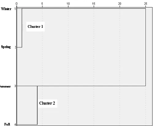
Temporal CA generated a dendrogram, grouping 4 seasons into 2 clusters. Cluster 1 comprised winter and spring indicating wet season, high flow, whereas; cluster 2 comprised summer and fall season indicating dry season, low flow (Figure 2). Therefore, water quality in Asi River is influenced by the local climate and similar results can be found on literature (Ogwueleka, 2015; Zhang, Guo, Meng, & Wang, 2009).
Spatial CA generated a dendrogram, grouping 5 stations into 2 clusters. Cluster 1 comprised Eşrefiye and Demirköprü stations, whereas; cluster 2 comprised Küçük Asi, Antakya and Samandağ stations (Figure 3). While Demirköprü and Eşrefiye stations are located near the agricultural land; Küçük Asi, Antakya ve
Samandağ stations are locations where urbanizations begin in addition to agricultural activities. Therefore, it can be said that first cluster is suffered from agricultural diffuse pollution more severely than second one. So, like Boyacioglu and Boyacioglu (2008) study, it is concluded that water quality similarities are highly depended on land use in Asi watershed.
As it can be seen from Figure 3, linking distance between Küçük Asi station with Antakya and Samandağ stations is the greatest distance in the dendrogram. Küçük Asi station is located at the downstream of Amik plain. As a result of agricultural activities taking care of at the plain, inorganic pollution is a great concern in the surface waters in addition to organic pollution. On the other hand, Antakya and Samandağ stations are located near the urbanized land and suffered from domestic discharges, industrial discharges as well as agricultural pollution. As a result, it can be said that even though Küçük Asi, Antakya and Samandağ stations are similar in the aspect of water quality, main pollution sources are different from each other. Results indicate that cluster analysis is applicable to large water quality datasets for the examination of similarities in the monitoring area (Zhou et al., 2007, Muangthong & Shresta, 2015, Zheng et al., 2016).
Table 1. Descriptive Statistics of Water Quality Data
Parameter (Unit)
Station
Eşrefiye Demirköprü Küçük Asi Antakya Samandağ
BOD5
(mg/L)
Min-Max 2.00-8.00 1.00-8.00 1.00-15.00 1.70-22.00 2.00-24.00
Mean±Std 4.14±1.49 3.45±1.48 4.12±2.90 7.05±5.04 7.92±5.39
COD (mg/L)
Min-Max 3.00-12.00 4.00-80.00 4.00-125.00 3.00-45.00 8.00-73.00 Mean±Std 7.83±2.90 16.02±16.80 26.02±30.65 18.99±12.22 23.50±15.70 DO
(mg O2/L)
Min-Max 2.10-10.30 2.10-10.00 2.30-10.40 2.20-9.80 3.40-10.60
Mean±Std 7.00±2.34 7.51±1.51 7.22±1.71 6.95±1.78 7.85±1.45
NH4+
(mg/L)
Min-Max 0.10-1.09 0.10-3.60 0.12-5.00 0.19-10.00 0.10-2.80
Mean±Std 0.46±0.27 1.05±0.92 1.36±1.19 2.69±2.35 1.01±0.71
NO2-
(mg/L)
Min-Max 0.01-0.14 0.01-0.33 0.01-0.60 0.00-0.31 0.01-0.63
Mean±Std 0.06±0.03 0.06±0.06 0.11±0.13 0.10±0.08 0.15±0.14
NO3
-(mg/L)
Min-Max 0.30-7.00 0.60-6.70 1.00-4.20 0.90-7.50 0.47-6.90
Mean±Std 2.38±1.69 2.77±1.60 2.46±0.80 3.00±1.52 2.32±1.46
oPO4 (mg/L)
Min-Max 0.64-2.54 0.11-3.13 0.07-0.64 0.07-5.00 0.08-4.05
Mean±Std 1.41±0.67 0.63±0.64 0.30±0.16 1.09±1.17 0.65±0.70
SO4-2
(mg/L)
Min-Max 82.60-198.0 67.20-339.30 63.80-315.90 18.24-286.50 60.3-301.92 Mean±Std 136.03±42.17 160.74±72.26 169.53±62.56 135.82±74.95 135.82±58.28 SS
(mg/L)
Min-Max 36.00-213.00 12.00-148.00 31.00-241.00 15.00-186.00 8.00-193.67 Mean±Std 118.33±67.80 55.20±35.66 101.46±49.37 89.70±42.34 86.45±50.29 TDS
(mg/L)
Min-Max 506-979 486-1530 487-1364 458-1102 314-862
Mean±Std 687.92±154.55 732.70±207.46 782.05±204.33 668.26±151.37 587.80±126.81 EC
(µS/cm)
Min-Max 862-1497 760-2040 391-2130 691-1630 564-1320
Mean±Std 1045.50±198.58 1135.00±279.89 1198.35±310.23 1048.35±216.94 936.97±175.20 T
(0C)
Min-Max 12.00-29.00 8.00-31.00 4.00-28.00 6.00-32.00 6.00-34.00 Mean±Std 21.50±5.77 20.51±6.27 18.66±6.90 20.60±6.91 20.89±7.40 Na+
(mg/L)
Min-Max 12.88-72.92 9.20-95.45 13.11-126.96 11.73-89.73 7.82-97.33 Mean±Std 42.04±14.50 42.76±17.23 51.07±23.55 44.63±17.29 40.12±17.51 Mg+2
(mg/L)
Min-Max 33.40-73.10 31.20-98.50 20.90-109.40 32.83-105.79 34.10-72.96 Mean±Std 47.35±11.96 53.68±14.88 75.45±18.42 57.46±16.65 54.52±10.60 Ca+2 (mg/L) Min-Max 64.25-148.30 36.10-132.30 29.17-108.00 42.10-112.00 35.20-110.00
Mean±Std 104.39±22.89 90.07±18.70 66.86±17.81 73.39±14.32 72.69±14.13 Q
(m3/s)
Figure 2. Dendrogram generated as a result of Temporal CA.
Figure 3. Dendrogram generated as a result of Spatial.
Temporal and Spatial Variations in Water Quality
Temporal DA was applied to the normalized dataset after dividing the dataset into two clusters (dry and wet season) resulted in CA. Discriminant functions are obtained using forward stepwise method in which variables are included step by step beginning with the more significant until no significant changes are obtained. Temporal DA results indicated that dissolved oxygen, SO42- and T are the most significant parameters
to discriminate between wet and dry seasons (Table 2). Main source of sulfate in the surface waters is mineral containing soils. Therefore, during periods when precipitation was abundant, sulfate was dissolved from the soil and reached the Asi River with surface runoff. Since the solubility of oxygen in water is inversely proportional to temperature (Shrestha & Kazama, 2007), decrease in dissolved oxygen content during the dry season (high temperature) is expected.
Spatial DA results indicated that Na+, Mg2+, Ca2+,
Q, BOD, NH4+ and SS parameters are the most
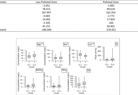
significant parameters to discriminate between polluted and less polluted areas (Table 3). In other words, these 7 parameters are responsible for most of the expected the variation through Asi River. Box and whisker plots belonging to these parameters are given below Figure 4.
As it can be seen from Table 2 most significant parameters according to discriminant function coefficients are Mg2+, Ca2+ and SS. Mg2+ concentration
is greater in the second cluster (polluted zone) due to the surface flow which has a high salt content (Ağca et al., 2009) coming from Amik Plain. SS concentration variation is in a similar trend with Mg2+. This indicated
the effect of erosion. Contrary to Mg2+ concentration,
Ca+ concentration is greater at the first cluster (less
zones (Zwahlen, Gonzalez, & Asaad, 2014). Therefore, the lime found in the soil structure dissolves during rainy weathers and reaches the Asi River with surface flow.
Data Structure Determination and Source Identification
PCA is applied on standardized normalized dataset separated as polluted and less polluted area based on cluster analysis results to identify main pollution factors that influenced each identified regions (Zhang et al., 2009; Monica & Choi, 2016). In order to understand the applicability of PCA on the dataset, Barlett and KMO tests were applied. KMO and Barlett sphericity test results of the less polluted region consisting of Eşrefiye and Demirköprü stations were found as 0.599 and 0.00, respectively. Similarly, KMO and Barlett sphericity test results of the polluted region consisting of Küçük Asi, Antakya and Demirköprü stations were found as 0.595 and 0.00, respectively. Results indicated that PCA could achieve a significant reduction of dimensionality of the original dataset.
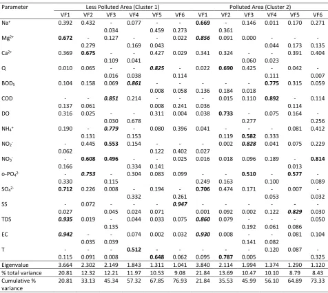
Factor analysis of two datasets belonging to polluted and less polluted regions resulted in 6 variance factors (VFs) with eigenvalues greater than 1 and explained 77% and 73% of total variance, respectively. An eigenvalue gives a measure of the significance of the factor and eigenvalues greater than 1 are considered as significant (Kim & Mueller, 1987; Muangthong & Shrestha 2015). Corresponding VFs, variable loadings and explained variance are given at Table 4. Liu, Lin, & Kuo (2003), classified loadings greater than 0.75 as strong, loadings between 0.75-0.50 moderate and loadings smaller than 0.5-0.3 as weak.
Less Polluted Region
Among six VFs obtained for the less polluted region, VF1 explained 20.8% of total variance and had strong positive loading on TDS, EC and moderate positive loading on Mg2+ and SO
42-.TDS and EC indicate
soil erosion occurring depending on seasonal storms (Kowalkowskia et al., 2006). Similarly, SO42- reaches to
the surface water due to the dissolution of lime found in soil (Vega et al., 1998). Also, Mg2+ is commonly found
in agricultural drainage water (Boyacioglu, 2006). Therefore, this factor represents mineral pollution caused by seasonal storms. VF2 explained 12.3% of total variance and had moderate positive loading on Ca2+, NO
3-, oPO42-. While NO3- and oPO42- indicates
diffused pollution resulted from agricultural activities (Ogwueleka, 2015), Ca2+ found in surface waters could
be mainly due to natural processes like ion exchange between soil and water interface and dissolution from soil. (Guo & Wang, 2004). So, VF2 showed that nutrient pollution resulted from both anthropogenic and natural processes. VF3 explained 12.2% of total variance and
had positive strong NH4-, COD, and positive moderate
NO2-, NO3- loadings. Since fertilizers used in agricultural
activities are the main sources of nitrogenous compounds in surface waters (Ogwueleka, 2015), VF3 represents diffuse agricultural pollution. Additionally, VF4 had positive strong BOD5 and positive negative T
loading and explained 12% of total variance. BOD5 is an
index indicating organic pollution resulted from domestic and industrial discharges ( Kazi et al., 2009; Juahir et al., 2011). VF5 explained 10.5% of total variance and contained positive strong Q and negative moderate T loading. The inverse relationship between Q and T is a result of weather condition of the studied area. As temperature increases during dry season, evaporation increases, as a result; surface flow decreases. So, this factor represents the impact of seasonal change on surface water. Lastly, VF6 explained 9.1% of total variance and had positive strong SS loading. This factor represents diffuse pollution due to soil erosion (Muangthong & Shresta 2015, Chow et al., 2016).
Polluted Region
VF1 explained 21.8% of total variance and has positively strong Mg2+, TDS, EC and positively moderate
Na+ and SO
42- loadings. So, this factor points out the
dissolution of minerals from soil. VF2 explained 10.5% of total variance and had positive moderate Q, DO and negative moderate T loading. As mentioned before, there is a negative correlation between T and Q as a result of evaporation. Additionally, as temperature of the water increases, dissolution of oxygen in water decreases (Wang et al., 2013). As a result, VF2 is related to seasonal change and had natural causes. VF3, on the other hand; explained 10.5% of total variance and had positive strong NO2-, positive
moderate oPO4 and negative moderate NH4+.
Therefore, this factor indicated nutrient pollution from agricultural runoff (Sing et al., 2005). VF4 contained positive strong BOD5 and COD loadings and explained
10.1% of total variance. BOD5 and COD are indicators of
organic pollution from industrial and domestic discharges (Kazi et al., 2009). VF5 had positive moderate oPO4 and negative strong SS loading and
explained 9% of total variance. The inverse relationship between oPO4and SS indicates that pollution at the
studied area is a result of anthropogenic activities. Finally, VF6 explained 9% of total variance and had positive strong NO3- loading. The presence of nitrate
was due to fertilizers used in crop cultivation which was carried by surface runoff.
Table 2. Classification function coefficients for temporal discriminant analysis
Parameter Wet Season Dry Season
DO 0.088 0.015
SO4-2 61.527 58.068
T 0.021 0.031
(Constant) -74.804 -67.971
Table 3. Classification function coefficients for spatial discriminant analysis
Parameter Less Polluted Zone Polluted Zone
Na+ -2.651 -1.891
Mg2+ 78.413 89.618
Ca2+ 187.997 163.354
Q -4.683 -2.772
BOD 14.062 17.854
NH4+ -3.344 .166
SS 45.251 50.401
(Constant) -286.694 -276.921
Figure 4. Box and whisker plots of water quality parameters responsible for spatial change.
provide significant data reduction, it helped to identify pollution sources specific to Asi River. Same situation is true in Sing et al. (2005) and Nie, Li, Jiang, Diao, & Li (2015) studies.
Conclusion
In this study, multivariate statistical techniques were used to identify spatial and temporal changes in water quality at Asi River. Cluster analysis grouped both the sampling stations and seasons into two clusters as polluted / less polluted areas and wet / dry seasons. DA was used to determine most significant parameters among groups separated by CA. DA showed that parameters responsible for temporal change in Asi River are Na+, Mg2+, Ca2+, Q, BOD, NH
4+
and SS with 92.2% accuracy. Likewise, SO42-, DO and T
were found as parameters responsible for temporal change with 90% accuracy. PCA/FA helped to identify latent pollution factors/ sources; but, it did not provide considerable data reduction. Pollution indicating
parameters for less polluted and polluted region were TDS, EC, SO42-, COD, BOD5, SS and TDS, EC, Mg2+, NO2-,
NO3-, respectively. Also, pollution sources were
identified as erosion, agricultural activities, domestic and industrial discharges and dissolution of minerals. Among all these pollution sources, diffuse pollution is dominant in the area as a result of natural processes especially dissolution and transport of minerals and solid particles with surface runoff and agricultural activities. High positive NO2-, NO3- and PO42- loadings
Asi River. Also, it showed that multivariate statistical techniques are effective in the investigation of water quality datasets.
Acknowledgements
This study is conducted with the support of Mustafa Kemal University, coordination of scientific research projects in the framework of project number 14781.
References
Ağca, N., Ödemiş, B., & Yalçin, M. (2009). Spatial and temporal variations of water quality parameters in Orontes river (Hatay, Turkey). Fresenius Environmental
Bulletin, 18 (4), 456-460
Aksoy, A., Bulut, E., &Yenilmez, F. (2006). Uluabat Gölü Ötrofikasyon Kontrolü için Maksimum Alıcı Ortam Fosfor Yüklerinin Belirlenmesi. TÜBİTAK Deniz Bilimleri ve Çevre Araştırmaları Grubu Projesi, Ankara, Türkiye,
105 pp
Anonymous. (2016). Water Quality Indicators: Conventional Variables. Retrieved from http://www.ramp-alberta.org/river/water+sediment+quality/chemical/co nventional.aspx
Azhar, S.C., Aris, A.Z., Yusoff, M.K., Ramli, M.F., & Juahir, H. (2015). Classification of river water quality using multivariate analysis. Procedia Environmental Sciences,
30,79-84.
https://doi.org/10.1016/j.proenv.2015.10.014
Boyacioglu, H. (2006). Surface water quality assessment using factor analysis. Water SA, 32(3), 389-393. http://dx.doi.org/10.4314/wsa.v32i3.5264
Boyacioglu, H., & Boyacioglu, H. (2008). Water pollution sources assessment by multivariate statistical methods in the Tahtali Basin, Turkey. Environmental Geology,
54(2), 275-282. https://doi.org/10.1007/s00254-007-0815-6
Chow, M. F., Shiah, F. K., Lai, C. C., Kuo, H. Y., Wang, K. W., Lin, C. H., Chen T.Y., Kobayashi Y. & Ko, C. Y. (2016). Evaluation of surface water quality using multivariate statistical techniques: a case study of Fei-Tsui Reservoir basin, Taiwan. Environmental Earth Sciences, 75(1),
1-Table 4. Loadings of water quality parameters on significant principle components
Parameter Less Polluted Area (Cluster 1) Polluted Area (Cluster 2)
VF1 VF2 VF3 VF4 VF5 VF6 VF1 VF2 VF3 VF4 VF5 VF6
Na+ 0.392 0.432
-0.034
0.077
-0.459 -0.273
0.669
-0.361
0.146 0.011 0.170 0.271
Mg2+ 0.672
-0.279
0.127
-0.169 -0.043
0.022 0.856 0.091 0.000
-0.044 -0.173
-0.135
Ca2+ 0.369 0.675
-0.109 -0.041
0.427 0.029 0.341 0.324
-0.060 -0.023
0.391 0.404
Q 0.010 0.065
-0.016 -0.038
0.825
-0.114
0.022 0.690 0.425
-0.111
0.042
-0.007
BOD5 0.104 0.158 0.069 0.861
-0.008 -0.058 -0.136 -0.184 -0.018
0.775 0.315 0.059
COD
-0.137 -0.061
0.851 0.214
-0.008 -0.241
-0.036
0.015 0.110 0.892
-0.114 0.114
DO 0.316 0.025
-0.030 -0.678
0.311 0.004 0.038 0.733
-0.277
0.075 0.164
-0.256
NH4+ 0.190
-0.131
0.779
-0.153
0.080 0.396 0.041
-0.119 -0.582
-0.333
0.081 0.412
NO2-
-0.062
0.445 0.553 0.154
-0.122 -0.402
-0.027
0.002 0.828 0.041 0.075 0.229
NO3-
-0.166
0.608 0.496
-0.334 -0.141
0.025 0.016 0.018 0.096 0.189
-0.013 0.814
o-PO42-
-0.330
0.753
-0.115
0.304 0.083 0.099
-0.249 -0.163
0.510
-0.100
0.577
-0.089
SO42- 0.712 0.226 0.008
-0.332
0.194
-0.261
0.706 0.474 0.171
-0.053
0.007
-0.032
SS
-0.027
0.072
-0.045 -0.024
-0.071
0.947
-0.001 -0.092 -0.002 -0.122 -0.829 -0.030
TDS 0.935 0.019
-0.135
0.044 0.033 0.075 0.860 0.079
-0.192 -0.061 -0.086 0.050
EC 0.942
-0.035 -0.039
0.074 0.002 0.032 0.930 0.008
-0.141 -0.082
0.081 0.104
T
-0.115 -0.091
-0.008
0.512
-0.648 -0.062 -0.095 -0.787 -0.005
0.120 0.087
-0.325
Eigenvalue 3.664 2.302 2.149 1.843 1.311 1.041 3.840 2.114 1.994 1.374 1.290 1.120
% total variance 20.81 12.32 12.21 11.97 10.53 9.08 21.84 13.69 10.47 10.10 8.79 8.43
Cumulative % variance
20.81 33.13 45.34 57.32 67.85 76.93 21.84 35.53 45.99 56.10 64.89 73.33
15. https://doi.org/10.1007/s12665-015-4922-5 Cieszynska, M., Wesolowski, M., Bartoszewicz, M., Michalska,
M., & Nowacki, J. (2012). Application of physicochemical data for water-quality assessment of watercourses in the Gdansk Municipality (South Baltic coast). Environmental Monitoring and Assessment, 184, 2017–2029. https://doi.org/10.1007/s10661-011-2096-5
Ell, M.J. (2008). Total suspended solids (TSS). In NDDO Health (Ed.), North Dakotan, USA.
FAO.(2009). Irrigation in the Middle East region in figures. Retrieved from http://www.fao.org/3/a-i0936e.pdf Froelich, P. N. (1988). Kinetic control of dissolved phosphate
in natural rivers and estuaries: A primer on the phosphate buffer mechanism. Limnology and
oceanography, 33(4part2), 649-668.
https://doi.org/10.4319/lo.1988.33.4part2.0649 Gałczyńska, M., Gamrat R., Burczyk, P., Horak, A., & Kot, M.
(2013). The influence of human impact and water surface stability on the concentration of selected mineral macroelements in mid-field ponds.
Water-Environment-Rural Areas, 3(43), 41-54.
Giri, S., & Singh, A. K. (2014). Risk assessment, statistical source identification and seasonal fluctuation of dissolved metals in the Subarnarekha River, India.
Journal of hazardous materials, 265, 305-314.
https://doi.org/10.1016/j.jhazmat.2013.09.067 González, S.O., Almeida, C.A., Calderón, M., Mallea, M.A., &
González, P. (2014). Assessment of the water self-purification capacity on a river affected by organic pollution: application of chemometrics in spatial and temporal variations. Environmental Science and
Pollution Research, 21(18), 10583-10593.
https://doi.org/10.1007/s11356-014-3098-y
Grochowsk, J., & Tandyrak, R. (2009). The influence of the use of land on the content of calcium, magnesium, iron and manganese in water exemplified in three lakes in Olsztyn vincinity. Limnological Review, 9(1), 9-16. Guo, H., & Wang, Y. (2004). Hydro geochemical processes in
shallow quaternary aquifers from the northern part of the Datong Basin, China. Applied Geochemistry,19,19– 27. https://doi.org/10.1016/S0883-2927(03)00128-8 Helena, B., Pardo, R., Vega, M., Barrado, E., Fernandez, J. M.,
& Fernandez, L. (2000). Temporal evolution of groundwater composition in an alluvial aquifer (Pisuerga River, Spain) by principal component analysis.
Water research, 34(3), 807-816.
https://doi.org/10.1016/S0043-1354(99)00225-0 Hur, J., & Cho, J. (2012). Prediction of BOD, COD, and total
nitrogen concentrations in a typical urban river using a fluorescence excitation-emission matrix with PARAFAC and UV absorption indices. Sensors, 12(1), 972-986. https://doi.org /10.3390/s120100972
Johnson, A.R., & Wichern, D.W. (2007). Applied Multivariate Statistical Analysis.6th Edition. Pearson Prentice Hall. New Jersey, 773 pp.
Juahir, H., Zain, S.M., Yusoff, M.K., Hanidza, T.I.T., Armi, A.S.M., Toriman, M.E., & Mokhtar, M. (2011). Spatial water quality assessment of Langat River Basin (Malaysia) using environmetric techniques.
Environmental Monitoring and Assessment, 173(1),
625–641. https://doi.org/10.1007/s10661-010-1411-x Jung, K.Y., Lee, K.L., Im, T.H., Lee, I.J., Kim, S., Cheon, S.U., &
Ahn, J.M. (2016). Evaluation of water quality for the Nakdong River watershed using multivariate
analysis. Environmental Technology & Innovation, 5, 67-82. https://doi.org/10.1016/j.eti.2015.12.001
Kalaycı, Ş. 2016. SPSS Uygulamalı Çok Değişkenli İstatistik Teknikleri, 7th Edition. Ankara, Turkey, Asil Yayın
Dağıtım., 426 pp
Kazi, T.G, Arain, M.B., Jamali, M.K., Jalbani, N., Afridi, H.I., Sarfraz, R.A., Baig, J.A., & Shah, A.Q. (2009). Assessment of water quality of polluted lake using multivariate statistical techniques: a case study. Ecotoxicology and
Environmental Safety, 72(2), 301–309.
https://doi.org/10.1016/j.ecoenv.2008.02.024
Kim, J.O. & Mueller, C.W. (1987). Introduction to factor analysis: What it is and how to do it. Quantitative applications in the social sciences series. California, USA, Sage Publications., 81 pp.
Kowalkowskia, T., Zbytniewskia, R., Szpejnab, J., & Buszewki, B. (2006). Application of chemometrics in river water classification. Water Research, 40(40), 744–752. https://doi.org/10.1016/j.watres.2005.11.042
Kwok, N.-Y., Dong, S., Lo, W., & Wong, K.-Y. (2005). An optical biosensor for multi-sample determination of biochemical oxygen demand (BOD). Sensors and
Actuators B: Chemical, 110(2), 289–298.
https://dx.doi.org/10.1016/j.snb.2005.02.007.
Lei, L. (2013). Assessment of Water Quality Using Multivariate Statistical Techniques in the Ying River Basin, China. (PhD Thesis). University of Michigan, USA
Liu, C. W., Lin, K. H., & Kuo, Y. M. (2003). Application of factor analysis in the assessment of groundwater quality in a blackfoot disease area in Taiwan. Science of the Total Environment, 313(1), 77-89.
https://doi.org/10.1016/S0048-9697(02)00683-6 McGarigal, K., Cushman, S.A., & Stafford, S. (2000).
Multivariate statistics for wildlife and ecology research. New York, USA, Springer Science & Business Media., 283 pp.
McKenna, J. E. (2003). An enhanced cluster analysis program with bootstrap significance testing for ecological community analysis. Environmental Modelling and
Software, 18(3), 205-220.
https://doi.org/10.1016/S1364-8152(02)00094-4 Monica, N., & Choi, K. (2016). Temporal and spatial analysis
of water quality in Saemangeum watershed using multivariate statistical techniques. Paddy and Water
Environment, 14(1), 3-17.
https://doi.org/10.1007/s10333-014-0475-6
Muangthong, S., & Shrestha, S. (2015). Assessment of surface water quality using multivariate statistical techniques: case study of the Nampong River and Songkhram River, Thailand. Environmental monitoring and assessment,
187(9), 1-12. https://doi.org/10.1007/s10661-015-4774-1
Nie, X.F., Li, H.P., Jiang, J.H., Diao, Y.Q., & Li, P.C., (2015). Spatiotemporal variation of riverine nutrients in a typical hilly watershed in southeast China using multivariate statistics tools. Journal of Mountain
Science, 12(4), 983-998.
https://doi.org/10.1007/s11629-014-3068-3
Ödemis, B., Sangun, M.K., & Evrendilek, F. (2010). Quantifying long-term changes in water quality and quantity of Euphrates and Tigris rivers, Turkey. Environmental
monitoring and assessment, 170(1-4), 475-490.
https://doi.org/10.1007/s10661-009-1248-3
techniques for the evaluation of temporal and spatial variations in water quality of the Kaduna River, Nigeria.
Environmental monitoring and assessment, 187(3),
1-17. https://doi.org/10.1007/s10661-015-4354-4 Orem W.H. (2011). Sulfate as a Contaminant in Freshwater
Ecosystems: Sources, Impacts and Mitigation. Retrieved from
http://conference.ifas.ufl.edu/ncer2011/Presentations/ Wednesday/Waterview%20C-D/am/0850_Orem.pdf Otto, M. (1998). Multivariate methods. In R., Kellner, J.M.
Mermet, M., Otto, H.M. Widmer (Eds.), Analytical
Chemistry. Wdileye VCH, Weinheim.453 pp.
Johnson, R.A., & Wichern D.W. (1992). Applied Multivariate Statistical Analysis. Englewood Cliffs, NJ, Prentice-Hall., 776 pp.
Ruždjak, A. M., & Ruždjak, D. (2015). Evaluation of river water quality variations using multivariate statistical techniques. Environmental Monitoring and Assessment,
187(4), 1-14. https://doi.org/10.1007/s10661-015-4393-x
Shrestha, S., & Kazama, F. (2007). Assessment of surface water quality using multivariate statistical techniques: A case study of the Fuji river basin, Japan. Environmental
Modelling and Software, 22(4), 464-475.
https://doi.org/10.1016/j.envsoft.2006.02.001
Simon, F. X., Penru, Y., Guastalli, A. R., Llorens, J., & Baig, S. (2011). Improvement of the analysis of the biochemical oxygen demand (BOD) of Mediterranean seawater by seeding control. Talanta, 85(1), 527–532. https://dx.doi.org/10.1016/j.talanta.2011.04.032. Singh, K.P., Malik, A., & Sinha, S. (2005). Water quality
assessment and apportionment of pollution sources of Gomti River (India) using multivariate statistical techniques-a casestudy. Analytica Chimica Acta, 538(1), 355-374. https://doi.org/10.1016/j.aca.2005.02.006 Snyder, J. (2007). Dissolved Oxygen. Retrieved from
http://www.seagrant.sunysb.edu/oli/Water%20Quality /DissolvedOxygen.html2013.
Taşdemir, M., & Göksu, Z.L. (2001). Asi Nehri'nin (Hatay, Türkiye) bazı su kalite özellikleri. Su Ürünleri Dergisi,
18(1-2), 55-64.
TUBİTAK MAM. (2013). Havza koruma eylem planlarının hazırlanması: Asi Havzası Raporu, Türkiye Bilimsel ve Teknik Araştırma Kurumu Marmara Araştırma Merkezi Çevre Enstitüsü. Kocaeli
Vega, M., Pardo, R., Barrado, E., & Deban, L. (1998). Assessment of seasonal and polluting effects on the quality of river water by exploratory data analysis.
Water Research, 32(12), 3581-3592.
https://doi.org/10.1016/S0043-1354(98)00138-9 Wang, Y., Wang, P., Bai, Y., Tian, Z., Li, J., Shao, X., & Li, B.L.
(2013). Assessment of surface water quality via
multivariate statistical techniques: A case study of the Songhua River Harbin region, China. Journal of
Hydro-Environment Research, 7(1), 30-40.
https://doi.org/10.1016/j.jher.2012.10.003
Wang, Y.B., Liu, C.W., Liao, P.Y., & Lee, J.J. (2014). Spatial pattern assessment of river water quality: implications of reducing the number of monitoring stations and chemical parameters. Environmental monitoring and
assessment, 186(3), 1781-1792.
https://doi.org/10.1007/s10661-013-3492-9
Wu, J.Y. (2005). Assessing surface water quality of the Yangtze Estuary with genotoxicity data. Marine
pollution bulletin, 50(12), 1661-1667.
https://doi.org/10.1016/j.marpolbul.2005.07.001 Wunderlin, D.A., Diaz, M.P., Ame, M.V., Pesce,S.F., & Hued,
A.C. (2001). Bistoni Pattern recognition techniques for the evaluation of spatial and temporal variations in water quality. A case study: Suquia river basin (Cordoba, Argentina) Water Research, 35, 2881–2894. https://doi.org/10.1016/S0043-1354(00)00592-3 Yang, H.J., Shen, Z.M., Zhang, J.P., & Wang, W.H., (2007).
Water quality characteristics along the course of the Huangpu River (China). Journal of Environmental
Sciences, 19(10), 1193-1198.
https://doi.org/10.1016/S1001-0742(07)60195-8 Zhang, Y., Guo, F., Meng, W., & Wang, X.Q. (2009). Water
quality assessment and source identification of Daliao river basin using multivariate statistical methods.
Environmental Monitoring and Assessment, 152(1-4),
105-121. https://doi.org/10.1007/s10661-008-0300-z Zheng, L.Y., Yu, H.B., & Wang, Q.S. (2016). Application of
multivariate statistical techniques in assessment of surface water quality in Second Songhua River basin, China. Journal of Central South University, 23, 1040-1051. https://doi.org/10.1016/j.jher.2012.10.003 Zhou, F., Liu, Y., & Guo, H. (2007a). Application of multivariate
statistical methods to water quality assessment of the watercourses in Northwestern New Territories, Hong Kong. Environmental Monitoring and Assessment,
132(1-3), 1-13. https://doi.org/10.1007/s10661-006-9497-x
Zhou, F., Guo, H., Liu, Y., & Jiang, Y. (2007b). Chemometrics data analysis of marine water quality and source identification in Southern Hong Kong. Marine Pollution
Bulletin, 54(6), 745-756.
https://doi.org/10.1016/j.marpolbul.2007.01.006 Zwahlen, F., Gonzalez, R. and Asaad, A.H. (2014). Atlas of the
Orontes River Basin. Hydrogeology- Hydrogeological Structures. Retrieved from: https://www.water-