Generalized B-spline functions method for solving optimal control
problems
Yousef Edrisi Tabriz∗ Department of Mathematics, Payame Noor University,
PO BOX 19395-3697, Tehran, Iran
E-mail: yousef [email protected]
Aghileh Heydari Department of Mathematics, Payame Noor University,
PO BOX 19395-3697, Tehran, Iran
E-mail: a [email protected]
Abstract In this paper we introduce a numerical approach that solves optimal control problems (OCPs) using collocation methods. This approach is based upon B-spline functions. The derivative matrices between any two families of B-spline functions are utilized to reduce the solution of OCPs to the solution of nonlinear optimization problems. Numerical experiments confirm our theoretical findings.
Keywords. Optimal control problem, B-spline functions, Derivative matrix, Collocation method. 2010 Mathematics Subject Classification. 49N10, 65D07, 65R10, 65L60.
1. Introduction
Splines are ubiquitous in science and engineering. Sometimes they play a leading role as generators of paths or curves, but often they are hidden inside, for example, software packages for solving dynamic equations, in graphics, and in numerous other applications.
The rapid development of spline functions is due primarily to their great usefulness in applications. Classes of spline functions possess many good structural properties as well as excellent approximation powers.
It appears that the most turbulent years in the development of splines are over, and it is now generally agreed that they will become a firmly entrenched part of approximation theory and numerical analysis [21].
Solving an OCP is not easy. Because of the complexity of most applications, OCPs are most often solved numerically. Numerical methods for solving OCPs date back nearly five decades to the 1950s with the work of Bellman [1–3].
Over the years, various numerical methods have been proposed to solve OCPs. Authors of [18] presented the generalized gradient method to solve this problem. In
Received: 20 June 2015 ; Accepted: 1 August 2015.
∗Corresponding.
[23] Chebyshev technique is used for the expansion of the state and control variables. A Fourier-based state parametrization approach for solving linear quadratic optimal control problems was developed in [24]. Razzaghi and Elnagar [20] proposed a method to solve the unconstrained linear-quadratic optimal control problem with the same number of state and control variables. Their approach is based on using the shifted Legendre polynomials to parameterize the derivative of each state variables. Also various types of the hybrid techniques with different polynomials are used to solve OCPs [8,15,17].
The approach in the currant paper is different. A numerical technique based on collocation method is proposed for the solution of OCPs. We present a computational method for solving nonlinear constrained quadratic OCPs by using B-spline functions. These functions introduced first time by Curry and Schoenberg in [4].
The method is based on approximating the state variables and the control variables with a semiorthogonal linear B-spline functions [13]. Our method consists of reducing the OCP to a NLP by first expanding the state variable x(t) and the control u(t) as a B-spline functions with unknown coefficients. The main difference of this paper with our previous work [6] is using original derivative of B-spline functions. On the other hand we expand the state variablex(t) as a B-spline functions with unknown coefficients instead of expanding the state rate ˙x(t), and then we get ˙x(t) using the derivative matrixDi,J. This matrix establishes the relationship between two B-spline functions with different orders.
In Section 2 we present some preliminaries in B-spline functions, and then describe the relationship between their derivatives required for our subsequent development. Section 3 is devoted to the formulation of OCPs. In Section 4, we apply the proposed method to OCPs, and in Section 5, we report our numerical Examples and demon-strate the accuracy of this method. We complete this paper with a brief conclusion.
2. Review of B-spline functions
We use B-spline piecewise polynomials as basis functions for our numerical method. For this purpose, we first briefly review the properties of B-spline functions. The mth-order B-spline Nm(t) has the knot sequence {. . . ,−1,0,1, . . .} and consists of polynomials of order m (degree m−1) between the knots. Let N1(t) = χ[0,1](t)
be the characteristic function of [0,1]. Then for each integerm >2, the mth-order B-spline is defined, inductively by [9]
Nm(t) = (Nm−1∗N1)(t) = Z ∞
−∞
Nm−1(t−τ)N1(τ)dτ
= Z 1
0
Nm−1(t−τ)dτ. (2.1)
It can be shown [5] thatNm(t) form>2 can be achieved using the following formula
Nm(t) = t
m−1Nm−1(t) + m−t
The explicit expressions ofN2(t) (linear B-spline function) and N3(t) (quadratic
B-spline function) are [5,9]:
N2(t) =
t, t∈[0,1], 2−t, t∈[1,2], 0, elsewhere,
(2.2)
N3(t) =
1 2
t2, t∈[0,1], −2t2+ 6t−3, t∈[1,2],
t2−6t+ 9, t∈[2,3],
0, elsewhere.
(2.3)
From [13] we letNi,j,k(t) =Ni(2jt−k), i= 1,2,3, j, k∈ZandBi,j,k= supp[Ni,j,k(t)] = clos{t:Ni,j,k(t)6= 0}. It is easy to see that
Bi,j,k= [2−jk,2−j(i+k)], i= 1,2,3, j, k∈Z.
Define the set of indices
Si,j={k:Bi,j,k∩(0,1)6=∅}, i= 1,2,3, j∈Z.
Supposemi,j = min{Si,j} andMi,j = max{Si,j}, i= 1,2,3,j ∈Z. It is easy to see
thatm1,j = 0, m2,j =−1,m3,j =−2, andM1,j =M2,j =M3,j = 2j−1,j∈Z.
The support ofNi,j,k(t) may be out of interval [0,1], we need that these functions intrinsically defined on [0,1] so we put
Nj,ki (t) =Ni,j,k(t)χ[0,1](t), i= 1,2,3, j∈Z, k∈Si,j. (2.4)
2.1. The function approximation. Suppose
Φi,j(t) = [Nj,mi i,j(t), Nj,mi i,j+1(t), . . . , Nj,Mi i,j(t)]T, i= 1,2,3, j∈Z. (2.5)
For a fixed j = M, a function f(t) ∈ L2[0,1] may be represented by the B-spline
functions as [13]
f(t)' 2M−1
X
k=−2
skNM,k3 (t) =STΦ3,M(t), (2.6)
where
S= [s−2, s−1, . . . , s2M−1]T, (2.7)
with
sk= Z 1
0
f(t)NeM,k3 (t)dx, k=−2, . . . ,2M−1,
where NeM,k3 (t) are dual functions of NM,k3 (t) [12]. In similar to [6] by using (2.3), (2.4) and (2.6) we have
Z 1 0
wherePM is a symmetric (2M + 2)×(2M+ 2) matrix as follows
PM = 2−(M+1) 1 10 13 60 1 60 13 60 1 13 30 1 60 1 60 13 30 11 10 13 30 1 60 . .. . .. . .. . .. . .. 1 60 13 30 11 10 13 30 1 60 1 60 13 30 1 13 60 1 60 13 60 1 10 . (2.9)
2.2. The derivative matrix. The differentiation of the vector Φ3,M(t) can be ex-pressed as [11]
Φ03,M(t) =DMΦ2,M(t), (2.10)
where
DM = 2M −1 1 −1
. .. . .. 1 −1
1 ,
andDM is a (2M+ 2)×(2M + 1) matrix.
3. Problem statement
Find the optimal controlu∗(t), and the corresponding optimal statex∗(t), which
minimize the performance index
J= 1 2x
T(tf)Zx(tf) +1 2
Z tf
t0
xT(t)Q(t)x(t) +uT(t)R(t)u(t)dt, (3.1)
subject to
˙
x(t) =f(x(t),u(t), t), (3.2)
Ψ(x(t0), t0,x(tf), tf) = 0, (3.3)
gi(x(t),u(t), t)60, i= 1,2, . . . , w, (3.4)
whereZandQ(t) are positive semidefinite matrices,R(t) is a positive definite matrix, t0andtfare known initial and terminal time respectively,x(t)∈Rlis the state vector,
u(t)∈Rq is the control vector, andf andgi,i= 1,2, . . . , w, are nonlinear functions.
(like B-spline functions) require a fixed time interval, such as [0,1]. The independent variable can be mapped to the interval [0,1] via the affine transformation
τ= t−t0 tf−t0
. (3.5)
Using Eq. (3.5), this problem can be redefined as follows. Minimize the performance index
J=1 2x
T(1)Zx(1)
+1
2(tf−t0) Z 1
0
xT(τ)Q(τ)x(τ) +uT(τ)R(τ)u(τ)dτ, (3.6)
subject to the constraints
dx
dτ = (tf−t0)f(x(τ),u(τ), τ), (3.7)
Ψ(x(0),x(1)) = 0, (3.8)
gi(x(τ),u(τ), τ)60, i= 1,2, . . . , w, τ ∈[0,1]. (3.9)
4. The proposed method
Consider the following assumptions: let
x(t) = [x1(t),x2(t), . . . ,xl(t)]T, (4.1)
˙
x(t) = [ ˙x1(t),x˙2(t), . . . ,x˙l(t)]T, (4.2) u(t) = [u1(t),u2(t), . . . ,uq(t)]T, (4.3)
b
Φ1(t) =Il⊗Φ3,M(t), (4.4)
b
Φ2(t) =Il⊗DMΦ2,M(t), (4.5)
b
Φ3(t) =Iq⊗Φ3,M(t), (4.6)
whereIlandIqarel×landq×qdimensional identity matrices, Φ3,M(t) is (2M+2)×1 vector, ⊗ denotes Kronecker product [14], Φb1(t) and Φb2(t) are matrices of order
l(2M+ 2)×land b
Φ3(t) is a matrix of orderq(2M+ 2)×q. Assume that eachxi(t) and eachuj(t),i= 1,2, . . . , l,j= 1,2, . . . , q, can be written in terms of B-spline functions as
xi(t)'ΦT3,M(t)Xi, ˙
xi(t)'ΦT2,M(t)DTMXi, uj(t)'ΦT3,M(t)Uj.
Then using Eqs. (4.4) , (4.5) and (4.6) we have
x(t)'ΦbT1(t)X, (4.7)
˙
x(t)'ΦbT2(t)X, (4.8)
where X and U are vectors of order l(2M + 2)×1 and q(2M + 2)×1, respectively, given by
X=XT1,XT2, . . . ,XTl T
,
U=UT1,U
T
2, . . . ,U
T q
T .
4.1. The performance index approximation. We have replaced Eqs. (4.7)-(4.9) in Eq. (3.6) and get
J=1 2X
T b
Φ1(1)ZΦbT1(1)X
+1
2(tf−t0)X T
Z 1 0
b
Φ1(t)Q(t)ΦbT1(t)dt
X
+1
2(tf−t0)U T
Z 1 0
b
Φ3(t)R(t)ΦbT3(t)dt
U, (4.10)
this means that
J=1 2X
T Z⊗Φ
3,M(1)ΦT3,M(1)
X
+1
2(tf−t0)X T
Z 1 0
Q(t)⊗Φ3,M(t)ΦT3,M(t)dt
X
+1
2(tf−t0)U T
Z 1 0
R(t)⊗Φ3,M(t)ΦT3,M(t)dt
U. (4.11)
For problems with time-varying performance index, Q(t) andR(t) are functions of time and
Z 1 0
Q(t)⊗Φ3,M(t)ΦT3,M(t)dt,
Z 1 0
R(t)⊗Φ3,M(t)ΦT3,M(t)dt,
can be evaluated numerically. For time-invariant problems,Q(t) and R(t) are con-stant matrices and can be brought out from the integrals. In this case Eq. (4.11) can be rewritten as
J(X,U) =1 2X
T Z⊗Φ
3,M(1)ΦT3,M(1)
X
+1
2(tf−t0)X
T(Q⊗P M)X
+1
2(tf−t0)U T
(R⊗PM)U, (4.12)
where
PM = Z 1
0
Φ3,M(t)ΦT3,M(t)dt,
4.2. The system constraints approximation. The system constraints are approx-imated with our method as follows:
By substituting Eqs. (4.7)-(4.9) in the system constraints (3.7)-(3.9) we get
b
ΦT2(t)X= (tf−t0)f(ΦbT1(t)X,ΦbT3(t)U, t), (4.13) Ψ(ΦbT1(0)X,ΦbT1(1)X) = 0, (4.14)
gi(ΦbT1(t)X,ΦbT3(t)U, t)60, i= 1,2, . . . , w. (4.15) We collocate Eqs. (4.13) and (4.15) at Newton-cotes nodestk,
tk= k−1
2M+ 1, k= 1,2, . . . ,2
M + 2. (4.16)
The OCP has now been reduced to a parameter optimization problem which can be stated as follows. Find X and U so that J(X,U) is minimized (or maximized) subject to Eq. (4.14) and
b
ΦT2(tk)X= (tf−t0)f(ΦbT1(tk)X,ΦbT3(tk)U, tk), (4.17)
gi(ΦbT1(tk)X,ΦbT3(tk)U, tk)60, i= 1,2, . . . , w, k= 1,2, . . . ,2M + 2. (4.18)
5. Illustrative examples
In this section we give some computational results of numerical experiments with methods based on two preceding sections, to support our theoretical discussion. All problems were programmed in MAPLE, running on a Pentium 4, 2.4-GHz PC with 4 GB of RAM. Also we solved the obtained NLP that is minimize (or maximize) J(X,U) subject to Eqs. (4.14), (4.17) and (4.18), using ”NLPsolve” command in MAPLE software.
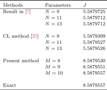
Example 1. Consider the problem [7,25]
minJ = Z 1
0
(x2(t) +u2(t))dt s.t.
˙
x(t) =u(t),
u(t)61,
x(0) = 1 + 3e 2(1−e).
For comparison our method with [25] and [7], we give Table1, in which the optimal performance indices obtained by using our method and those listed in [25] and [7] are shown. In Table1, N is the number of mesh-points for the Chebyshev-Legendre collocation method. In Figure 1, exact and approximated results of the optimal control variable obtained from B-spline functions withM = 8 are reported.
Figure 1. Exact value and approximation of optimal control vari-able using B-spline functions for Example1 withM = 8.
Table 1. Estimated and exact values ofJ for Example1
Methods Parameters J
Result in [7] N= 9 5.5879725
N= 11 5.5879712
N= 13 5.5879712
CL method [25] N= 9 5.5879399
N= 11 5.5879527
N= 13 5.5879526
Present method M= 8 8.5879530
M= 9 8.5879551
M= 10 8.5879557
Exact 8.5879557
Legendre polynomials [15]. Find the control vectoru(t) which minimizes
J= 1 2
Z 1 0
subject to
˙ x1(t)
˙ x2(t)
=
0 1 0 −1
x1(t)
x2(t)
+
0 1
u(t),
x1(0)
x2(0)
=
0 10
,
and subject to the following inequality control constraint
|u(t)|61.
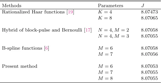
In Table 2, K in [19] is the order of Rationalized Haar functions, and N and M in [17] are the order of block-pulse functions and Bernoulli polynomials, respectively. In Figure 2, the control and state variables with the absolute value of constraint’s errors for two methods of B-spline functions withM = 7, are reported.
Table 2. Results for Example2
Methods Parameters J
Rationalized Haar functions [19] K= 4 8.07473
K= 8 8.07065
Hybrid of block-pulse and Bernoulli [17] N= 4, M= 2 8.07058
N= 4, M= 3 8.07055
B-spline functions [6] M= 6 8.07058
M= 7 8.07056
Present method M= 6 8.07053
M= 7 8.07055
M= 8 8.07055
Example 3. In order to show the effectiveness of the proposed method, the contin-uous stirred-tank chemical reactor as a benchmark problem in the class of nonlinear optimal control problems is considered. This example is adapted from [10]. The state equations of the system are highly nonlinear and coupled:
˙
x1(t) =−2 (x1(t) + 0.25) + (x2(t) + 0.25) exp 25x
1(t)
x1(t) + 2
−(x1(t) + 0.25)u(t),
˙
x2(t) = 0.5−x2(t)−(x2(t) + 0.5) exp 25x
1(t)
x1(t) + 2
.
The initial conditions are
x1(0) = 0.05, x2(0) = 0.
The performance index to be minimized is given by
J= Z 0.78
0
(a) (b)
Figure 2. State and control variables and the constraint errors
|x˙1(t)−x2(t)|and|x˙2(t) +x2(t)−u(t)|for Example2 using present
wherex1(t) is the deviation from the steady-state temperature,x2(t) is the deviation
from the steady-state concentration andu(t) is the normalized control variable that represent the effect of the flow-rate of the cooling fluid on chemical reactor. The performance index indicates that the desired objective is to maintain the temperature and concentration close to their steady-state values without expending large amount of control effort.
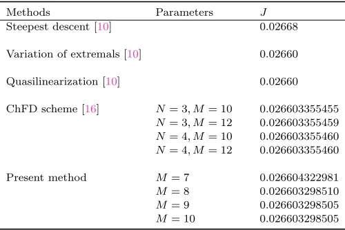
This problem was solved using three different numerical methods: steepest-descent, variation of extremals, and quasilinearization [10]. In Table3, the solutions obtained by the proposed method for different values ofM are compared with existing solutions.
Table 3. Results for Example3
Methods Parameters J
Steepest descent [10] 0.02668
Variation of extremals [10] 0.02660
Quasilinearization [10] 0.02660
ChFD scheme [16] N= 3, M= 10 0.026603355455
N= 3, M= 12 0.026603355459
N= 4, M= 10 0.026603355460
N= 4, M= 12 0.026603355460
Present method M= 7 0.026604322981
M= 8 0.026603298510
M= 9 0.026603298505
M= 10 0.026603298505
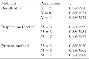
Example 4. The current example is the nonlinear forced Van-DerPol oscillator given in [7,22]. The cost, dynamics, and constraints are the following:
minJ = 1 2
Z 5 0
(x21+x22+u2)dt s.t.
˙
x1(t) =x2(t),
˙
x2(t) =−x1(t) + (1−x1(t))x2(t) +u(t),
x1(0) = 1, x2(0) = 0, x2(5)−x1(5)−1 = 0.
Table 4. Results for Example4
Methods Parameters J
Result of [7] N= 7 0.3807970
N= 9 0.3807971
N= 11 0.3807971
B-spline method [6] M= 5 0.3807999
M= 6 0.3807981
M= 7 0.3807977
Present method M= 5 0.3807970
M= 6 0.3807969
M= 7 0.3807968
6. Conclusion
In this paper we presented a numerical scheme for solving nonlinear constrained quadratic optimal control problems. The method of B-spline functions was employed. Also several test problems were used to see the applicability and efficiency of the method. The obtained results show that the new approach can solve the problem effectively.
References
[1] R. Bellman,Dynamic Programming, Princeton, NJ: Princeton University Press, 1957. [2] R. Bellman, R. Kalaba and B. Kotkin, Polynomial Approximation – A New Computational
Technique in Dynamic Programming: Allocation Processes, Mathematics of Computation,17
(1963), 155–161.
[3] R. E. Bellman and S. E. Dreyfus,Applied Dynamic Programming, Princeton University Press, 1971.
[4] H. B. Curry and I. J. Schoenberg,On Polya frequency functions IV: the fundamental spline functions and their limits, J. Analyse Math.,17(1966), 71–107.
[5] C. De. Boor,A practical guide to spline, Springer–Verlag, New York, 1978.
[6] Y. Edrisi Tabriz and M. Lakestani,Direct solution of nonlinear constrained quadratic optimal control problems, Kybernetika,51(1) (2015), 81–98.
[7] M. El-Kady,A Chebyshev finite difference method for solving a class of optimal control prob-lems, International Journal of Computer Mathematics,80(2003), 883–895.
[8] Z. Foroozandeh and M. Shamsi,Solution of nonlinear optimal control problems by the interpo-lating scaling functions, Acta Astronautica72(2012), 21–26.
[9] J. C. Goswami and A. K. Chan,Fundamentals of wavelets: theory, algorithms, and applications, John Wiley & Sons Inc. 1999.
[10] D. E. Kirk, Optimal Control Theory: An Introduction, Prentice-Hall, Englewood Cliffs, NJ, 1970.
[11] M. Lakestani and M. Dehghan,Numerical solution of generalized Kuramoto-Sivashinsky equa-tion using B-spline funcequa-tions, Applied Mathematical Modelling,36(2012), 605–17.
[12] M. Lakestani, M. Razzaghi and M. Dehghan,Solution of nonlinear FredholmHammerstein inte-gral equations by using semiorthogonal spline wavelets, Mathematical Problems in Engineering,
1(2005), 113–21.
[13] M. Lakestani, M. Dehghan and S. Irandoust-pakchin,The construction of operational matrix of fractional derivatives using B-spline functions, Commun Nonlinear Sci. Numer. Simulat.17
[14] P. Lancaster,Theory of Matrices, Academic Press, New York, 1969.
[15] H. R. Marzban and M. Razzaghi,Hybrid functions approach for linearly constrained quadratic optimal control problems, Appl Math Modell27(2003), 471–85.
[16] H. R. Marzban and S. M. Hoseini,A composite Chebyshev finite difference method for nonlinear optimal control problems, Commun Nonlinear Sci. Numer. Simulat.18(2013), 1347–61. [17] S. Mashayekhi, Y. Ordokhani and M. Razzaghi,Hybrid functions approach for nonlinear
con-strained optimal control problems, Commun Nonlinear Sci. Numer. Simulat.17(2012), 1831–43. [18] R. K. Mehra and R. E. Davis,A generalized gradient method for optimal control problems with
inequality constraints and singular arcs, IEEE Trans. Automat Contr.17(1972), 69–72. [19] Y. Ordokhani and M. Razzaghi,Linear quadratic optimal control problems with inequality
con-straints via rationalized Haar functions, Dyn. Contin. Discrete Impul. Syst. Ser B12 (2005), 761–73.
[20] M. Razzaghi , and G. Elnagar,Linear quadratic optimal control problems via shifted Legendre state parameterization, Internat J. Systems Sci.25(1994), 393–99.
[21] L. L. Schumaker,Spline functions basic theory, Cambridge University Press, New York, 2007. [22] A. Schwartz,Theory and implementation of numerical methods based on Runge-Kutta
integra-tion for solving optimal control problems, A Bell & Howell Information Company, Ann Arbor, MI, 1996. Thesis (Ph.D.)–Berkeley - U.C.
[23] J. Vlassenbroeck and R. Vandooren,A Chebyshev technique for solving nonlinear optimal con-trol problems, IEEE Trans. Autom. Control33(4) (1988), 333–40.
[24] V. Yen and M. Nagurka,Linear quadratic optimal control via Fourier-based state parametriza-tion, J. Dyn. Syst. Meas. Control113(2) (1991), 206–15.
![Figure 2. State and control variables and the constraint errorsmethod (a) and using method of [| ˙x1(t) − x2(t)| and | ˙x2(t) + x2(t) − u(t)| for Example 2 using present6], (b) with M = 7.](https://thumb-us.123doks.com/thumbv2/123dok_us/8943957.1853325/10.612.126.476.108.600/figure-control-variables-constraint-errorsmethod-method-example-present.webp)