*Corresponding Author: [Mohamed A.E. AbdelRahman]. (E-mail: [email protected]).
DOI :10.21608/ejss.2017.255.1043
A
GRICULTURAL Land use planning is mainly attributed to the area of each class of soil capability and its suitability degree for the different land use types. This study was conducted to examine the areas of land evaluation (LE) that could be determined based on two approaches; first based on the geomorphological mapping units which were elaborated from remotely sensed data and second based on the spatial distribution of land evaluations parameters using geostatistical techniques (Universal Kriging) in North Delta, Egypt. The objective of this study was to evaluate the available land resources and produce land evaluations maps using geostatistical and physiographic methods. Sixty soil profiles were collected to represent the different mapping units and analyzed for land evaluation assessment. The LE of the study area was classified into C1, C2, C3, and C4 for land capability and was classified into S1, S2, S3 and N1 for land suitability by adopting the logical criteria. The result demonstrates that the study area can be categorized into spatially distributed LE based on soil characteristics and analyzing present land use using geostatistical as well as physiographic units. The obtained results are considered useful tools for guiding policy decision makers for the sustainable management of land resources in the investigated area.Keywords: Land capability, Geostatistics, Land evaluation, Physiography mapping units, Spatial modeling, Remote sensing.
Introduction
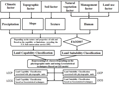
Land evaluation (LE) for agriculture use is a process needing specialized geo-environmental information and a scientist expertised in computer to analyze and interpret the information. According to FAO (2007) land evaluation (LE) is defined as assessment of land performance used for specified purposes. LE determining basically depends on surveys of climate, soils, vegetation and other aspects of land in terms of the requirements of alternative forms of land use. LE in this study is concerned with comparing the representation of LE classes based on referring the soil characteristics to the geomorphological units which were based for collection of the soil profiles, and generating the spatial distribution of LE limitation factors using geostatistical technique. This study will show the difference between using the weighted average of the represented soil profile values for the geomorphology unit and using all values of
each soil profile for the same geomorphology unit. The result will provide a reason for accepting the two methods undifferentiated. This study involves how much change and its effects with change in the method used of representing LE and change in the every class area itself.Modeling the spatial depended of fecal coliform with a semivariogram. The lag size was controlled for grouping samples for better spatial correlation in the data. The variogram was produced and clearly showed increasing semivariance with increasing separation distance. This was done to produce a better model as modeling the semivariance is an iterative process. The importance of this study is lying on the area of LE classes and their degrees helping in choosing suitable uses of land which are physically possible and economically and socially relevant. Also, determining the levels of soil improvements and management practices could be implemented offering possibilities of sustained production. GIS is helpful for processing large
A GIS Based Model for Land Evaluation Mapping: A Case Study
North Delta Egypt
A. Shalaby 1, M.A.E. AbdelRahman 1*, A. A. Belal 2
1Division of Environmental Studies and Land Use and 2Agriculture Applications,
amounts of spatial data and providing accurate and accessible information for land (Arnous and Hassan, 2006).
The processing of LE using Geostatistic techniques supports the production of thematic maps. Building GIS database is helping in outlining limiting factors, accordingly suggestions for sustainable agricultural use (Ali et al., 2007). Land capability is the inherent physical capacity of the land to sustain a range of land uses and management practices in the long term without degradation to soil, land, air and water resources (Central West CMA, 2008, Dent et al., 1981, Rowe et al., 1981 and Sonteret al., 2007). According to Lawrie et al. (2007) Failure to manage land in accordance with its capability risks degradation of resources both on- and off-site, leading to a decline in natural ecosystem values, agricultural productivity and infrastructure functionality. Remote Sensing and GIS spatial modeling is a useful tool in generating spatial and quantitative information on land status of any area and for thematic mapping (AbdelRahman et al., 2015 a,b). Land suitability is the ability of soil to produce crops in a sustainable way. Identifyingthe limiting factors for the agricultural production enables decision makers to develop crop managements which are reflected in
increasing the land productivity. The objective of this study was to develop a GIS based approach for LE assessment which will assist decision makers. Also, determining LE classes is useful to identify the management requirements to ensure sustainable agricultural use without causing a significant on-site or off-site degradation to land quality.
Materials and Methods
Study area
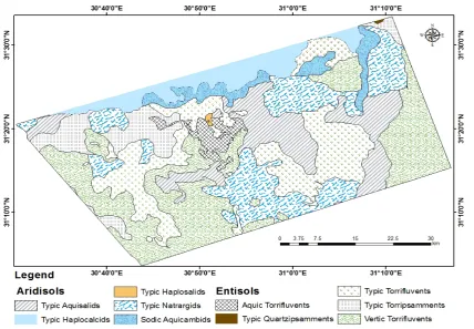
The study area is located in the northern tip of Nile Delta; with an area about 2260 Km2 (Fig. 1, showing profiles locations as well) it extended between North latitudes 31o 3’12’’ to 31o 33’27’’ and East longitudes 30o 30’31’’ to 31o 16’42’’. It falls in the semi-arid zone.
Georeferenced Soil survey data, field work observations and laboratory analysis of the profiles samples (Fig. 1) have been integrated in a GIS based LE assessment (FAO, 2007) for agricultural use in the study area. LE maps for soil suitability and capability were developed based on geomorphology units and Geostatistics techniques to illustrate LE categories and display the spatial representation of each category for agriculture.
Methods of soil analysis
Soil samples upon arrival in the laboratory were air dried under shade and then crushed in a wooden mortar with a pestle and sieved through a 2 mm sieve to separate the coarse fragments (> 2mm). The fine earth was stored in separate containers and used for analysis.
Physical characteristics
The international pipette method was used for particle size analysis as described by Piper (1966).Particle density of the coarse fragments were calculated by taking the ratio of oven dry weight of the coarse fragments to volume of coarse fragments, which was obtained through water displacement method.
Chemical characteristics
The soil reaction (pH) was determined in 1: 2.5 soil : water suspension by potentiometric method using glass electrode (Jackson, 1973). Electrical conductivity (EC) of the saturated soil water extract was measured using Elico conductivity bridge (Model CM 82 T) (Jackson, 1973).The cation exchange capacity of soils was determined by leaching the soil with sodium acetate buffered to 8.5 and then replacing sodium from sodium saturated soils with ammonium by leaching with ammonium acetate. The exchangeable sodium in the leachate was determined by flame photometer model Elico and values were expressed as cmol (P+) kg-1 soil (Baruah and Barthakur, 1999).The organic carbon was estimated by Walkley and Black wet-oxidation method (Jackson, 1958). To overcome the effect of excessive soluble chloride in these soils, silver sulphate was added to sulphuric acid (USSL Staff, 1954). Available nitrogen content of the soil was determined by following alkaline potassium permanganate method (Subbaiah and Asija, 1956). In the available phosphorus determination, extraction was done by using Olsens’sextractant (0.5 N Sodium bicarbonate; pH 8.5) as all the soils are calcareous except pedon 11, which is noncalcareous and extraction was done using Bray and Kurtz No 1 extractant. Phosphorus in the extract was estimated by developing blue colour with ammonium molybdate using ascorbic acid as reductant. Colour intensity was measured at 660 nm in Spectro-photometer (Jackson, 1973). In the available potassium determination, extraction was done by neutral normal ammonium acetate and subsequent estimation by atomic absorption spectrophotometer (Jackson, 1973). Cationic micronutrients such as iron, copper, manganese and zinc were extracted by DTPA extract (0.005 M
diethylene triaminepenta acetic acid and 0.01 M CaCl2 + 0.1 N triethanolamine at pH 7.3) and the concentration was measured in atomic absorption spectrophotometer as outlined by Jackson (1973). The exchangeable cations like sodium and potassium were extracted with 1N ammonium acetate as described by Baruah and Barthakur (1999). The procedure followed for estimation of sodium and potassium was similar to those outlined for water soluble cations in calcareous soils. But cations like calcium and magnesium were extracted with 1 N KCl + TEA extractant and analysed with AAS. (Sarma et al., 1987).
Physiography and soils mapping
By extracting rasterized geomorphologic units, victorizing then geomorphologic units were obtained using Arc GIS 10.1. The main criteria for delineating land types is the physiographic analysis as proposed by Burnigh (1960) and Goosen (1967). The goal of this method is to identify boundaries, correlated to differences in physiographic processes. This method is called the “genitic approach”, which is based on the dynamic processes rather than the static ones.The spectral signatures of bands were used as a composite output for the purpose of visual analysis. This method
is of benefit especially when focusing on the infrared
bands that permit the detection and discrimination of broad combinations of different vegetation cover
types and identification of water bodies, active
drainage, drainage conditions cultivated areas, and bare areas. This land sat image is considered as a source of much more recent information that can
be aimed for transfering the recent or modified
infrastructures to the maps during the phase of cartography.
taxonomy (USDA, 2014) was used to classify the different soil profiles to subgroup level, and then the correlation between the physiographic and taxonomic units was designed (Elbersen et al., 1986).The landforms (Fig. 3) were delineated by overlapping the digital elevation model with Landsat and verified using ground truth data during the soil profiles collection processes. Then representing landforms was considered as a base map for producing soil map of the studied area (Fig. 4).
According to Shatta (1984), the Nile Delta is a plain gently sloping in much of the northern half of the Delta, the gently sloping northwards was occupied in the northern portion extensive wet land and salt marches and characterized by relief and bounded on the south by a moderately elevated. Bayoumy (1992) stated that the relief showed to be a main factor in the differentiation of soil properties and grouping. Accordingly, salinity and ground water table are changing.
Geostatistical technique
Geostatistical (Universal Kriging approach) in Arc-GIS 10.1 software has been used for interpolating soil properties, mapping and producing
LE maps. Geostatistical is based on an assumption that things close to one another are more alike than those which are farther apart. Minimizing root mean square prediction error (RMSPE) was used to determine the optimal power value. Modelsin kriging were fitted using the variogram. Variogram showed increasing semivariance with increasing separation distance which means fitting the lag size produced a better model. There are three major properties characterizing the variogram known as nugget effect, sill and range. Nugget effect is the discontinuity of the variogram which expresses both variability at a scale smaller than the sampling interval and non-spatial variation. Repeated measurements is the only way to remove the nugget effect which cannot be removed by close sampling (Trangmar et al., 1985). Range is lag distance sill expresses distance for uncorrelated samples. After knowing variogram , prediction of mapping unit can be done from the available data points using kriging. Standard deviation of prediction error given by Kriging depends only on the variogram, the number of data and the spatial configuration with which these are taken (Burrough, 1991). Geostatistical analyses were performed using the Geostatistical analyst extension available in ESRI ArcMap v 10.2(ESRI 2012).
Fig. 3. Land forms of the study area, after Darwish and Abdel Kawy, 2008
Land evaluation assessment
Land capability classification was also undertaken based on the capability or limitations according to the U. S. Soil conservation service (1992). While Land evaluation classification was undertaken according to the FAO (2007) system to assess the suitability of the studied area soils for agriculture and development. A set of 60 soil profiles collected and soil samples were analyzed for pH, EC, BD, SAR, CEC, CaCO3, ESP, Gypsum, Available macronutrients, micronutrients, Irrigation water type, profile depth, water table depth, texture, and SOC content, All parameters were initially included in LE model as shown in Fig. 2.
Results
Physiographic
The study area was classified to three landscape units (Flood plain, Lacustrine plain, and Marine plain) and into sixteen land form units (Decantation basins, Dried fish ponds, Dried lake bed, Island, Isolated hills, Overflow basins, Overflow mantle, High river terraces, Moderately high river terraces, Low river terraces, High elevated sand sheet, Sand sheet (High elevated, Shifting sand dune), Sand sheet (Low elevated), Seasonally submerged land, Water bodies, and Wetlands). The terraces in the study area which are landform level divided into three relief level ; low, moderately high river terraces for better distribution of the profiles locations to reach the target of quantitative and qualitative comparison in this study.
Irrigation water
Fresh and blended water are used for agricultural irrigation in the area. pH of fresh irrigation water in the area ranged from 7.2 to 7.5,EC ranged from 0.6 to 0.9 dS/m and SAR ranged from 2.2 to 2.4 while for blended water 7.6 to 8.2 for and EC ranged from 1.6 to 3.4 dS/m and SAR ranged from 3.8 to 7.9.
Soil
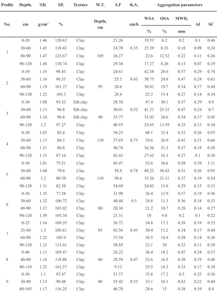
Sixty soil profiles were digged and collected. Soil samples were analyzed for their physio-chemicals properties and some representative analyses are presented in Tables 1 and 2 the results were used in producing soil map, suitability and capability results.
In this study, a soil map was produced based on analyzing and description in details of site, morphological characteristics, physical and chemical properties of collected Pedon’s samples from soils of the investigated area.Soil of the study area was classified as shown in Fig. 4 according to soil taxonomy, (Soil Survey Staff., 2014) to two orders; Aridisols, Entisols and to ten sub great groups units; (Typic Aquisalids Salitorrerts, Aquic Torrifluvents, Sodic Aquicambids, Typic Aquisalids, Typic Haplocalcids, Typic Haplosalids, Typic Natrargids, Typic Quartzipsamments, Typic Torrifluvents, Typic Torripsamments, Vertic Torrifluvents) as shown in Fig. 2.
Land Capability Classification (LCC)
Classification of soils based on land capability helps in estimating soil resources available for different purposes and for appropriate use of soils without deterioration. The recorded largest LC in the area is for C3 with total area ranged between 806.8 to 895.8 km2 when the smallest belongs to C1 with total area ranged between 73.5 to 73.8 Km2.The areas for each single class is different based on the methodology used for representation of the spatial distribution.
From Table 1 the results showed that C1 is having and equal percent of both areas using the two representative methods while C2 showed a slight difference in both areas and the difference in areas increased in C4 classes while the largest difference is in C3 classes based on the two methods used for the representation of each class. The percentages of each class and areas based on the two methodologies are shown in Table 3 and Fig. 5 & 6.This result may be due to the locations of profiles which were selected to represent the physiographic mapping units designed based on a semi grid sampling system. So, High correlation between the two methods is expected as the same samples used. The profile locations are fairly dense and uniformly distributed throughout the study area;this may be the main cause of fairly good estimation results regardless of interpolation algorithm, Kriging is used to spatially determine the total amount of the variables over the region instead of the continuous distribution of those variables over geomorphology. For this reason the error maps were not presented as a result of controlling the lag size for grouping samples for better spatial correlation in the data.
TABLE 1. Soil analyses of some representative profiles
Profile Depth, ΒD, SP, Texture W.T. S.F K.S, Aggregation parameters
No. cm g/cm3 % Depth,
cm cm/h
WSA OSA MWD,
AI SC
% % mm
1
0-30 1.46 120.63 Clay 21.26 19.53 6.2 0.2 0.1 0.46
30-60 1.45 118.43 Clay 24.78 0.35 25.39 8.33 0.18 0.09 0.24
60-90 1.47 123.67 Clay 105 26.27 22.6 12.52 0.22 0.11 0.26
90-120 1.48 130.74 Clay 29.38 17.27 8.26 0.13 0.07 0.29
2
0-30 1.16 98.43 Clay 24.61 42.38 28.6 0.57 0.29 0.74
30-60 1.16 96.35 Clay 25.3 0.43 38.75 24.8 0.47 0.24 0.63
60-90 1.19 101.37 Clay 95 28.6 30.41 19.7 0.34 0.17 0.44
90-120 1.22 105.3 Clay 28.4 25.3 15.4 0.27 0.14 0.34
3
0-30 1.08 93.33 Silt clay 28.58 47.4 30.1 0.57 0.29 0.9
30-60 1.13 96.8 Silt clay 30.01 0.52 41.21 25.31 0.47 0.24 0.7
60-90 1.16 96.8 Silt clay 90 35.77 31.02 20.6 0.34 0.17 0.45
90-120 1.2 97.27 Clay 40.55 25.65 13.59 0.25 0.13 0.34
4
0-30 1.03 82.4 Clay 36.23 48.1 32.4 0.52 0.26 0.93
30-60 1.13 84.3 Clay 110 37.65 0.75 39.6 26.9 0.41 0.21 0.66
60-90 1.21 86.8 Clay 40.76 36.56 21.3 0.37 0.19 0.58
90-120 1.15 87.16 Clay 42.43 27.62 16.3 0.27 0.1 0.38
5
0-30 1.01 75.51 Clay 45.47 52.6 36.6 0.58 0.29 1.11
30-60 1.04 79.6 Clay 54.8 0.78 48.23 30.43 0.51 0.26 0.93
60-90 1.2 80.39 Clay 110 50.6 35.26 21.11 0.37 0.19 0.54
90-120 1.11 82.38 Clay 54.69 24.83 15.8 0.29 0.15 0.33
6
0-30 1.35 77.58 Clay 31.98 26.4 13.9 0.37 0.19 0.36
30-60 1.32 106.72 Clay 40.48 0.3 24.8 11.3 0.36 0.18 0.33
60-90 1.37 103.02 Clay 80 20.36 21.2 10.7 0.28 0.14 0.27
90-120 1.39 103.34 Clay 21.31 18 9.8 0.2 0.1 0.22
7
0-25 1.16 109.35 Clay 36.72 34.6 17.1 0.38 0.19 0.53
25-60 1.2 105.61 Clay 85 42.56 0.45 30.4 15.2 0.34 0.17 0.44
60-90 1.22 105.9 Clay 33.54 26.5 14.4 0.28 0.14 0.36
90-120 1.23 131.41 Clay 58.85 22.1 10 0.22 0.11 0.28
8
0-40 1.13 105.47 Clay 26.22 36.4 18.2 0.47 0.24 0.57
40-80 1.16 118.88 Clay 80 28.59 0.47 32.6 16.5 0.38 0.19 0.48
80-110 1.23 161.57 Clay 9.12 25.5 14.3 0.33 0.17 0.34
9
0-30 1.1 92.47 Clay 51.57 35.8 17.2 0.5 0.25 0.56
30-80 1.15 90.48 Clay 80 55.42 0.52 33.1 16.1 0.43 0.22 0.44
80-105 1.17 116.25 Clay 46.78 28.6 15 0.38 0.19 0.4
TABLE 2. Soil analyses of some representative profiles
Profile Depth, pH EC, OM SAR CEC CaCO3 ESP Gyp.
No. cm 01:02.5 dS/m % cmol/kg % % %
1
0-30 8.07 50.3 0.59 45.88 31.4 1.76 43.69 0.2
30-60 8.1 46.3 0.5 44.26 23.8 2.44 54.11 0.2
60-90 8.16 54.6 0.4 47.76 22.2 2.44 67.56 0.2
90-120 8.29 60 0.3 48.4 23.8 2.66 60.33 0.2
2
0-30 7.9 7.1 1.18 12.6 29.2 1.33 23.86 0.2
30-60 8.11 7.9 1.07 15.1 27.6 1.44 34.56 0.3
60-90 8.2 8.2 0.9 16.19 32 1.89 23.81 0.3
90-120 8.17 8.6 0.7 17.18 26.8 1.89 48.2 0.4
3
0-30 7.98 6.15 1.86 12.12 33.6 0.98 21.51 0.4
30-60 8.1 6.8 0.7 12.52 35.2 1.88 25.48 0.1
60-90 7.99 7.2 15.1 28.4 1.88 38.13 0.2
90-120 8.13 7.9 16.7 34.4 1.66 36.16 0.5
4
0-30 7.99 6 2.24 11.19 37 0.88 13.73 0.4
30-60 8.13 6.4 0.78 11.72 35.2 1.32 16.42 0.2
60-90 8.01 7.1 0.7 12.22 32.8 1.9 20.33 0.2
90-120 7.95 7.8 0.3 13.72 28.4 1.1 24.6 0.4
5
0-30 7.66 3.1 1.87 10.35 38 0.33 12.1 0.6
30-60 7.81 5.3 1.62 12.14 36.2 1.44 14.5 0.4
60-90 7.98 7.5 1.07 13.98 32 1.89 16 0.1
90-120 8.1 7.6 0.55 14.86 28.4 1.94 25.47 0.5
6
0-30 8.2 46.2 1.34 40.33 22 1.64 50.7 0.3
30-60 8.23 42.75 0.88 43.88 23 2.32 62.28 0.3
60-90 8.25 40.31 0.55 41.14 22.4 2.21 48.35 0.3
90-120 8.3 37.94 0.3 39 21.6 3.21 65.51 0.3
7
0-25 8.1 8.3 1.48 15.08 25.2 1.08 28.17 0.4
25-60 8.15 8.8 1.09 16.16 22.4 1.7 37.72 0.4
60-90 8.2 9.5 0.7 17.02 20 1.32 49.6 0.4
90-120 8.3 11.8 0.5 18.53 21 3.9 32.95 0.4
8
0-40 8.12 7.8 1.83 13.99 30.2 2.42 22.12 0.4
40-80 8.15 8.7 0.9 15.6 23.6 1.98 35.88 0.4
80-110 8.25 10.2 0.3 16.8 19.1 0.44 39.58 0.4
9
0-30 7.82 7.2 1.7 14.29 22.4 2.55 18.86 0.3
30-80 8.11 8.4 1.1 15.1 26 0.88 22.42 0.3
TABLE 3. Area of land capability classes
Land Capability Classes LCCP area LCCG area
% Km2 % Km2
C1 3.3 73.5 3.3 73.8
C2 20.7 468.2 20.0 452.2
C3 35.7 806.8 39.6 895.8
C4 33.7 762.7 30.5 688.7
Island 0.1 2.5 0.1 2.4
Water bodies 6.5 146.4 6.5 146.4
% of the total area, LCC is land capability classification, LCCP is based on physiographic units, and LCCG is based on Geostatistical technique.
Fig. 5.Spatial distribution of LCCG Fig. 6. Spatial distribution of LCCP LCC is land capability classification, LCCG is based on Geostatistical technique, and.LCCP is based on physiographic units.
According to FAO (2007), soils of the study area could be classified as shown in Table 4 and Fig. 7 and 8 into four classes recognized within two orders (S for suitable and N for not suitable) and according to this system Land Suitability units were represented based on association with physiographic units and based on kriging geostatistical approach and were identified as shown in Table 2 and Fig 7 & 8 , respectively. From
TABLE 4. Area of land Suitability classes.
Land Suitability Classes
LSCP area LSCG area
% Km2 % Km2
S1 3.3 73.5 5.4 121.7
S2 20.7 468.2 21.2 478.2
S3 67.6 1527.6 65.6 1483.6
N1 1.9 41.9 1.2 27.5
Island 0.1 2.5 0.1 2.5
Water bodies 6.5 146.4 6.5 146.4
% of the total area, LSC is land suitability classification, LSCP is based on physiographic units, and LSCG is based on Geostatistical technique.
Table 2 the representations methods showed a slight difference between same class in each methods.
Fig.7. Spatial distribution of LSCG Fig. 8. Spatial distribution of LSCP
LSC is land suitability classification, LSCP is based on physiographic units, and LSCG is based on Geostatistical technique.
Results showed that land units which have no limitations cover about 3.3 % which association with physiographic units and for those representing based on Geostatistic technique cover about 5.4% of the study area. Total area of land units that are marginally suitable for agriculture is around 65.6 (LSCG) to 67.6 % (LSCP) of the study area. The study showed also that GIS based approach is a useful tool in land suitability assessment for agricultural planning.
Statistical correlations between the different methods used
The results in this study were statically compared using the correlation between LSCP and LSCG and the correlation between LCCP and LCCG. The result R2 = 0.96 indicated that LSCP and LSCG calculations having high significant correlations in both methods used (representing spatial distribution of LSC associated with the
Fig. 9. Statistical correlation between LSCP and LSCG and between LCCP and LCCG based on Physiographic and Geostatistical approach
physiographic units or using kriging Geostatistical approach) as shown in Fig. 9.
Also, the result R2 = 0.93 indicated that LCCP and LCCG calculations having high significant correlations in both methods used (representing spatial distribution of LCC based on physiographic units or using Geostatistical approach) as shown in Fig. 9.
Discussion
Kriging was tested by Van Kullenburg et al. (1982), Shalaby et al. (2006), AbdelRahman (2008,2009,2014) and AbdelRahman et al. 2015 a,b). They stated that Kriging is the best among spatial interpolation techniques namely; Proximal, weighted average and Kriging. Also, they mentioned that difference in accuracy between Kriging and the relatively simple weighted average technique could be neglected in practice. This study stated that kriging method was the suitable technique for the spatial representations of LCC and LSC in the selected area , also it is in agreement with AbdelRahman (2014).
The overall results showed a slight difference in terms of the representative class and its total area. This led to the recommendation of using the geostatistical method and Arc GIS model builder to produce the the matic maps based on well distributed sits of profiles samples. Although the geomorphology based method is still effective in the areas with different topography.
Conclusion
For determining the LC and LS maps, the different parameters such as pH, EC, BD, SAR, CEC, CaCO3, ESP, Gypsum, Available macronutrients, micronutrients, irrigation water type, profile depth, Water table depth, texture, and SOC content were used. After generating the interpolation maps with the Inverse Distance Weighted (IDW), the fuzzy maps were generated by the membership functions for each parameter.The output from an evaluation normally gives information on potential form of use for each area of land, including the consequences, beneficial and adverse, of class degree. Such kind of LCC and LSC analyses allows identifying the main limiting factors for the agricultural production and enables decision makers to develop crop managements practices which may be able to increase the land productivity. The methods used for representing evaluation process determine the area of each soil class, and provide data on the basis of which such decisions can be taken. Spatial interpolation and kriging effective in this role should be from well distributed even based soil samples.
References
AbdelRahman, M. A. E., Natarajan A. and Hegde, R. (2015 a) Climate and its impact on soil biological degradation using GIS and remote sensing (I): Biological degradation as a result of deterioration of organic matter by climate. J. Soil Biol. Ecol.,35 (1& 2),192-201, 2015
AbdelRahman, M. A. E., Natarajan, A. and Hegde R. (2015 b) Climate and its impact on soil biological degradation using GIS and remote sensing (II): Biological degradation as a result of removing organic matter by water erosion. J. Soil Biol. Ecol., 35 (1&2), 208-216, 2015
AbdelRahman, M.A.E. et al. (2016a) Estimating soil fertility status in physically degraded land using GIS and remote sensing techniques in Chamarajanagar district, Karnataka, India. Egypt. J. Remote Sensing Space Sci.,http://dx.doi.org/10.1016/j.ejrs. 2015.12.002
AbdelRahman, M.A.E. (2016b) Assessment of land suitability and capability by integrating remote sensing and GIS for agriculture in Chamarajanagar district, Karnataka, India, Egypt. J. Remote Sensing Space Sci.,http://dx.doi.org/10.1016/j. ejrs.2016.02.001
AdelRahman, M. A. E. (2009) Quantification of Land Degradation Indicators Using Remote Sensing and GIS Techniques. M. Sc. Thesis submitted to Zagazig University, Egypt.
AdelRahman, M. A. E. (2014) Assessment of Land Degradation and Land Use Planning by Using Remote Sensing and GIS Techniques in Chamarajanagar District, Karnataka Ph.D. Thesis submitted to UAS, Bangalore University, India. AdelRahman, M. A. E., Tahoun, S.A., Abdel Bary,
E. A. and Arafat, S. M. (2008) Detection land degradation processes using geostatistical approach in Portsaid, Egypt. Zagazig J. Agric. Res.,35 (6) 2008,1361-1379.
Arnous, M.O. and Hassan, M.A.A. (2006) Image processing and land information system for soil assessment of El-Maghara Area, North Sinai, Egypt. In: International Conf. on Water Resources and Arid Environment.
(1992) Mineralogical study of soils belonging to different physiographic units in the eastern side of Egypt. Egypt. J. Soil Sci. 32, (3), pp. 437-453.
Burnigh, P. (1960) The applications of aerial phothographs in soil surveys, Man. of Photogr. Interpr., Washington, D.C., U.S.A, pp. 633-666.
Burrough P. A. (1991) “Sampling Designs for Quantifying Map Unit Composition,” In: M. J. Mausbach and L.P. Wilding, (Ed.), Spatial Variabilities of Soils and Landforms, SSSA Spec. Publ. 28, SSSA, Madison.
Central West CMA (2008) Land and Soil Capability – How we safely manage the land. Land classifications of the Central West – 2008. Central West Catchment Management Authority, Wellington, NSW.
Darwish Kh. M. and Abdel Kawy W.A. (2008) Quantitative assessment of soil degradation in some areas North Nile Delta, Egypt. Int J Geol 2(2):17–22.
Elbersen, G.W.W and R. Catalan (1986) Portable computer in physiographic soil survey. Proc. Intemat Soil Sci., Cong.Homburg.
ESRI (2012) “ArcMap Version 10.2 User Manual,” Redlands.
FAO (2007) A Framework for land evaluation (Land evaluation, Towards a revised framework) FAO Soil Bulletin No. 6 Rome. Italy.
FAO (2006) Guidelines for Soil Description, Fourth edition. Food and Agriculture Organization of the United Nations Rome, ISBN 92-5-105521-1 Goosen, D. (1967) Aerial photo interpretation in
soil survey. FAO Soil Bull. No. 6, FAO, Rome, Italy.
Lawrie, J., Murphy, B., Packer, I.J. and Harte, A.J. (2007) Soils and Sustainable Farming Systems, in Soils: Their Properties and Management, 3rd edition, PEV Charman and BW Murphy (Ed.). Oxford University Press, Melbourne.
R.R. Ali, Ageeb, G.W. M.A. Wahab (2007) Assessment of soil capability for agricultural use in some areas west of the Nile Delta, Egypt: an application study using spatial analyses. J. Appl. Sci. Res.3 (11), pp. 1622–1629.
Rowe, R.K., Howe, D.F. and Alley, N.F. (1981) Guidelines for Land Capability Assessment in Victoria. Soil Conservation Authority, Melbourne. Dent, D. and Young, A. (1981) Soil Survey and Land
Evaluation. George Allen & Unwin, London. Shatta, A.A. (1984) Chemical and mineralogical
aspects as a criteria of soil genesis and formation of the region east of the Nile delta. Ph. D. Thesis, Fac. Agric., Zagazig Univ. , Egypt.
SOIL CONSERVATION SERVICE (1992) Washington, DC: Soil Conservation Service, pp. 60-73.
Sonter, R.O. and Lawrie, J.W. (2007) Soils and Rural Land Capability, in Soils: Their Properties and Management, 3rd edition, PEV Charman and BW Murphy (Ed.). Oxford University Press, Melbourne. Trangmar, B.B., Yost, R.S. and Uehara, G. (1985)
“Application of Geostatistics to Spatial Studies of Soil Properties,” In: N. C. Brady (Ed.) Advances in Agronomy, Academic Press Inc., Orlando, Vol. 38, , pp. 45-94.
USDA (2004) Soil Survey Laboratory Methods Manual, Soil Survey Investigation Report No. 42 Version 4.0 November 2004.
USDA Soil Survey Staff. (2014) Keys to Soil Taxonomy, 12th ed. USDA-Natural Resources Conservation Service, Washington, DC.
Zinck, J.A. and Valenzuela, C.R. (1990) Soil geographic database: Structure and Application Examples ITC J., 3, pp. 270–272.
اتلد لامش ىف ةسارد :يضارلأا مييقت طئارخ جاتنلإ ةيفارغجلا تامولعملا مظن مادختسإ
.رصم
للاب زيزعلادبع و ىبلش لداع ، نمحرلادبع دمحم
ءاضفلا مولعو دعب نم راعشتسلإل ةيموقلا ةئيهلا