COST OPTIMIZATION OF ALLOCATING VIRTUAL NETWORK FUNCTIONS WITH PRECEDENCE IN MULTICAST NETWORKS

Creative Components Iowa State University Capstones, Theses and _{Dissertations}

Spring 2019

COST OPTIMIZATION OF ALLOCATING VIRTUAL NETWORK

COST OPTIMIZATION OF ALLOCATING VIRTUAL NETWORK

FUNCTIONS WITH PRECEDENCE IN MULTICAST NETWORKS

FUNCTIONS WITH PRECEDENCE IN MULTICAST NETWORKS

Iowa State University, [email protected]

Follow this and additional works at: https://lib.dr.iastate.edu/creativecomponents

Part of the Digital Communications and Networking Commons

Recommended Citation Recommended Citation

Chalamalasetty, Ramcharan, "COST OPTIMIZATION OF ALLOCATING VIRTUAL NETWORK FUNCTIONS WITH PRECEDENCE IN MULTICAST NETWORKS" (2019). Creative Components. 150.

https://lib.dr.iastate.edu/creativecomponents/150

COST OPTIMIZATION OF

ALLOCATING VIRTUAL NETWORK

FUNCTIONS WITH PRECEDENCE IN

MULTICAST NETWORKS

Creative Component

Master of Science, Computer Engineering

Iowa State University

By

Ramcharan Chalamalasetty

Major Professor

Abstract

In the past few years, Network Function Virtualization (NFV) has been widely

used to reduce the operational and capital costs of implementing network functions

with better performance and easier network management. NFV is a network

ar-chitecture completely built relying on Virtual Network Functions (VNFs). Quite

a few developments have been done for the optimization of resource allocation to

implement VNFs in various networks. In this report, an algorithm for reducing the

cost of placing the VNFs within a Multicast network along with a choice of selecting

the precedence of the VNFs is presented. The proposed approach is formulated as

a Mixed Integer Linear Programming (MILP) model based on a main objective of

minimizing the cost of resource allocation with Precedence in Multicast Networks.

Finally, we evaluate the algorithm through simulations in CPLEX and demonstrate

the results.

Contents

1. Introduction 6

2. Related Work 8

3. Problem and its Formulation 10

The Unicast Problem . . . 10

Objective Function . . . 12

Constraints . . . 12

4. Multicast Algorithm 15

Objective Function: . . . 15

Constraints . . . 17

5. Implementation and Results 21

Unicast Model . . . 21

Multicast Model . . . 23

NSF Network Model . . . 29

6. Conclusion 33

List of Figures

1 Unicast Network . . . 23

2 Unicast Results with No Precedence between VNFs . . . 24

3 Unicast Results with VNF Precedence . . . 25

4 Unicast Results without VNFs . . . 26

5 Multicast Network . . . 27

6 Multicast Results with No Precedence between VNFs . . . 28

7 Multicast Results with Precedence between VNFs . . . 28

8 Multicast Results with No VNFs . . . 29

9 NSF Network . . . 30

10 NSF Network Model Results with No Precedence between VNfs . . . 31

11 NSF Network Model Results with Precedence between VNfs . . . 31

List of Tables

1 Definitions of Parameters and Variables for a Unicast Network . . . . 11

1. Introduction

Multicasting is a process of communicating from a single source to multiple

des-tinations with each destination defined to have its own need. This has become

an emerging service mock that is used by many applications because of its

advan-tages across various networks. Let us consider a Mobile Service Provider (MSP) as

an example. There are various mobiles that support 4G/LTE cellular networks or

some other devices that only support 3G networks. Based on the requirement of

the destination device, the MSP has to configure the networks. So technically the

MSP has to send higher bandwidth signals from Source which can be split using

many types as per the customer’s usage. One more example would be TVs. Some

TVs support 4K UHD signals, while others might support SD signals,etc. In order

to handle all such requests from the destinations and fulfill them at a faster rate,

Multicast communication has been very effective when compared to that of Unicast

communication which happens from one source to one destination.

Nowadays, most of these multicast services are implemented using Network

Func-tions (NFs). Examples of NFs can be load balancers, firewalls, intrusion detection

systems, routers, etc. Many of the Service Providers (SP) currently use several

combinations of NFs to provide the services based on the functionality they wish to

achieve. These NFs are generally implemented using physical devices exclusively

de-signed for the NF’s purpose and these devices are connected to each other to satisfy

the service requirement. The deployment and management of NFs on the physical

devices have become very costly. So, with the main objective of reducing the capital

costs and the operational costs [1], Network Funtion Virtualisation (NFV) has been

proposed by ETSI (European Telecommunications Standards Institute) [2].

NFV is a technique to virtualize the NFs. In other words, it is a process of

as to be operated with efficient management, better performance and lower costs

[1]. These kind of NFs, which can be deployed on NFV infrastructure are known to

be as Virtualised Network Functions (VNFs) [3]. These VNFs can be cascaded and

can also be combined for providing the needed services at reduced operational and

investment costs.

The main aim of this report is to design an optimal routing and VNF placement

algorithm for the virtual networks that support multicasting topology, where the

optimality criterion is to minimize capital and operational costs. In order to meet

specific demands for each destination in a multicast topology, the order of VNFs

in which they will be deployed is also important. The algorithm that we propose

in this report has the ability to place the VNFs as per the destination needs. To

evaluate the proposed algorithm, we have used CPLEX as the optimization solver

of our MILP model.

Remaining chapters of the report are organized as follows. Chapter 2 provides

a review of the literature related to NFV and resource allocation in multicast

net-works. Chapter 3 describes the problem formulation for a Unicast model. Then

in Chapter 4, we show the generalization and development of formulation from a

Unicast model to a Multicast model. Chapter 5 presents simulation models and

the various implementations using those models along with the obtained results.

Finally, a ’Conclusion’ Chapter that discusses about what we have achieved from

2. Related Work

Multicast services involving NFV components (like VNFs) are being widely used

by many applications because of the advantages that we discussed in the previous

chapter. So the need of development in this field has grown a lot. There is a

huge amount of work that has been currently going on across the improvements of

various techniques of to implement NFV for lower network expenditures and better

maintenance. In this chapter, we present some of the works that have helped us

to understand NFV and multicasting. We also discuss some of the techniques that

we included for the solution approach which were already presented across different

papers.

The work presented in [4] explains NFV’s relationships with Software Defined

Networks (SDNs) and cloud computing, etc. So as to have a better understanding

of NFV and the key research areas in the field of NFV, this paper acts as a good

reference which also shows the architecture of NFV as well as state-of-the-art survey

on NFV. However, this paper do not contribute much towards the implementation

of Multicasting using NFV.

Many algorithms were developed for finding a minimum cost multicast tree

within a network. One such such work which also involves NFV on SDN is

pre-sented in [5]. It introduces the routing algorithms for building NFV-enabled

Mul-ticast topology on Software Defined Networks. The authors in [5] propose different

approximation algorithms considering the problem as a Steiner Tree problem.

An-other similar work in [6], presents a resource allocation algorithm for VNFs by

trans-forming the model into a queuing model in a Cloud Center (a SDNNFV enabled

network). However, either of the these contributions do not discuss the precedence

relationships between VNFs.

al-locating the same resources at the nodes across the flows to different destinations.

As this is a duplicate allocation at the nodes, the costs have to be calculated only

once in these cases. This can happen similarly with the flows as well. In order to

avoid such duplication in the network, we have to use some constraints which are

presented in the chapter 4 as Generalization constraints. Similar constraints are

in-troduced in [7]. Although, the approach in [7] solves the Multicast traffic grooming

problem by providing a MILP formulation.

Most of the works that we described here introduce various algorithms that can

be used for multicast services involving VNFs. As to our knowledge, we haven’t come

across an optimistic resource allocation algorithm that uses the defined precedence

between resources. Hence, we propose an optimal algorithm that can minimize the

network cost with the allocation of VNFs to VMs (nodes) in accordance to the

3. Problem and its Formulation

We define the problem as “Reducing the cost for the flow and placement of the

VNFs used along the flow paths within unicast and multicast networks”. Our model

is designed to optimize the flow within the network having VNFs with a minimal cost

and to follow the precedence realtionship between VNFs. The remaining categories

in this chapter will explain how the path is formulated to include the VNFs and the

different variables, constraints that we use to provision the flow with minimal cost

while observing precedence in a Unicast Network.

The Unicast Formulation

We model the network as a graph consisting of nodes and links that connect THE

VNFs which can be placed at any node. Generally, there can be preference within

networks to place a specific VNF before another VNF, as each VNF can have its

respective functions. So we include the precedence constraints and provide the

precedence relationship between VNFs as an input to the program.

Each flow within a network can have its own requirements like a flow from Source

to Destination 1 might probably need just a Firewall, but the flow from Source to

Destination 2 could need a Firewall and as well as deep packet inspection while the

other flow may not be needing any network function at all and so on. To handle all

these cases, we have included the choice of selecting the VNFs (from the pre-defined

set of VNFs) for each destination also as an input parameter to the program.

We started the development of the algorithm with the assumption to expand a

Unicast network into a Multi-cast network. So our initial work is done on a Unicast

network (with One Source and one Destination along with 2 VNFs) consisting of

constrained the objective function as shown in this section. We tested various cases

to check whether the expected results are obtained in every case.

Table 1: Definitions of Parameters and Variables for a Unicast Network

Name Description

N Set of Nodes

V N F Set of Virtual Network Functions (VNFs)

i, j, l, m, a, b Nodes ∈N

n, p VNFs where n, p∈ VNF

S Source Node∈ N

D Destination Node ∈ N

Wn Matrix of binary inputs defining the need of VNF ’n’ across the

path to the destination

Knp Matrix of binary inputs defining the precedence of ’n’ and ’p’ where

n, p∈ VNF

bij Cost of bandwidth on link i, j

V Cn

i Cost of placing VNF ’n’ on Node ’i’

M Large Constant Value

FSD

ij Binary Variable representing Flow between link (i, j) from S to D

V_in Binary Variable representing the allocation of VNF ’n’ at Node ’i’

Hi Number of Hops between S and i in the Flow from S to D

X_in An auxiliary variable used for linearization of the product between VNFs and Hops in the Flow

TC Total Cost

Our design helps in allocating the VNFs with precedence along the flow in these

models. So to construct our algorithm while satisfying all the possible scenarios,

we considered several variables and parameters that would be needed in a Unicast

Objective Function

The objective of this optimization problem is to minimize the Total Cost in a network

while allocating VNFs following the precedence relationship defined and is given by

equation (1):

T C =X

ij

(bij.FijSD)+

X

i

X

n

(V C_in.V_in)+X

i

Hi ∀ i, j, S, D ∈N;n∈V N F (1)

Here, the first term is for the sum of all the costs of bandwidths that are used in

the network which is a product of the flows on links and their cost. The second term

is the sum of all the installation costs over the nodes within the network wherever

there is a VNF placement at a node. The final term is the sum of the minimum

number of hops from the source to each of the nodes, which is used in the constraints

to enforce precedence of the allocation of VNFs.

Constraints

a) Flow Constraints:

In order to ensure that there is no incoming flow to the Source and there is no

Outgoing flow from the Destination, equations (2) - (5) are defined as below:

X

iS

F_iSSD = 0 ∀ i, j, S, D∈N (2)

X

Si

F_SiSD = 1 ∀ i, j, S, D∈N (3)

X

Dj

F_DjSD = 0 ∀ i, j, S, D∈N (4)

X

iD

F_iDSD = 1 ∀ i, j, S, D∈N (5) For the flow conservation within the network, equation (6) is defined.

X

j

F_ijSD =X

j

b) VNF Placement Constraints:

These constraints determine the placement of VNFs along the flow from S to D.

X

i

V_in=Wn ∀ i∈N;n∈V N F (7)

Wn is the binary input to determine whether we need the VNF ’n’ within the

network. If it is ’0’, then we do not use the VNF ’n’ in the flow from S to D. The

equation (7) will ensure it will be placed at node ’i’. The below equation (8) will

guarantee that the VNF ’n’ will be placed at node ’i’ along the flow from S to D.

X

i

V_in≤ ( P

ilFilSD+

P

aiFaiSD)

2 ∀ a, i, l, S, D∈N;n∈V N F (8) Eq. (9) shows that the number of hops at the Source node are zero, while the

eq. (10) guarantees the nodes ’j’ is exactly one hop farther from node ’i’ along the

path from the Source to the Destination, which helps to maintain the precedence

relationship between VNFs.

HS = 0 ∀ S ∈N (9)

1−F_ijSD− Hi+ 1−Hj

M ≥0 ∀ i, j, S, D ∈N (10)

The eq. (10) is observed in [8] and it is used here as one of the precedence

constraints that helps to determine the number of hops between 2 nodes where the

VNF can be allocated. This equation also makes sure that if there is a link ’ij’ used

in the flow from S to D, then the number of hops from S to node ’j’ is exactly one

hop greater than the number of hops from S to node ’i’. Equations (11) and (12)

helps to determine if the node (where the VNF placement can happen) is in the path

to the destination. If the number of hops to node ’i’ from S is zero, then theVn i will

be zero which indicates that the VNF ’n’ will not be placed at node ’i’. Similarly

with node ’j’ for VNF ’p’.

V_in ≤Hi ∀ i∈N;n ∈V N F (11)

Eq. (13) is the key equation that governs the Precedence in the network.

X

i

V_in.Hi ≤

X

j

V_jp.Hj ∀ i, j ∈N;n, p∈V N F (13)

The above equation is a product of two variables which is therefore non-linear.

This is linearized by introducing auxiliary variables Xn

i and X p

j, as shown below.

X_in=V_in.Hi ∀ i∈N;n∈V N F

X_jp =V_jp.Hj ∀ j ∈N;p∈V N F

With the above substitutions, equation (13) can be written as (14):

X

i

X_in ≤X

j

X_jp ∀ i, j ∈N;n, p ∈V N F (14)

c) Linearization Constraints:

The following constraints are used to evaluate Xn

i and X p

j, where M is a very large

number. Although used in [9], these constraints are standard.

X_in≥[M.V_in]−M +Hi ∀ i∈N;n ∈V N F (15)

X_jp ≥[M.V_jp]−M +Hj ∀ j ∈N;p∈V N F (16)

X_in ≤Hi ∀ i∈N, n∈V N F (17)

X_jp ≤Hj ∀ j ∈N, p∈V N F (18)

X_in ≥0 ∀ i, Dk∈N (19)

X_jp ≥0 ∀ j, Dk∈N (20)

X_in≤M.V_in ∀ i∈N;n ∈V N F (21)

4. Multicast Algorithm

The formulation from Chapter 3 for the Unicast model is improvised and generalized,

so that it can be used for developing a formulation for Multicast Networks. The

parameters and variables needed for this model are shown in Table 2. The model

doesn’t quite have to be changed except some additional generalization constraints

shown towards the end of this chapter which are used to avoid the costs of duplicate

links and the costs of placing VNFs at same nodes across several flows to multiple

destinations.

We considered a 10 Node network (with one Source, three Destinations and 3

VNFs) to implement all our test cases while designing the algorithm for a Multicast

Network.

Objective Function

The objective of this optimization model is to minimize the Total Cost in a network

while allocating VNFs for each destination by following the precedence relationship

defined between VNFs. It is given by equation (23):

T C =X

ij

(bij.Gij)+

X

i

X

n

(V C_in.U_in)+X

i

X

Dk

Hi(Dk) ∀ i, j, Dk ∈N;n∈V N F

(23)

However, this is similar to eq. (1) defined in the previous Chapter. But here

we sum up the cost of the links and the VNFs that are used in the flows for each

destination and the final term is similarly used for the sum of minimum number

of hops from the Source to each of the nodes used across flows to each Destination

from Source, which is used in the constraints to enforce precedence of the allocation

Table 2: Definitions of Parameters and Variables for a Multicast Network

Name Description

N Set of Nodes

V N F Set of Virtual Network Functions (VNFs)

i, j, l, m, a, b Nodes ∈ N

n, p VNFs where n, p∈ VNF

Dk Set of Destination Nodes

bij Cost of bandwidth on link i, j

V Cn

i Cost of placing VNF ’n’ on Node ’i’

Wn(Dk) Matrix of binary inputs defining the need of VNF ’n’ across the

path to each destination

Knp _{Matrix of binary inputs defining the precedence of ’n’ and ’p’ where}

n, p∈ VNF

M Large Constant Value

FSDk

ij Binary Variable representing Flow between link (i, j) from S to Dk

Vn

i (Dk) Binary Variable representing the allocation of VNF ’n’ at Node ’i’

used in Dk

Hi(Dk) Number of Hops between S and i in the Flow to each Dk

Xn

i (Dk) An auxiliary variable used for linearization of the product between

VNFs and Hops in the Flow to each Dk

Gij An auxiliary variable used for generalization of Link Costs

Ui(Dk) An auxiliary variable used for generalization of VNF Costs

Constraints

a) Flow Constraints

Moreover, equations (24) - (27) are alike to eq. (2) - (5). But these are defined for

each destination as below:

X

iS

FSDk

iS = 0 ∀ i, j, S, Dk ∈N (24)

X

Si

FSDk

Si = 1 ∀ i, j, S, Dk ∈N (25)

X

Dkj

FSDk

Dkj = 0 ∀ i, j, S, Dk ∈N (26)

X

iDk

FSDk

iDk = 1 ∀ i, j, S, Dk ∈N (27)

For the flow conservation within the network for each flow from Source to each

Destination, eq. (28) is defined.

X

j

FSDk

ij =

X

j

FSDk

jl ∀ i, j, S, Dk ∈N;j 6=S, Dk (28)

b) VNF Placement and Precedence Constraints

Eq. (29) will be the important one which inputs the selection of VNFs for each

destination. Wn(Dk) is the matrix of binary inputs to determine whether we need

the VNF ’n’ within the network for destinationDk. Equation (29) will ensure it will

be placed at node ’i’ and equation (30) guarantees that the VNF ’n’ will be placed

at node ’i’ along the flows from S to each Destination.

X

i

V_in(Dk) =Wn(Dk) ∀ i, Dk ∈N;n∈V N F (29)

X

i

V_in(Dk)≤

(P ilF SDk il + P aiF SDk ai )

2 ∀ a, i, l, S, Dk ∈N;n ∈V N F (30) Eq. (31) shows that the number of hops at the Source node are zero and eq.

Source when compared to the number of hops to node ’i’ from Source along the

paths from Source to each of the Destinations.

HS(Dk) = 0 ∀ S, Dk∈N (31)

1−FSDk

ij −

Hi(Dk) + 1−Hj(Dk)

M ≥0 ∀ i, j, S, Dk ∈N (32)

Equations (33) and (34) help to determine if the node (where the VNF placement

can happen) is used in the path to each destination. If the number of hops to node

’i’ from S is zero, then Vn

i (Dk) will be zero which indicates that the VNF ’n’ will

not be placed at node ’i’ in the flow from Source to Destination Dk. Similarly with

node ’j’ for VNF ’p’ is shown in (34).

V_in(Dk)≤Hi(Dk) ∀ i, Dk ∈N;n ∈V N F (33)

V_jp(Dk)≤Hj(Dk) ∀ j, Dk∈N;p∈V N F (34)

Eq. (35) plays a significant role which in fact governs the Precedence in the

network for each destination.

X

i

V_in(Dk).Hi(Dk)≤

X

j

V_jp(Dk).Hj(Dk) + [1−Wp(Dk)].M

∀ i, j, Dk∈N;n, p∈V N F (35)

The eq. (35) consists of product of two variables which is Non-Linear. This is

linearized by introducing auxiliary variables Xi(Dk) and Xj(Dk) as shown below.

Xi(Dk) = Vin(Dk).Hi(Dk) ∀ i, Dk ∈N;n∈V N F

Xj(Dk) = Vjp(Dk).Hj(Dk) ∀ j, Dk ∈N;p∈V N F

After the above substitutions, the equation (35) can be written as (36):

X

i

Xi(Dk)≤

X

j

c) Linearization Constraints:

These constraints are used in evaluating Xi(Dk) and Xj(Dk), where M is a very

large number. However, as discussed in the previous chapter these constraints are

standard which are used for flow to each destination.

Xi(Dk)≥[M.Vin(Dk)]−M +Hi(Dk) ∀ i, Dk ∈N;n∈V N F (37)

Xj(Dk)≥[M.Vjp(Dk)]−M +Hj(Dk) ∀ j, Dk∈N;p∈V N F (38)

Xi(Dk)≤Hi(Dk) ∀ i, Dk ∈N (39)

Xj(Dk)≤Hj(Dk) ∀ j, Dk ∈N (40)

Xi(Dk)≥0 ∀ i, Dk ∈N (41)

Xj(Dk)≥0 ∀ j, Dk ∈N (42)

Xi(Dk)≤M.Vin(Dk) ∀ i, Dk ∈N;n ∈V N F (43)

Xj(Dk)≤M.Vjp(Dk) ∀ j, Dk∈N;p∈V N F (44)

As described at the start of this Chapter, below are the generalization constraints

for Flow and placement of VNFs which minimize the Total Cost. These constraints

not needed in a Unicast model as the model itself will find a single and an optimal

path from Source to Destination.

d) For Generalization of the Flow over each Destination:

Here we use another auxiliary variable Gij in order to generalize the flow and

mini-mize the cost for the flow from Source to all destinations.

Gij ≥

X

Dk

FSDk

ij

Gij ≤

X

Dk

FSDk

ij ∀ i, j, S, Dk∈N (46)

e) For Generalization of the Placement over each Destination:

In this section, we introduce one more auxiliary variable Un

i in order to generalize

the placement of VNFs across the flows to each destination and minimize the cost

for the placement of VNFs by not including the costs of duplicated allocation of

VNFs at the nodes.

U_in≥X

Dk

Vn i (Dk)

M ∀ i, Dk ∈N;n∈V N F (47)

U_jp ≥X

Dk

V_jp(Dk)

M ∀ j, Dk∈N;p∈V N F (48)

U_in≤X

Dk

V_in(Dk) ∀ i, Dk∈N;n ∈V N F (49)

U_jp ≤X

Dk

5. Implementation and Results

The implementation of the algorithm is in CPLEX. While the code is written in

OPL (Optimization Programming Language) and it is stored as a ’.mod’ file. The

data is given in a separate file (’.dat’ format). We also generated a ”.lp” file, which

provides the list of constraints and their corresponding values while the program

ran. This file helped us to resolve all the issues that we faced while designing the

algorithm.

The key components to be observed in the test cases are:

1) Flow from Source to Destination

2) VNF Placement

3) Precedence between VNFs is satisfied or not

The expected result would be the lowest cost flows from Source to Destinations with

the VNF placed along the flows and following the precedence conditions that will

be defined as an input.

Unicast Model

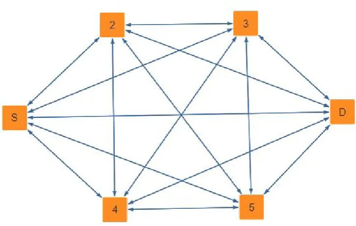
The designed MILP model is tested on several cases in different networks. Starting

with the Complete Unicast Network (a set of 6 Nodes inclusive of a Source node

and a Destination Node with 3 VNFs to be placed among these nodes) as shown in

Figure 1, the following scenarios are tested. The links are shown below:

links = {<1,2>,<1,3>,<1,4>,<1,5>,<1,6>,<1,1>,

<2,1>,<2,3>,<2,4>,<2,5>,<2,6>,<2,2>,

<3,1>,<3,2>,<3,4>,<3,5>,<3,6>,<3,3>,

<4,1>,<4,2>,<4,3>,<4,5>,<4,6>,<4,4>,

<6,1>,<6,2>,<6,3>,<6,4>,<6,5>,<6,6>};

with their respective link costs as:

linkcost = [50,2,1,2,16,0,

50,50,10,3,1,0,

2,50,15,24,50,0,

1,10,15,19,7,0,

2,3,24,19,1,0,

16,1,50,7,1,0];

and the cost of placing the VNF at each Node:

vnfcost = [[3,3,3],

[10,18,10],

[10,10,10],

[18,10,40],

[18,20,10],

[16,25,30]];

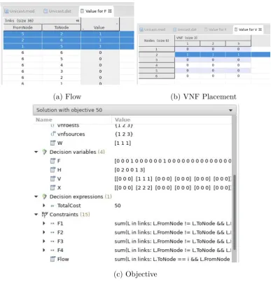
Case 1: No Precedence between VNFs and only VNF 1 and VNF 3 should be placed along the flow from S to D.

In this case, we observed that the Objective is 32, the placement of VNF 1 is

at node 2 and the placement of VNF 3 at node 5. While the path from S to D is

1−>5−>2−>6.

So here, the VNF 3 is placed first and the VNF 1 is placed next. The Figure 2

show the placement, path and the Objective.

Case 2: Precedence between VNFs is chosen as: V N F1−> V N F3−> V N2 Here the Objective is increased to 50, with the same path as the previous case

while the placement of VNFs are changed. Now, we have all the 3 VNFs placed at

Figure 1: Unicast Network

Case 3: This case is with no VNFs, so no Precedence in order to find the cheapest and the best path from S to D.

The resulted objective is very less and is 6 according to the link costs that are

shown above. The path from S to D is 1− > 5− > 6. The VNFs are not placed anywhere which satisfy our condition and the outputs are shown in Figure 4.

As we were able to get the expected outcomes from the Unicast model, we

expanded our interest to Multicast networks and the results from the Multicast

model are shown in the next section.

Multicast Model

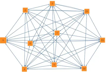
For testing of the Multicast algorithm, we examined a complete 10 Node network

with one Source Node and 3 Destination Nodes along with 3 VNFs as shown in

Figure 5. The links, link costs and vnf costs considered are as below:

links =

{<1,2>,<1,3>,<1,4>,<1,5>,<1,6>,<1,7>,<1,8>,<1,9>,<1,10>,<1,1>,

(a) Flow (b) VNF Placement

(c) Objective

Figure 2: Unicast Results with No Precedence between VNFs

<3,1>,<3,2>,<3,4>,<3,5>,<3,6>,<3,7>,<3,8>,<3,9>,<3,10>,<3,3>,

<4,1>,<4,2>,<4,3>,<4,5>,<4,6>,<4,7>,<4,8>,<4,9>,<4,10>,<4,4>,

<5,1>,<5,2>,<5,3>,<5,4>,<5,6>,<5,7>,<5,8>,<5,9>,<5,10>,<5,5>,

<6,1>,<6,2>,<6,3>,<6,4>,<6,5>,<6,7>,<6,8>,<6,9>,<6,10>,<6,6>,

<7,1>,<7,2>,<7,3>,<7,4>,<7,5>,<7,6>,<7,8>,<7,9>,<7,10>,<7,7>,

<8,1>,<8,2>,<8,3>,<8,4>,<8,5>,<8,6>,<8,7>,<8,9>,<8,10>,<8,8>,

<9,1>,<9,2>,<9,3>,<9,4>,<9,5>,<9,6>,<9,7>,<9,8>,<9,10>,<9,9>,

<10,1>,<10,2>,<10,3>,<10,4>,<10,5>,<10,6>,<10,7>,<10,8>,<10,9>,<10,10>};

(a) Flow (b) VNF Placement

(c) Objective

Figure 3: Unicast Results with VNF Precedence

50,50,10,3,1,7,8,9,10,0,

2,50,5,6,50,7,8,9,10,0,

1,10,5,1,7,7,8,9,10,0,

2,3,6,1,1,7,8,9,10,0,

1,1,50,7,1,7,8,9,10,0,

7,7,7,7,7,7,8,9,10,0,

8,8,8,8,8,8,8,9,10,0,

9,9,9,9,9,9,9,9,10,0,

10,10,10,10,10,10,10,10,10,0];

(a) Flow (b) VNF Placement

(c) Objective

Figure 4: Unicast Results without VNFs

[1,9,7],

[1,8,20],

[3,5,25],

[4,24,4],

[10,10,15],

[8,10,35],

[4,15,19],

[9,90,5],

[16,1,30]];

The similar scenarios that we considered while testing the Unicast model are

implemented here as well.

Figure 5: Multicast Network

a) VNF 1 and VNF 2 for Destination 1 (D1)

b) Only VNF 3 for Destination 2 (D2)

c) VNF 1, VNF 2 and VNF 3 for Destination 3 (D3)

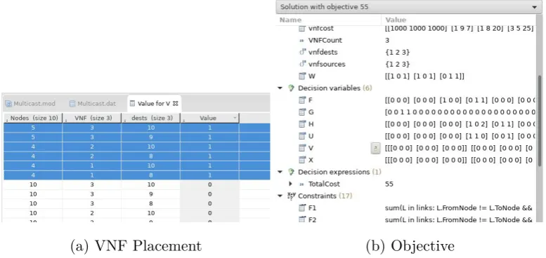
The CPLEX results showed that the placement of VNFs are according to the

requirement with an objective of 55 and the paths for each destination are:

D1: 1−>4−>8 with both VNF 1 and VNF 2 placed at node 4 D2: 1−>4−>9 with VNF 3 placed at node 5

D3: 1−>4−>5−>10 with VNF 1 and VNF 2 placed at node 4 and the VNF 3 placed at node 5

The results for this case from CPLEX are shown in Figure 6.

Case 2: With Precedence between VNFs asV N F3−> V N F1−> V N F2 and the VNF requirement for each destination is same as previous case.

The results are similar. The objective is 55, the VNF placements are same but

(a) VNF Placement (b) Objective

Figure 6: Multicast Results with No Precedence between VNFs

D1: 1−>4−>8 with both VNF 1 and VNF 2 placed at node 4 D2: 1−>4−>9 with VNF 3 placed at node 5

D3: 1−>5−>4−>10 with VNF 1 and VNF 2 placed at node 4 and the VNF 3 placed at node 5

showing that the precedence between VNFs is followed and the CPLEX outputs

are shown in Figure 7.

(a) VNF Placement (b) Objective

Figure 7: Multicast Results with Precedence between VNFs

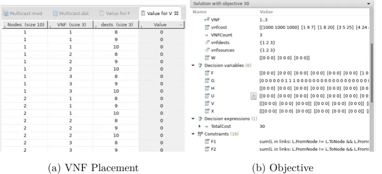
Case 3: In this case, no VNFs and hence no precedence relationship.

The outcome showed the lowest cost for the defined Multicast session with VNFs

are not placed at all as expected. The objective is 30 and the paths are:

D2: 1−>9 D3: 1−>10

The CPLEX results for this case are shown in Figure 8.

(a) VNF Placement (b) Objective

Figure 8: Multicast Results with No VNFs

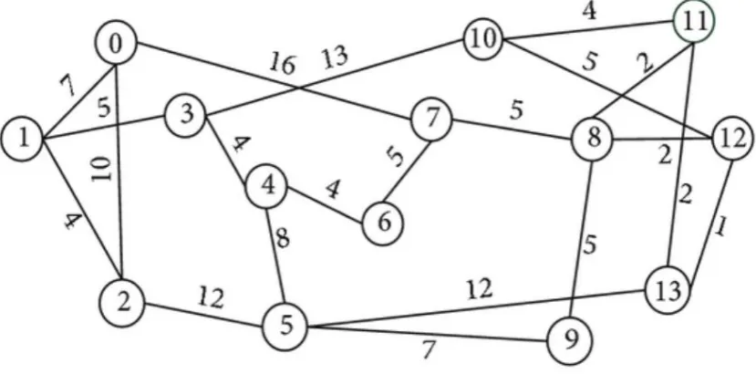
NSF Network Model

In addition to these network topology, we also considered NSF network topology for

our testing purposes. This is a 14 node and 21 bidirectional link model with links

and their costs are shown in Figure 9. This is extracted from reference.

We considered 3 VNFs and 3 destination nodes (11,12 and 13) with the Source

node as 0 while vnf costs at each node are assumed randomly like any other model

and they are shown below:

vnfcost = [[1000,1000,1000],

[1,9,7],

[1,8,20],

[3,5,25],

[4,24,14],

[10,10,15],

[8,10,35],

Figure 9: NSF Network

[5,14,34],

[7,19,17],

[8,16,13],

[4,15,19],

[9,90,5],

[16,1,30]];

We have implemented this model in the similar cases as the previous model and the

different test scenarios are:

Case 1: No Precedence between VNFs and the VNF requirement for each Des-tination are as follows:

a) VNF 1 and VNF 2 for Destination 1 (D1)

b) Only VNF 3 for Destination 2 (D2)

c) VNF 1, VNF 2 and VNF 3 for Destination 3 (D3)

The results are similar and as expected. They are shown in Figure 10.

The output paths are:

D1: 0− >1− >3−> 10− >11 with VNF 1 and VNF 2 placed at nodes 1 and 3 respectively

(a) VNF Placement (b) Objective

Figure 10: NSF Network Model Results with No Precedence between VNfs

D3: 0−>1−>3−>10−>13 with VNF 1 and VNF 3 placed at node 1 and the VNF 2 placed at node 3

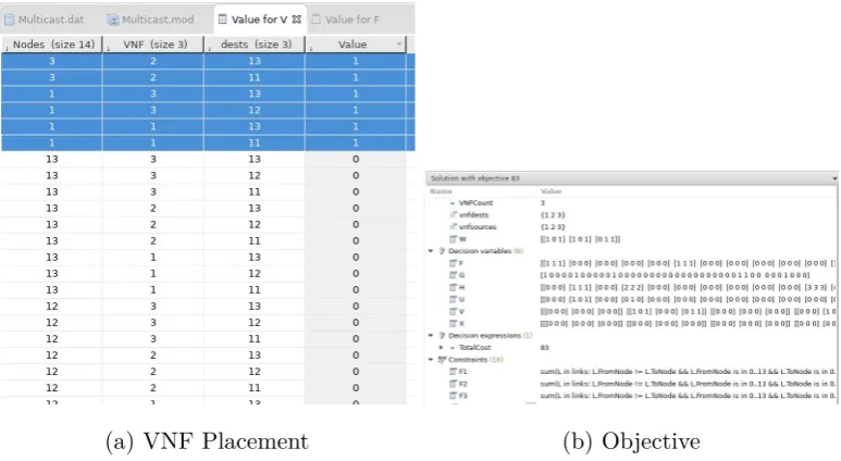
Case 2: With Precedence between VNFs asV N F2−> V N F1−> V N F3 and the VNF requirement for each Destination remains same.

The CPLEX outputs show that the paths are changed and the VNF locations

are also changed with a slight increase in the cost. These are shown in the Figure

11.

(a) VNF Placement (b) Objective

Figure 11: NSF Network Model Results with Precedence between VNfs

D1: 0−>2−>5−>13−>11 with both VNF 1 and VNF 2 placed at node 2 D2: 0−>2−>5−>13−>12 with VNF 3 placed at node 5

D3: 0−>2−>5−>13 with VNF 1 and VNF 2 placed at node 2 and the VNF 3 placed at node 5

Case 3: Here, we consider no VNFs so no precedence also.

As discussed before, this case gives the cheapest path to destinations from Source.

(a) Objective

Figure 12: NSF Network Model Results with No VNFs

The paths from Source to each destination are below:

D1: 0−>7−>8−>11 D2: 0−>7−>8−>12

D3: 0−>7−>8−>12−>13

We can see in every case, the cost of the duplicate links like 0− >7− >8− >

in this case are considered only once. As typically, the path is common from node

6. Conclusion

In this report, we developed an algorithm to place VNFs along the path to the

desti-nations in Multicast Networks. We introduced the allocation of VNFs at nodes with

precedence in the Unicast network. We then advanced our algorithm to Multicast

networks. This algorithm is developed as a MILP model and the optimal solutions

that are obtained for each of the network topology that we considered are shown

in the previous section. The formulation is generalized and ensures an optimal

so-lution also by eliminating the calculation of the duplicate entries for paths or VNF

placements.

Moreover, observing all the cases that we considered for testing with different

network models, we can say that the defined Precedence relationships are followed

between VNFs and these VNFs are placed in the flows to each destinations with the

minimal cost.

With this, we can conclude that the algorithm that we designed for a Multicast

network model is capable of placing VNFs at the Nodes in the Flow by following

the Precedence relationship leading the lowest cost path to destinations.

As a part of our development in this algorithm, we have not included/observed

the performance of VNFs as it is out of the scope of this report. But as a future

improvement to this work, the performance optimization of VNFs can definitely add

Bibliography

[1] ETSI, “NFV: Architectural Framework.” https://www.etsi.org/deliver/

etsi_gs/NFV/001_099/002/01.01.01_60/gs_NFV002v010101p.pdf/.

[2] Wikipedia, “Network Function Virtualization.” https://en.wikipedia.org/

wiki/Network_function_virtualization/.

[3] https://www.electronics-notes.com/articles/

connectivity/nfv-network-functions-virtualisation/

virtualized-network-functions-vnf.php/.

[4] R. Mijumbi, J. Serrat, J. Gorricho, N. Bouten, F. De Turck, and R. Boutaba,

“Network function virtualization: State-of-the-art and research challenges,”

IEEE Communications Surveys Tutorials, vol. 18, pp. 236–262, Firstquarter

2016.

[5] S. Q. Zhang, Q. Zhang, H. Bannazadeh, and A. Leon-Garcia, “Routing

algo-rithms for network function virtualization enabled multicast topology on sdn,”

IEEE Transactions on Network and Service Management, vol. 12, pp. 580–594,

Dec 2015.

[6] T. T. H. Trung V. Phan, Linh H. Ngo and N. H. Thanh, “Optimizing resource

allocation for elastic security vnfs in the sdnfv-enabled cloud computing,” in2017

International Conference on Information Networking (ICOIN), pp. 163–166, Jan

2017.

[7] R. Ul-Mustafa and A. E. Kamal, “Design and provisioning of wdm networks with

multicast traffic grooming,”IEEE Journal on Selected Areas in Communications,

[8] A. M. Hamad and A. E. Kamal, “Optical amplifiers placement in wdm mesh

networks for optical multicasting service support,” J. Opt. Commun. Netw.,

vol. 1, pp. 85–102, Jun 2009.

[9] T. Omar, Z. Abichar, A. E. Kamal, J. M. Chang, and M. A. Alnuem,

“Fault-tolerant small cells locations planning in 4g/5g heterogeneous wireless networks,”