Int. J. Nonlinear Anal. Appl. 11 (2020) No. 1, 7-20 ISSN: 2008-6822 (electronic)
http://dx.doi.org/10.22075/ijnaa.2020.4205
Face Recognition by Cognitive Discriminant Features
Iman Firouzian*, Nematallah Firouzian
Faculty of Computer Engineering and IT, Shahrood University of Technology, Shahrood, Iran; Department of strategic management, Bank Melli Iran, Tehran, Iran;
(Communicated by M. B. Ghaemi)
Abstract
Face recognition is still an active pattern analysis topic. Faces have already been treated as objects or textures, but human face recognition system takes a different approach in face recognition. People refer to faces by their most discriminant features. People usually describe faces in sentences like “She’s snub-nosed” or “he’s got long nose” or “he’s got round eyes” and so like. These most discriminant features have been extracted by comparing a face with average face formed in one’s mind. We have mathematically formulated the approach and placed importance upon the most discriminant features. We have explained feature processing and classification parts in details. We also explained the train and test phases of the proposed algorithm. We have compared the proposed classification part with 1-NN classifier to show the strength of the algorithm and reported the results. We have also compared the whole proposed algorithm with a well-known face recognition method, Eigenfaces and achieved promising results in different cases.
Keywords: Face recognition, Most discriminant features, average face, Cognitive Pattern Recognition.
2010 MSC: 68T45
1. Introduction
Face recognition has absorbed lots of attention and energy from researchers for over 30 years. Since almost no algorithm or combined algorithms is accepted as a general face recognition method with desired time complexity and accuracy in two dimensional still images and videos, the subject is still an ongoing research field in laboratories and research centers. Face recognition methods for still images can be categorized into four main groups such as holistic approaches, feature-based approaches,
∗Iman Firouzian
Email address: [email protected], [email protected] (Iman Firouzian*, Nematallah Firouzian)
8 Iman Firouzian, NematAllah Firouzian
model-based approaches and hybrid approaches. Most of the methods in the face recognition domain have treated faces just as objects or textures such as Eigenfaces[3], Fisherfaces [4], and Laplacianfaces [5], LBP [7], Gabor [6] and wavelet [8]. Faces may have lots of deformations. We are to change the perspective of face recognition methods. We believe a face recognition system must involve human-like descriptions with nominal features. In order to design a system capable of accurately recognizing faces, the system should simulate the way humans recognize faces. Elaborating all aspects of human face recognition mechanism is a hot subject in cognitive psychology and has not been realized completely. We have noticed that people refer to faces by their most discriminant features; human face recognition mechanism extracts some nominal features from faces that can be described. In order to understand this perfectly, ask a person to describe a specific face. People usually describe faces in sentences like “She’s snub-nosed” or “he’s got long nose” or “he’s got round eyes” and so like. What we actually found out is that the descriptions are based on what we consider as a discriminant feature with respect to the average face in a certain geographical region. More specifically, people living in a certain geographical region have created an average face in their minds from the people in that area and whenever they want to describe a face, they refer to most discriminant features with respect to the average face. If the people in that region all have round eyes and so the person in question, it won’t be an appropriate face feature to specify the person but If the people in that region all have long nose while the person in question have broad nose, it can be a discriminant feature to specify the person by. Therefore, the most discriminant face descriptors with respect to regional face average are used to describe and specify a specific person. Extracted face features, regional face average, the deviations of average face and other issues are all fully explained in the section 3. The rest of the paper is organized as follows. Section two presents related works in the face recognition domain. Section three presents the proposed algorithm and the main contribution of the paper. Section four introduces CBF dataset and later on considered assumptions on the database will be explained. In section five, experimental results of the proposed algorithm will be discussed. In section six, conclusion will be discussed.
2. Related Works
Face recognition has always been a challenging and active area of pattern recognition and com-puter vision fields. Face recognition methods for still images can be categorized into four main groups such as holistic approaches, feature-based approaches, model-based approaches and hybrid approaches.
In holistic approaches, the whole face region-of-interest patch is taken as an input to face recog-nition technique. Holistic face approaches utilize global information from faces to perform face recognition. The global information from faces is fundamentally represented by a small number of features which are directly derived from the pixel information of face images. These few features distinctly capture the variance among different individual faces and can be used to uniquely iden-tify individuals. Some examples of this category of methods are Eigenfaces[3], Fisherfaces [4], and Laplacianfaces [5] and Independent Component Analysis (ICA) [9].
The holistic approach has advantages of distinctly capturing the most prominent features within face images used, to uniquely identify individuals amongst a gallery set, as well as, automatically finding features. However, disadvantages of holistic approaches are that recognition performance could be significantly affected by: a probe set deviating from the average face of a gallery set because of lighting, orientation and scale; or, features found from faces may not form part of the face but some other feature captured. For example, capturing features from the background of a face.
Face Recognition by Cognitive Discriminant Features 11 (2020) No. 1, 7-20 9
eyes or nose) [10], [11]. Feature-based face recognition uses a priori information or local features of faces to select a number of features to uniquely identify individuals. Local features include the eyes, nose, mouth, chin and head outline, which are selected from face images.
The advantages for feature-based approaches include the accurate selection of facial features to uniquely identify individuals and its robustness in recognition performance despite variations in face expression, faces being occluded by another object, orientation or lighting. On the other hand, the disadvantages of this approach were that if features were selected manually then this could contain inaccurate location of features by the human user, or, if features were automatically selected then this would be reliant on the accuracy of the feature-based approach, hence leading to inaccurate location of face features.
Model-based approaches try to model a human face. The new sample is ?tted to the model, and the parameters of the ?tted model used to recognize the image. Model-based approaches can be 2-Dimensional or 3-Dimensional. These algorithms try to build a model of a human face. These models are often morphable. A morphable model allows to classify faces even when pose changes are present. 3D models are more complicate, as they try to capture the three dimensional nature of human faces. Examples of this approach are Elastic Bunch Graph Matching or 3D Morphable Models [12, 13, 14, 15, 16].
Cootes et al. [17][18] developed a 2D morphable face model, through which the face variations are learned. A more advanced 3D morphable face model is explored to capture the true 3D structure of human face surface. Both morphable model methods come under the framework of ‘interpretation through synthesis’. The model-based scheme usually contains three steps: 1) Constructing the model; 2)Fitting the model to the given face image; 3) Using the parameters of the fitted model as the feature vector to calculate the similarity between the query face and prototype faces in the database to perform the recognition.
In hybrid approaches, both local features and holistic approaches are together used to better classify and identify faces. Examples of hybrid approaches are modular Eigenfaces, hybrid local feature, shape normalized and component-based methods.
3. Proposed method
3.1. Train phase
10 Iman Firouzian, NematAllah Firouzian International Journal of xxxxxx
Vol. x, No. x, xxxxx, 20xx
4
Figure 1: Sample annotated subject from IMM database.
Figure 2: The mouth with straight lines delineate the mouth of IMM database subject (drawn in Fig. 1). The mouth with dashed lines delineate the average mouth of all subjects in the database. It is obtained by taking the average of the coordinates of
corresponding points of all subjects in the database.
After calculating average facial features, we define a measure of deviation for each subject’s facial feature (e.g. eye) with respect to the corresponding average facial feature (e.g. average eye of the database). This measure of deviation can be defined in different ways; the one that we used here, calculates the difference between Euclidean distances of corresponding points from center; what we mean by center is the average point of all the points of the respective average facial feature (Fig. 3). The deviation can be defined in other ways rather than this way but it should be noted that this deviation should handle stretchiness, roundness, special form of each facial features. The deviation calculation mechanism is defined for every other facial feature such as right eye, left eye, nose and jaw.
Figure 3: Each subject of the database is described by the deviation of its features from the respective average facial feature. In the figure, you can see the points delineating the mouth of subject 1 (Fig. 1) by unfilled circles and average mouth of the database by filled circles. We have specified a center point by taking the average of all filled points and labelled it “center”. The
difference between Euclidean distances of corresponding points from center is defined as deviation.
We compute the deviation of every facial feature (eyes, nose, mouth, jaw) of each subject from the respective average facial feature based on a certain defined measure. Our defined measure outputs a real number. We have calculated the deviation of the nose of each subject from the database average nose and drawn the results in Fig. 4.
Figure 1: Sample annotated subject from IMM database. International Journal of xxxxxx
Vol. x, No. x, xxxxx, 20xx
4
Figure 1: Sample annotated subject from IMM database.
Figure 2: The mouth with straight lines delineate the mouth of IMM database subject (drawn in Fig. 1). The mouth with dashed lines delineate the average mouth of all subjects in the database. It is obtained by taking the average of the coordinates of
corresponding points of all subjects in the database.
After calculating average facial features, we define a measure of deviation for each subject’s facial feature (e.g. eye) with respect to the corresponding average facial feature (e.g. average eye of the database). This measure of deviation can be defined in different ways; the one that we used here, calculates the difference between Euclidean distances of corresponding points from center; what we mean by center is the average point of all the points of the respective average facial feature (Fig. 3). The deviation can be defined in other ways rather than this way but it should be noted that this deviation should handle stretchiness, roundness, special form of each facial features. The deviation calculation mechanism is defined for every other facial feature such as right eye, left eye, nose and jaw.
Figure 3: Each subject of the database is described by the deviation of its features from the respective average facial feature. In the figure, you can see the points delineating the mouth of subject 1 (Fig. 1) by unfilled circles and average mouth of the database by filled circles. We have specified a center point by taking the average of all filled points and labelled it “center”. The
difference between Euclidean distances of corresponding points from center is defined as deviation.
We compute the deviation of every facial feature (eyes, nose, mouth, jaw) of each subject from the respective average facial feature based on a certain defined measure. Our defined measure outputs a real number. We have calculated the deviation of the nose of each subject from the database average nose and drawn the results in Fig. 4.
Figure 2: The mouth with straight lines delineate the mouth of IMM database subject (drawn in Fig. 1). The mouth with dashed lines delineate the average mouth of all subjects in the database. It is obtained by taking the average of the coordinates of corresponding points of all subjects in the database.
After calculating average facial features, we define a measure of deviation for each subject’s facial feature (e.g. eye) with respect to the corresponding average facial feature (e.g. average eye of the database). This measure of deviation can be defined in different ways; the one that we used here, calculates the difference between Euclidean distances of corresponding points from center; what we mean by center is the average point of all the points of the respective average facial feature (Fig. 3). The deviation can be defined in other ways rather than this way but it should be noted that this deviation should handle stretchiness, roundness, special form of each facial features. The deviation calculation mechanism is defined for every other facial feature such as right eye, left eye, nose and jaw.
We compute the deviation of every facial feature (eyes, nose, mouth, jaw) of each subject from the respective average facial feature based on a certain defined measure. Our defined measure outputs a real number. We have calculated the deviation of the nose of each subject from the database average nose and drawn the results in Fig. 4.
International Journal of xxxxxx Vol. x, No. x, xxxxx, 20xx
4
Figure 1: Sample annotated subject from IMM database.
Figure 2: The mouth with straight lines delineate the mouth of IMM database subject (drawn in Fig. 1). The mouth with dashed lines delineate the average mouth of all subjects in the database. It is obtained by taking the average of the coordinates of
corresponding points of all subjects in the database.
After calculating average facial features, we define a measure of deviation for each subject’s facial feature (e.g. eye) with respect to the corresponding average facial feature (e.g. average eye of the database). This measure of deviation can be defined in different ways; the one that we used here, calculates the difference between Euclidean distances of corresponding points from center; what we mean by center is the average point of all the points of the respective average facial feature (Fig. 3). The deviation can be defined in other ways rather than this way but it should be noted that this deviation should handle stretchiness, roundness, special form of each facial features. The deviation calculation mechanism is defined for every other facial feature such as right eye, left eye, nose and jaw.
Figure 3: Each subject of the database is described by the deviation of its features from the respective average facial feature. In the figure, you can see the points delineating the mouth of subject 1 (Fig. 1) by unfilled circles and average mouth of the database by filled circles. We have specified a center point by taking the average of all filled points and labelled it “center”. The
difference between Euclidean distances of corresponding points from center is defined as deviation.
We compute the deviation of every facial feature (eyes, nose, mouth, jaw) of each subject from the respective average facial feature based on a certain defined measure. Our defined measure outputs a real number. We have calculated the deviation of the nose of each subject from the database average nose and drawn the results in Fig. 4.
Face Recognition by Cognitive Discriminant Features 11 (2020) No. 1, 7-20 11 International Journal of xxxxxx
Vol. x, No. x, xxxxx, 20xx
5
Figure 4: the deviations of all subjects’ mouths from average mouth of the database.
Each star in the figure shows a distinct subject. Note that sum of all deviations would not necessarily equal to zero because of the definition of average facial feature. In this paper, we care about the value which deviates more than others from the average. If the difference of one subject’s nose from the average nose was considerably high, then the nose can be an appropriate feature to specify the subject by. As you remember, we tried to simulate a system in which we were looking for some features in subjects that are most discriminant. Suppose a person whose eyes, eyebrows, nose are close to the average respective facial feature but his/her mouth feature is considerably deviated with respect to the deviations of other subject’s mouths; In this case, the mouth feature will be an appropriate discriminating feature for this subject.
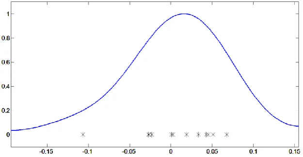
After calculating all the deviations from the average, we tried to estimate the density function of the deviation values in a non-parametric way. Kernel density estimates are closely related to histograms, but can be endowed with properties such as smoothness or continuity by using a suitable kernel. Here, we chose Gaussian kernel to estimate the density function. One of the smoothing parameters of kernel is bandwidth parameter. Bandwidth parameter is a smoothing parameter for the density estimation function; here, bandwidth parameter is set automatically. As you can see in Fig 5, the function is estimated by the deviations of all subjects. The estimation helps up visualize how populated subjects would look like in higher number. the vertical axis can also represent the importance level for the deviation from the average. Since the proposed method states that more deviated subjects are worth more than less deviated subjects in that specific feature, this figure can somehow represent the fact.
Figure 5: estimated density estimation for mouth deviations of all subjects from average mouth of the database.
The importance level can be represented by reversing the estimated density function. As you can see in Fig. 6, if a subject’s deviation from respective average mouth of the database increases, its importance level will rise up accordingly.
Figure 4: The deviations of all subjects’ mouths from average mouth of the database. International Journal of xxxxxx
Vol. x, No. x, xxxxx, 20xx
5
Figure 4: the deviations of all subjects’ mouths from average mouth of the database.
Each star in the figure shows a distinct subject. Note that sum of all deviations would not necessarily equal to zero because of the definition of average facial feature. In this paper, we care about the value which deviates more than others from the average. If the difference of one subject’s nose from the average nose was considerably high, then the nose can be an appropriate feature to specify the subject by. As you remember, we tried to simulate a system in which we were looking for some features in subjects that are most discriminant. Suppose a person whose eyes, eyebrows, nose are close to the average respective facial feature but his/her mouth feature is considerably deviated with respect to the deviations of other subject’s mouths; In this case, the mouth feature will be an appropriate discriminating feature for this subject.
After calculating all the deviations from the average, we tried to estimate the density function of the deviation values in a non-parametric way. Kernel density estimates are closely related to histograms, but can be endowed with properties such as smoothness or continuity by using a suitable kernel. Here, we chose Gaussian kernel to estimate the density function. One of the smoothing parameters of kernel is bandwidth parameter. Bandwidth parameter is a smoothing parameter for the density estimation function; here, bandwidth parameter is set automatically. As you can see in Fig 5, the function is estimated by the deviations of all subjects. The estimation helps up visualize how populated subjects would look like in higher number. the vertical axis can also represent the importance level for the deviation from the average. Since the proposed method states that more deviated subjects are worth more than less deviated subjects in that specific feature, this figure can somehow represent the fact.
Figure 5: estimated density estimation for mouth deviations of all subjects from average mouth of the database.
The importance level can be represented by reversing the estimated density function. As you can see in Fig. 6, if a subject’s deviation from respective average mouth of the database increases, its importance level will rise up accordingly.
Figure 5: Estimated density estimation for mouth deviations of all subjects from average mouth of the database.
Each star in the figure shows a distinct subject. Note that sum of all deviations would not necessarily equal to zero because of the definition of average facial feature. In this paper, we care about the value which deviates more than others from the average. If the difference of one subject’s nose from the average nose was considerably high, then the nose can be an appropriate feature to specify the subject by. As you remember, we tried to simulate a system in which we were looking for some features in subjects that are most discriminant. Suppose a person whose eyes, eyebrows, nose are close to the average respective facial feature but his/her mouth feature is considerably deviated with respect to the deviations of other subject’s mouths; In this case, the mouth feature will be an appropriate discriminating feature for this subject.
After calculating all the deviations from the average, we tried to estimate the density function of the deviation values in a non-parametric way. Kernel density estimates are closely related to histograms, but can be endowed with properties such as smoothness or continuity by using a suitable kernel. Here, we chose Gaussian kernel to estimate the density function. One of the smoothing parameters of kernel is bandwidth parameter. Bandwidth parameter is a smoothing parameter for the density estimation function; here, bandwidth parameter is set automatically. As you can see in Fig 5, the function is estimated by the deviations of all subjects. The estimation helps up visualize how populated subjects would look like in higher number. the vertical axis can also represent the importance level for the deviation from the average. Since the proposed method states that more deviated subjects are worth more than less deviated subjects in that specific feature, this figure can somehow represent the fact.
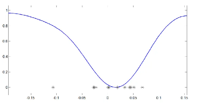
The importance level can be represented by reversing the estimated density function. As you can see in Fig. 6, if a subject’s deviation from respective average mouth of the database increases, its importance level will rise up accordingly.
12 Iman Firouzian, NematAllah Firouzian International Journal of xxxxxx
Vol. x, No. x, xxxxx, 20xx
6
Figure 6: reversed estimated density estimation represents the estimated importance level for different values of deviations.
So far, we’ve constructed an estimated density function for every facial feature (right eye, left eye, right eyebrow, left eyebrow, nose, mouth, jaw). Note that estimated density functions of facial features can be even multimodal and this multimodality property would not cause any problem in the process of method.
3.2. Test phase
Our classifier mechanism is the main contribution of the article and elaborates how a test image will be compared against the database face images. In this section, we also solve the recognition problem with two other classifiers including 1-NN and modified 1-NN in order to show the strength and the power of our proposed method. We express the advantages and disadvantages of the three and elaborate the details by an example. The comparison of our classifier with simple 1-NN and a modified version of 1-NN would help us realizing the mechanism in a step by step process.
At first, we build a table like table 1 which contains all subjects with zero scores. The score of a subject can only increase/decrease according to the likeliness of test image and the subject in each facial feature. In all the next three methods, table 1 is needed in order to accumulate all subjects’ scores.
Table 1: Scores of all subjects are initialized with zero.
Subjects S1 S2 S3 … Sn-1 Sn
Total Scores
0 0 0 … 0 0
Before starting statistical analysis on test image, facial features of the test image must be extracted. After obtaining the contours or points delineating facial features, we calculate the deviation of each facial feature from the respective average facial feature obtained in the training phase.
Consider a classification system with 3 features (Fig. 7 and Fig. 8 and Fig. 9); only two train subjects are considered for simplifying following calculations.
Figure 6: Reversed estimated density estimation represents the estimated importance level for different values of deviations.
Table 1: Scores of all subjects are initialized with zero.
Subjects S1 S2 S3 . . . Sn−1 Sn
Total Scores
0 0 0 . . . 0 0
3.2. Test phase
Our classifier mechanism is the main contribution of the article and elaborates how a test image will be compared against the database face images. In this section, we also solve the recognition problem with two other classifiers including 1-NN and modified 1-NN in order to show the strength and the power of our proposed method. We express the advantages and disadvantages of the three and elaborate the details by an example. The comparison of our classifier with simple 1-NN and a modified version of 1-NN would help us realizing the mechanism in a step by step process.
At first, we build a table like table 1 which contains all subjects with zero scores. The score of a subject can only increase/decrease according to the likeliness of test image and the subject in each facial feature. In all the next three methods, table 1 is needed in order to accumulate all subjects’ scores.
Before starting statistical analysis on test image, facial features of the test image must be ex-tracted. After obtaining the contours or points delineating facial features, we calculate the deviation of each facial feature from the respective average facial feature obtained in the training phase. Consider a classification system with 3 features (Fig. 7 and Fig. 8 and Fig. 9); only two train subjects are considered for simplifying following calculations.
1. Simple 1-NN classifier
In the case which the main classifier is a simple 1-NN, when a test subject comes in, the features of test subject are extracted and should be compared with each of train subjects. In the simple 1-NN classifier, the test subject is labeled as the name of the nearest train subject with the most frequency. In order to classify the test subject, comparison of test subject and train subjects should be done feature by feature.
Face Recognition by Cognitive Discriminant Features 11 (2020) No. 1, 7-20International Journal of xxxxxx 13 Vol. x, No. x, xxxxx, 20xx
7
Figure 7: Right eye feature deviations with estimated density function
Figure 8: Nose feature deviations with estimated density function
Figure 9: Mouth feature deviations with estimated density function
Simple 1-NN classifier
In the case which the main classifier is a simple 1-NN, when a test subject comes in, the features of test subject are extracted and should be compared with each of train subjects. In the simple 1-NN classifier, the test subject is labeled as the name of the nearest train subject with the most frequency. In order to classify the test subject, comparison of test subject and train subjects should be done feature by feature.
In the simple 1-NN classifier algorithm, the nearest train subject with the most frequency to test subject in each feature is desired and should be obtained. The nearest subject to test
Figure 7: Right eye feature deviations with estimated density function
International Journal of xxxxxx Vol. x, No. x, xxxxx, 20xx
7
Figure 7: Right eye feature deviations with estimated density function
Figure 8: Nose feature deviations with estimated density function
Figure 9: Mouth feature deviations with estimated density function
Simple 1-NN classifier
In the case which the main classifier is a simple 1-NN, when a test subject comes in, the features of test subject are extracted and should be compared with each of train subjects. In the simple 1-NN classifier, the test subject is labeled as the name of the nearest train subject with the most frequency. In order to classify the test subject, comparison of test subject and train subjects should be done feature by feature.
In the simple 1-NN classifier algorithm, the nearest train subject with the most frequency to test subject in each feature is desired and should be obtained. The nearest subject to test
Figure 8: Nose feature deviations with estimated density function
International Journal of xxxxxx Vol. x, No. x, xxxxx, 20xx
7
Figure 7: Right eye feature deviations with estimated density function
Figure 8: Nose feature deviations with estimated density function
Figure 9: Mouth feature deviations with estimated density function
Simple 1-NN classifier
In the case which the main classifier is a simple 1-NN, when a test subject comes in, the features of test subject are extracted and should be compared with each of train subjects. In the simple 1-NN classifier, the test subject is labeled as the name of the nearest train subject with the most frequency. In order to classify the test subject, comparison of test subject and train subjects should be done feature by feature.
In the simple 1-NN classifier algorithm, the nearest train subject with the most frequency to test subject in each feature is desired and should be obtained. The nearest subject to test
14 Iman Firouzian, NematAllah Firouzian
Table 2: 1-NN classifier for features extracted out of face
Feature Number Nearest train subject
name
Feature 1 B
Feature 2 A
Feature 3 A
Table 3: Modified 1-NN classifier for features extracted out of face Feature Number Negative form of distances
between test subject and train subjects
Accumulative negative form of distances between test subject and train subjects
Feature 1 A = -0.05, B = -0.01 A = -0.05, B = -0.01
Feature 2 A= -0.02, B = -0.085 A= -0.07, B = -0.095
Feature 3 A= -0.16, B = -0.76 A= -0.28, B = -0.865
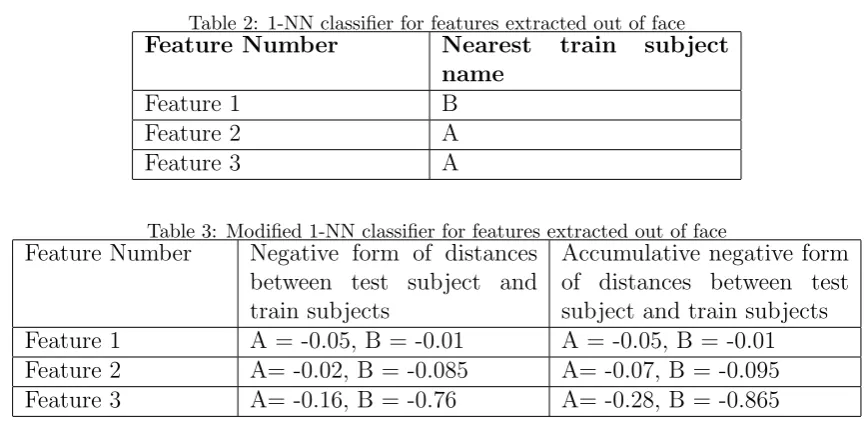
to test subject in Fig 9. is subject A. Since the test subject is labeled as the name of the nearest train subject with the most frequency, it is concluded that test subject is subject A.
1. Modified 1-NN classifier
Since in a simple 1-NN classifier, the number of labels is just important and some data will remain useless, the necessity of using another classifier became clear.
A little more advanced type of 1-NN algorithm also involves the distance between features of test subject and each train subjects. We use negative score here; distances carry negative sign because the less the distance, the less negative value should be assigned to the related train subject feature. We add the negative form of distance to total scores of train subject.
When a test subject comes in, the distance of test subject with each train subject in every feature is calculated. Test subject is labeled as the train subject with the least accumulative negative scores. As you can see in the table below, in the second column negative form of distances between test subject and each of the train subjects (in this case 2 train subjects) are given; In the third column the accumulative result of column 2 is given. At the last row of third column, A has scored more points than B, so the test subject is labeled as A.
1. Our proposed classifier
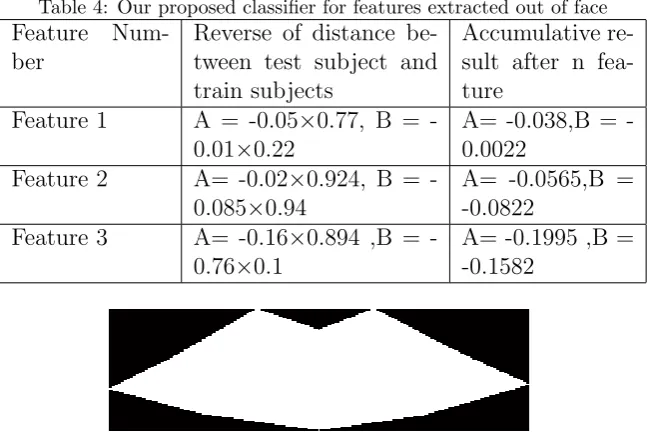
The modified 1-NN has an advantage over simple 1-NN by involving distances between test subject and train subjects but still has a problem of not involving other existing data. Our proposed method not only involves the distance between test subject and each train subject, but also involves the estimated density function. Our proposed method supports the idea that if a feature of a train subject is more deviated than others, it should be considered as an important discriminant feature. This importance level is defined by the reversed estimated density function. The reversed estimated density function expresses the fact that features in low density range are more important than features in high density range because of the most discriminancy factor explained earlier.
Face Recognition by Cognitive Discriminant Features 11 (2020) No. 1, 7-20 15
Table 4: Our proposed classifier for features extracted out of face Feature
Num-ber
Reverse of distance be-tween test subject and train subjects
Accumulative re-sult after n fea-ture
Feature 1 A = -0.05×0.77, B = -0.01×0.22
A= 0.038,B = -0.0022
Feature 2 A= -0.02×0.924, B = -0.085×0.94
A= -0.0565,B = -0.0822
Feature 3 A= -0.16×0.894 ,B = -0.76×0.1
A= -0.1995 ,B = -0.1582
International Journal of xxxxxx Vol. x, No. x, xxxxx, 20xx
9
low density range are more important than features in high density range because of the most discriminancy factor explained earlier.
Since, we want to make important features to get higher scores and therefore less negative scores, the estimated density function for each feature of all subjects is calculated and is multiplied by the negative form of distances. For example the value of feature 1 (Fig. 7) of subject A in estimated density function is 0.23 and it’s multiplied by the negative distance between the first feature of test subject and the first feature of each train subject. This will be applied to other features as well. At last, test subject is labeled as the label of the train subject with maximum accumulative value. You can see in the table below that B is has less negative score than A and consequently the test subject is labeled as B.
Table 4:Our proposed classifier for features extracted out of face
Feature Number Reverse of distance between test
subject and train subjects
Accumulative result after n feature
Feature 1 A = -0.050.77, B = -0.010.22 A= -0.038,B = -0.0022
Feature 2 A= -0.020.924, B = -0.0850.94 A= -0.0565,B = -0.0822
Feature 3 A= -0.160.894 ,B = -0.760.1 A= -0.1995 ,B = -0.1582
3.3. Auxiliary geometric features
So far, we’ve used the coordinates of the points surrounding facial features as features (like in Fig.1). We can further improve our system by using other category of features. Since a contour is specified for each facial feature and this contour makes a specific shape, geometric features can be used to extract some auxiliary features to better perform classification and recognition. The shape of a mouth of a subject is drawn below as a sample.
Figure 10: Sample mouth contour has formed a shape; some geometric features are assigned to this shape.
As you can see in the picture above, the shape of mouth has geometrical features. The name of shape features used in this paper are provided below with a short description of each:
1. Area: The actual number of pixels in the region.
2-3.Bounding Box: The smallest rectangle containing the region. This features outputs two numbers to represent the rectangle and is considered as two features.
4-5.Centroid: Vector that specifies the center of mass of the region. This centroid feature includes x and y coordinates and therefore is considered as two features.
6. Eccentricity: The eccentricity is the ratio of the distance between the foci of the ellipse and its major axis length. The value is between 0 and 1. 0 and 1 are degenerate cases; an ellipse whose eccentricity is 0 is actually a circle, while an ellipse whose eccentricity is 1 is a line segment.
Figure 10: Sample mouth contour has formed a shape; some geometric features are assigned to this shape.
subject and the first feature of each train subject. This will be applied to other features as well. At last, test subject is labeled as the label of the train subject with maximum accumulative value. You can see in the table below that B is has less negative score than A and consequently the test subject is labeled as B.
3.3. Auxiliary geometric features
So far, we’ve used the coordinates of the points surrounding facial features as features (like in Fig.1). We can further improve our system by using other category of features. Since a contour is specified for each facial feature and this contour makes a specific shape, geometric features can be used to extract some auxiliary features to better perform classification and recognition. The shape of a mouth of a subject is drawn below as a sample.
As you can see in the picture above, the shape of mouth has geometrical features. The name of shape features used in this paper are provided below with a short description of each:
1. Area: The actual number of pixels in the region.
(a) Bounding Box: The smallest rectangle containing the region. This features outputs two numbers to represent the rectangle and is considered as two features.
(b) Centroid: Vector that specifies the center of mass of the region. This centroid feature includes x and y coordinates and therefore is considered as two features.
2. Eccentricity: The eccentricity is the ratio of the distance between the foci of the ellipse and its major axis length. The value is between 0 and 1. 0 and 1 are degenerate cases; an ellipse whose eccentricity is 0 is actually a circle, while an ellipse whose eccentricity is 1 is a line segment. 3. Extent: The ratio of pixels in the region to pixels in the total bounding box and is computed
as the Area divided by the area of the bounding box.
4. Equivalent Diameter: This parameter specifies the diameter of a circle with the same area as the region which is computed by sqrt(4*Area/pi).
16 Iman Firouzian, NematAllah Firouzian International Journal of xxxxxx
Vol. x, No. x, xxxxx, 20xx
10
7. Extent: The ratio of pixels in the region to pixels in the total bounding box and is computed as the Area divided by the area of the bounding box.
8. Equivalent Diameter: This parameter specifies the diameter of a circle with the same area as the region which is computed by sqrt(4*Area/pi).
9. Major axis length: The length (in pixels) of the major axis of the ellipse that has the same normalized second central moments as the region.
10. Orientation: The angle (in degrees ranging from -90 to 90 degrees) between the x-axis and the major x-axis of the ellipse that has the same second-moments as the region.
We make a vector of 10 shape features for each of the 7 facial features (right eye, left eye, right eyebrow, left eyebrow, nose, mouth, jaw); therefore, each subject has a total of 70 geometric features which are used as auxiliary features to better classify and recognize. These features along with other features explained earlier would be an input to the classifier.
To better understand the usage of geometrical features, we draw the estimated density function for eccentricity feature of right eyebrows of all subjects in the database; Eccentricity features of right eyebrows is just a sample and other 69 geometric features could have been chosen, too. There exist 70 estimated density functions for all 70 geometric features. Note that we have five samples for each of twelve distinct subjects.
Figure 11: Estimated density function for eccentricity feature of right eyebrows of all subjects.
When a test subject comes in, first, facial features must be extracted. Then, geometric features of facial features must be calculated. Each geometric feature of the test subject is compared against features of other subjects. Distances between test subject and train subjects should be calculated. Distances should be signed negative and then multiplied by estimated density values of train subjects. Test subject is labeled as the label of a train subject with the least negative value (most scored).
3.4. Other possible features
We have designed our proposed method so flexible that almost any feature would be acceptable. As an example, even facial moles can be used as a feature; as explained earlier, the features of facial moles of all subjects should be averaged. This averaging operation can
Figure 11: Estimated density function for eccentricity feature of right eyebrows of all subjects.
6. Orientation: The angle (in degrees ranging from -90 to 90 degrees) between the x-axis and the major axis of the ellipse that has the same second-moments as the region.
We make a vector of 10 shape features for each of the 7 facial features (right eye, left eye, right eyebrow, left eyebrow, nose, mouth, jaw); therefore, each subject has a total of 70 geometric features which are used as auxiliary features to better classify and recognize. These features along with other features explained earlier would be an input to the classifier.
To better understand the usage of geometrical features, we draw the estimated density function for eccentricity feature of right eyebrows of all subjects in the database; Eccentricity features of right eyebrows is just a sample and other 69 geometric features could have been chosen, too. There exist 70 estimated density functions for all 70 geometric features. Note that we have five samples for each of twelve distinct subjects.
When a test subject comes in, first, facial features must be extracted. Then, geometric features of facial features must be calculated. Each geometric feature of the test subject is compared against features of other subjects. Distances between test subject and train subjects should be calculated. Distances should be signed negative and then multiplied by estimated density values of train subjects. Test subject is labeled as the label of a train subject with the least negative value (most scored).
3.4. Other possible features
We have designed our proposed method so flexible that almost any feature would be acceptable. As an example, even facial moles can be used as a feature; as explained earlier, the features of facial moles of all subjects should be averaged. This averaging operation can be defined in various ways. We can define the averaging operation by taking the average of locations and sizes of the moles. Suppose only four subjects out of thirty subjects have moles on their face and others do not; As you know, the proposed method highly focuses on discriminancy factor and this mole feature would be an appropriate discriminant feature for the three subjects who have the mole.
Face Recognition by Cognitive Discriminant Features 11 (2020) No. 1, 7-20 17 International Journal of xxxxxx
Vol. x, No. x, xxxxx, 20xx
11
be defined in various ways. We can define the averaging operation by taking the average of locations and sizes of the moles. Suppose only four subjects out of thirty subjects have moles on their face and others do not; As you know, the proposed method highly focuses on discriminancy factor and this mole feature would be an appropriate discriminant feature for the three subjects who have the mole.
Moles are just one sample feature of the possible features. There can be defined lots of features like nasal root wrinkles, forehead wrinkles and freckles and any other feature applicable and has the potential of discriminancy.
4. Results
In this section, we first describe IMM frontal face database and then explain and discuss the obtained results of the proposed algorithm on the database.
4.1. IMM Frontal Face Database
This database consists of 12 people (all male). A total of 10 frontal face photos has been recorded of each person. The dataset is containing different facial poses captured over a short period of time, with a minimum of variance in lighting, camera position, etc. All photos are annotated with landmarks defining the eyebrows, eyes, nose, mouth and jaw, see Fig. 11.
Figure 12: Sample IMM face database image with 73 landmarks annotation defining facial features; eyebrows, eyes, nose, mouth and jaw.
Each subject has 10 photos; 6 of which expresses subject in neutral facial expression, 2 of which expresses subject in relaxed happy facial expression, 2 of which expresses subject in relaxed thinking facial expression. Since facial expression is not the main issue of the paper, we just use the six photos of neutral facial expression of each subject.
4.2. Results and discussion
We have set 5 photos of each of 12 subjects as training set and 1 photo of each as test set. In total, there are 70 photos in the training set and 12 photos in the test set.
When the proposed algorithm (extracted geometric features + proposed classifier) is applied to the database, the accuracy reaches 100%, while the accuracy of 1-NN classifier with the same geometric
Figure 12: Sample IMM face database image with 73 landmarks annotation defining facial features; eyebrows, eyes, nose, mouth and jaw.
4. 4. Results
In this section, we first describe IMM frontal face database and then explain and discuss the obtained results of the proposed algorithm on the database.
4.1. IMM Frontal Face Database
This database consists of 12 people (all male). A total of 10 frontal face photos has been recorded of each person. The dataset is containing different facial poses captured over a short period of time, with a minimum of variance in lighting, camera position, etc. All photos are annotated with landmarks defining the eyebrows, eyes, nose, mouth and jaw, see Fig. 11.
Each subject has 10 photos; 6 of which expresses subject in neutral facial expression, 2 of which expresses subject in relaxed happy facial expression, 2 of which expresses subject in relaxed thinking facial expression. Since facial expression is not the main issue of the paper, we just use the six photos of neutral facial expression of each subject.
4.2. Results and discussion
We have set 5 photos of each of 12 subjects as training set and 1 photo of each as test set. In total, there are 70 photos in the training set and 12 photos in the test set.
When the proposed algorithm (extracted geometric features + proposed classifier) is applied to the database, the accuracy reaches 100%, while the accuracy of 1-NN classifier with the same geometric features would be 75%. Note that in both experiments, only the geometric features are used. The 25% of difference in accuracy would be the best proof to show the strength of our proposed algorithm.
Note that in both experiments, only the geometric features are used. The 25% of difference in accuracy would be the best proof to show the strength of our proposed algorithm.
18 Iman Firouzian, NematAllah Firouzian
Table 5: Results of methods in leave-one-out cross validation
Method Accuracy
Geometric features + proposed classifier
100%
Geometric features + 1-NN classifier
75%
First category of features without geometric features + proposed classifier
91.66%
First category of fea-tures without geo-metric features + 1-NN classifier
91.66%
Eigenfaces 1st rank = 66.67%
2nd rank = 83.33% 3rd rank = 100%
algorithm never doubted between true answer and wrong answer and chose the wrong answer with certainty.
Since lots of papers has presented different methods in face recognition domain, it is expected that our results will be compared with the results of an acceptable and well-known method in face recognition domain. We’ve implemented Eigenfaces method on IMM database and achieve the results. Eigenfaces method has reached the accuracy of 66.67% in rank-1 and 83.33% in rank-2 and 100% in rank-3 and higher.
We have chosen another division for train set and test set. In this case, 4 photos of each of 12 subjects are used as training set and 2 photo of each is used for test set. In total, there are 48 photos in the training set and 24 photos in the test set. We’ve put all the results into the table below.
5. Conclusion
This paper expressed the fact that human facial recognition system extract features which are most discriminant with respect to the average face formed in one’s mind by taking the average of all of the seen faces in the certain geographical region. This fact has been mathematically formulated by extracting features of all kind from the face (In this paper, first category of features and geometric features of each facial feature), taking the average for each facial feature and calculating deviations of all features from average, calculating the estimated density function for deviations. When a test subject comes in, deviations of features of test subject is calculated and is compared with each train subject. The detailed explanation has been fully discussed in the proposed section.
The contribution of the paper includes two parts: feature processing and classification. To show the strength of classification, we’ve classified extracted features with 1-NN; the results prove the predominance of the proposed classification algorithm part over 1-NN. To show the strength of the whole proposed algorithm, we’ve compared the results with the results of a well-known face recognition method, Eigenfaces. The proposed algorithm is superior to rank-1 and rank-2 eigenfaces method.
Face Recognition by Cognitive Discriminant Features 11 (2020) No. 1, 7-20 19
of applying the proposed algorithm to other well-known databases. It is also notable that more features can be extracted to further improve the recognition system.
6. References
[1] Xu, Weilin, David Evans, and Yanjun Qi. ”Feature squeezing: Detecting adversarial examples in deep neural networks.” arXiv preprint arXiv:1704.01155, 2017.
[2] Learned-Miller, Erik, Gary B. Huang, Aruni RoyChowdhury, Haoxiang Li, and Gang Hua. ”La-beled faces in the wild: A survey.” In Advances in face detection and facial image analysis, pp. 189-248. Springer, Cham, 2016.
[3] M. Turk and A. Pentland, “Eigenfaces for Recognition,” Proc. IEEE Int’l Conf. Computer Vision and Pattern Recognition, 1991.
[4] P. Belhumeur, J. Hespanda, and D. Kriegman, “Eigenfaces versus Fisherfaces: Recognition Using Class Specific Linear Projection,” IEEE Trans. Pattern Analysis and Machine Intelligence, vol. 19, no. 7, pp. 711-720, July 1997.
[5] X. He, S. Yan, Y. Hu, P. Niyogi, and H. Zhang, “Face Recognition Using Laplacianfaces,” IEEE Trans. Pattern Analysis and Machine Intelligence, vol. 27, no. 3, pp. 328-340, Mar. 2005.
[6] LinLin Shen, Li Bai: A review on Gabor wavelets for face recognition. Pattern Anal. Appl. 9(2-3): 273-292 (2006)
[7] Ahonen, T., Hadid, A., and Pietikainen, M. Face Recognition with Local Binary Patterns. Com-puter Vision - ECCV 2004 (2004), 469–481.
[8] christophe Garcia, G. Zikos, George Tziritas: Wavelet packet analysis for face recognition. Image Vision Comput. 18(??): 289-297 (2000)
[9] Hyv¨arinen A, Oja E. Independent component analysis: algorithms and applications. Neural Netw 2000;13:411–30
[10] P. Sinha, B. Balas, Y. Ostrovsky, and R. Russell, “Face Recognition by Humans: Nineteen Results All Computer Vision Researchers Should Know about,” Proc. IEEE, vol. 94, no. 11, pp. 1948-1962, 2006.
[11] M. Savvides, R. Abiantun, J. Heo, S. Park, C. Xie, and B. Vijayakumar, “Partial and Holis-tic Face Recognition on FRGC-II Data Using Support Vector Machine Kernel Correlation Feature Analysis,” Proc. Conf. Computer Vision and Pattern Recognition Workshop (CVPR), 2006.
[12] V. Blanz and T. Vetter. A morphable model for the synthesis of 3d faces. In Proc. of the SIGGRAPH’99, pages 187–194, Los Angeles, USA, August 1999.
[13] V. Blanz and T. Vetter. Face recognition based on ?tting a 3d morphable model. IEEE Trans-actions on Pattern Analysis and Machine Intelligence, 25(??):1063–1074, September 2003.
[14] J. Huang, B. Heisele, and V. Blanz. Component-based face recognition with 3d morphable models. In roc. of the 4th International Conference on Audio- and Video-Based Biometric Person Authentication, AVBPA, pages 27–34, Guildford, UK, June 2003.
[15] J. Lee, B. Moghaddam, H. P?ster, and R. Machiraju. inding optimal views for 3d face shape modeling. In Proc. of the International Conference on Automatic Face and Gesture Recognition, FGR2004, pages 31–36, Seoul, Korea, May 2004.
[16] B. Moghaddam, J. Lee, H. P?ster, and R. Machiraju. Model-based 3d face capture with shape-from-silhouettes. In Proc. of the IEEE International Workshop on Analysis and Modeling of Faces and Gestures, AMFG, pages 20–27, Nice, France, October 2003.
20 Iman Firouzian, NematAllah Firouzian