ISSN: 2008-6822 (electronic)
http://dx.doi.org/10.22075/ijnaa.2017.1538.1402
Multiple solutions of a nonlinear reactive transport
model using least square pseudo-spectral collocation
method
Elyas Shivanian, Saeid Abbasbandy∗
Department of Applied Mathematics, Faculty of Basic Science, Imam Khomeini International University, Qazvin 34149–16818, Iran
(Communicated by M. Eshaghi)
Abstract
The recognition and the calculation of all branches of solutions of the nonlinear boundary value problems is difficult obviously. The complexity of this issue goes back to the being nonlinearity of the problem. Regarding this matter, this paper considers steady state reactive transport model which does not have exact closed–form solution and discovers existence of dual or triple solutions in some cases using a new hybrid method based on pseudo–spectral collocation in the sense of least square method. Furthermore, the method usages Picard iteration and Newton method to treat nonlinear term in order to obtain unique and multiple solutions of the problem, respectively.
Keywords: Pseudo–spectral collocation method, Least square method, Newton iteration method, Picard iteration, Chebyshev–Gauss–Lobatto points.
2010 MSC: Primary 65L10; Secondary 34L05.
1. Preliminaries and problem formulation
Chebyshev polynomials [20] are extremely functional as orthogonal polynomials on the interval
[−1,1]. These polynomials which appear frequently in several fields of mathematics, physics and
engineering have very good properties in the approximation of functions. Spectral collocation meth-ods [10, 23] based on Chebyshev polynomials (also is called pseudo-spectral method) in the context of numerical schemes for differential equations, belong to the family of weighted residual methods
∗Corresponding author
Email addresses: [email protected](Elyas Shivanian),[email protected](Saeid Abbasbandy)
(WRMs), which are traditionally regarded as the foundation of many numerical methods such as finite element, spectral, finite volume, boundary element [14]. Spectral collocation methods have been widely used to solve numerically differential equations by many authors, (see for instance [8, 12, 16, 18]). This method is accomplished successfully by generating approximations for the higher–order derivatives through successive differentiation of the approximate solution.
The least square method is a fundamental notion in the theory of approximation [9]. In general, the study of approximation theory involves two general types of problems. One problem arises when a function is given explicitly, but we wish to find a simpler type of function, such as polynomial, that can be used to determine approximated values of the given function. The other problem in approximation theory is concerned with fitting functions to given data and finding the best function in a certain class to represent the data.
It is common that numerical methods usually converge to only one solution that is exactly meaning of convergence. Once the given nonlinear boundary value problem admits multiple solutions, it is consequential to gain all branches of solutions in engineering and physical sciences [2, 3, 5]. Based on this important matter the present paper is going to present a procedure based on pseudo–spectral in the sense of least square using Picard and Newton iteration method to obtain unique, dual and triple solutions of a kind of generalization of the nonlinear reaction–diffusion model in porous catalysts so called one dimensional steady state reactive transport model in some cases.
The governing boundary value problem of the one dimensional steady state reactive transport model can be written in dimensional variables as
DU00−VU0−r(U) = 0, 0≤x≤L, U0(0) = 0, U(L) = Us, (1.1)
where D is the diffusivity, V is the advective velocity and r(U) denotes reaction process [7, 11,
13, 15, 24]. Now, by introducing nondimensional quantities U(x) = UU(X)
s , x =
X
L and R(U) as
nondimensional reaction term and then substituting these nondimensional quantities into equation (1.1), we get
U00−P U0−R(U) = 0, 0≤x≤1, U0(0) = 0, U(1) = 1, (1.2)
where P = V LD is so–called P´eclet number. Without advective transport, we have P = 0 and in this
case the model has been used to study porous catalyst pellets as the model of diffusion and reaction
[13, 22]. Furthermore, if we consider R(U) as Michaelis–Menten reaction term then the model is
converted to
U00(x)− αU(x)
β+U(x) = 0, 0≤x≤1, (1.3)
with the boundary condition
U0(0) = 0, U(1) = 1, (1.4)
where α, characteristic reaction rate, and β is half saturation concentration. The problem (1.2)
without advective transport (P = 0) and with reaction term R(U) = φ2Un (φ is Thiele modulus)
has been studied by Adomian decomposition method [21] and Homotopy analysis method [1, 2]. Subsequently, S. Abbasbandy and E. Shivanian [4] have considered almost the same problem arising in heat transfer and have successfully obtained the exact analytical solution in the implicit form and
proved the existence of dual solutions on some domain of x.
2. Solution Procedure
By the change of variable
x= 1
we get Uxx = 4uηη, then the problem (1.3)–(1.4) can be written as the differential equation with
boundary conditions on interval [−1,1], i.e.
uηη−
α
4βu=−
1
βuuηη, β 6= 0 (2.1)
uη(−1) = 0, u(1) = 1. (2.2)
So, as x goes from zero to one in the original problem continuously, η goes from −1 to 1 as well in
the above differential equation, continuously. Now, having boundary conditions at interval [−1,1],
we apply pseudo–spectral collocation method to handle the above problem as follows:
2.1. Pseudo–spectral collocation method
The method involves using the Chebyshev–Gauss–Lobatto point to discrete interval [−1,1], namely
ηj = cos
πj N
, j = 0,1,2, . . . , N.
The unknown function u(η) is approximated as a truncated series of Chebyshev polynomials
u(η) = N
X
k=0
˜
ukTk(η),
where Tk(η) is the kth Chebyshev polynomial and ˜uk are the Chebyshev coefficients which are
determined by the formulations
˜
uk = 2
Nc˜k N
X
i=0
1 ˜
ci
u(ηi) cos
πik N
, k = 0,1,2, . . . , N,
where
˜
ck =
2, k = 0,
1, 1≤k ≤N,
2, k =N.
As it is well–known in Chebyshev pseudo–spectral method, first and second derivatives of the function
u(η) at the collocation points are presented as
du
dη(ηj) =
N
X
i=0
Diju(ηj), (2.3)
d2u
dη2(ηj) =
N
X
i=0 D2
iju(ηj). (2.4)
In the above equations D is the Chebyshev differentiation matrix and N + 1 is the number of
collocation points (nodes). The entries of the differentiation matrixD are
Dij =− 1 2
˜
ci ˜
cj
(−1)i+j
sinπ(2jN+i)sinπ(2jN−i)
, i6=j
Dii=− 1 2
ηi
sin2 2πiN, i6= 0, N, D00=−DN N =
2N2+ 1
By employing derivatives formulation (2.3)–(2.4), equations (2.1)–(2.2) are transformed to the fol-lowing expressions
u(η0) = 1, PN
j=0D 2
iju(ηj)− 4αβu(ηi) = −1βu(ηi)
PN
j=0D 2
iju(ηj), i= 1,2, . . . , N −1,
PN
j=0DN ju(ηj) = 0.
(2.5)
Equation (2.5) is actually a system of nonlinear equations with number ofN+ 1 equations andN+ 1
unknown parameters u(η0), u(η1), u(η2), . . . , u(ηN).
2.2. Multiple solutions of the model
The recognizability and the computation of all branches of solutions of nonlinear boundary value problems is a major topic in general. This part is devoted to show that the problem (2.1)–(2.2) and so, the original equations (1.3)–(1.4) admit unique or dual or even more, triple solutions for some values of the characteristic reaction rate, and half saturation concentration.
2.2.1. Unique solution–Picard iteration method
Consider the system (2.5) in the following matrix form
LU(η) =−1
βU
0(η)◦ D02
U(η),
where ”◦” denotes the Hadamard product, U(η) = (u(η0), u(η1), u(η2), . . . , u(ηN)) t and L=
1 0 0 · · · 0 0
D2
10 D211− 4αβ D
2
12 · · · D21(N−1) D 2 1N
D2
20 D221 D222−
α
4β · · · D
2
2(N−1) D 2 2N ..
. ... ... . .. ... ...
D2
(N−1)0 D(2N−1),1 D(2N−1)2 · · · D(2N−1)(N−1)−
α
4β D
2 (N−1)N
DN0 DN1 DN2 · · · DN(N−1) DN N
.
Also,D02
=D2 except that D02
00 =−β and D0 2
0j = 0 for all 1≤j ≤N and
U0(η)j =
1 j = 0,
U(η)j 1≤j ≤N −1.
0 j =N.
Now, we provide a detailed description of the proposed nonlinear iterative method. The solution process known as Picard iterative method is as follows:
step 1. Choose an initial guess, U0(η) to the nonlinear system (2.5). step 2. Linearize the nonlinear system (2.5) in terms of U(η).
step 3. Solve the linear system by appropriate method. The above three steps suggests the following process
Un+1(η) = 1
βL
−1hU0
n(η)◦ D
02
Un(η)
i
2.2.2. Multiple solutions–Newton iteration method
It is worth to mention that it is so difficult generally to solve system of nonlinear equations (2.5) even by Newton’s method [17, 19]. The main difficulty with a such system is that how we can choose initial guess to handle Newton’s method, in other words how many solutions the system of nonlinear equations admit. We think the appropriate way to discover proper initial guess (or initial
guesses) is to solve system analytically for very smallN (by using symbolic softwares’ programs such
as Mathematica or Maple) and then we can guess proper initial guesses and particularly multiplicity of solutions of such system, of course, if they converge to different solutions [6]. For example, let us
take N = 3 in system (2.5), then havingu(η0) = 1 we stand to solve
u(η1)(−3α−8(8u(η1)−4u(η2) +u(η3)−5)) + 8β(8u(η1)−4u(η2) +u(η3)−5) = 0, u(η2)(8(4u(η1)−8u(η2) + 5u(η3)−1)−3α) + 8β(4u(η1)−8u(η2) + 5u(η3)−1) = 0, −8u(η1) + 24u(η2)−19u(η3) + 3 = 0.
If we chooseα = 0.5 andβ =−0.1, then after usingη= 2x−1 in Chebyshev polynomial interpolation,
we get two initial guesses as follow (plotted in Figure 1)
U0(x) = 2x
(2x−2)
0.2056−0.0659
2x− 1
2
+ 0.4772
+ 0.0454,
U0(x) = 2x
(2x−2)
0.0718−0.0006
2x− 1
2
+ 0.1442
+ 0.7115,
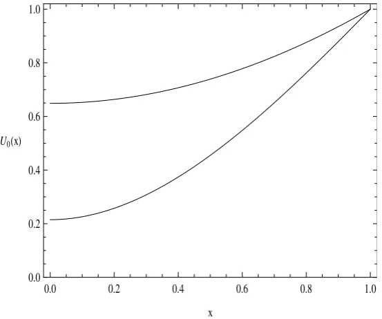
if α= 0.5 and β =−0.2, then we have two other initial guesses (plotted in Figure 2)
U0(x) = 2x
(2x−2)
0.1744−0.0436
2x− 1
2
+ 0.3925
+ 0.2149,
U0(x) = 2x
(2x−2)
0.0865−0.0024
2x− 1
2
+ 0.1755
+ 0.6488,
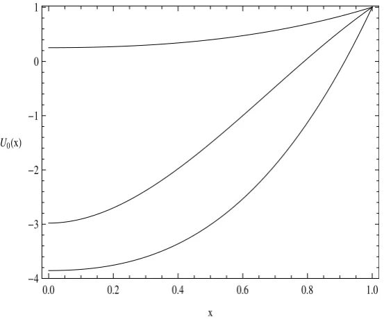
and if we getα= 6 and β = 1, then we are led to three initial guesses as follow (plotted in Figure 3)
U0(x) = 2x
(2x−2)
0.3698
2x− 1
2
+ 1.3986
+ 2.4274
−3.8549,
U0(x) = 2x
(2x−2)
0.7571−0.4758
2x−1
2
+ 1.99
−2.9801,
U0(x) = 2x
(2x−2)
0.0409
2x−1
2
+ 0.2071
+ 0.3733
+ 0.2533.
Now, what it remains is to solve the following linear system iteratively:
JF(Un(η))(Un+1(η)−Un(η)) =−F(Un(η)), (2.7)
where
F(Un(η)) =LU(η) + 1
βU
0
(η)◦ D02U(η)
and JF(Un(η)) is the Jacobian matrix ofF(Un(η)) which is in factJF(Un(η)) =L+ 1βN(η) with
N(η) =
0 0 · · · 0 0
u(η1)D2
10 u(η1)D211+ PN
j=0D12ju(ηj) · · · u(η1)D1(2N−1) u(η1)D21N
u(η2)D2
20 u(η2)D221 · · · u(η2)D2(2N−1) u(η2)D22N . . . . . . . .. ... . . .
u(ηN−1)D2(N−1)0 u(ηN−1)D 2
(N−1)1 · · · u(ηN−1)D 2
(N−1)(N−1)+ PN
j=0D2(N−1)ju(ηj) u(ηN−1)D
2 (N−1)N
0 0 · · · 0 0
0.0 0.2 0.4 0.6 0.8 1.0 0.0
0.2 0.4 0.6 0.8 1.0
x
U0HxL
Figure 1: Initial guesses for system (2.5) whenα= 0.5 andβ =−0.1.
0.0 0.2 0.4 0.6 0.8 1.0
0.0 0.2 0.4 0.6 0.8 1.0
x
U0HxL
Figure 2: Initial guesses for system (2.5) whenα= 0.5 andβ =−0.2.
2.3. Least square approximation
After obtaining the solutions of the systems (2.6) or (2.7) to the desired order of accuracy, to get
more smooth function as approximate solution we use discrete L2 norm
kuk2,w = N
X
j=0
wj|u(ηj)|2
!12
which involves set ofN + 1 distinct Chebyshev–Gauss–Lobatto points η0, η1, . . . , ηN along with
0.0 0.2 0.4 0.6 0.8 1.0
-4 -3 -2 -1
0 1
x
U0HxL
Figure 3: Initial guesses for system (2.5) whenα= 6 andβ= 1.
will be the solution of the least square problem as ϕ(η) from an (N + 1)–dimensional linear space
ΦN+1 =
(
ϕ:ϕ(η) = N
X
j=0
cjπj(η), cj ∈R
)
where πj(η) = ηj,j = 0,1,2, . . . , N.
3. Numerical experiments
In this section, some results of the implementation of the aforementioned procedure are shown for some values of the characteristic reaction rate, and half saturation concentration. In all computations the stopping criteria, once the systems (2.6) and (2.7) are handled iteratively, has been considered
as
Un+1(η)−Un(η)
∞ ≤10
−10, where u(η)
∞= max0≤j≤N u(ηj)
. Also, we have gotten wj = 1
for all 0 ≤ j ≤ N in the least square problem. Finally, after getting best approximate solution in
the sense of the least square, we use the change of variable η = 2x−1 to shift the approximate
solution from the interval [−1,1] to the [0,1]. The Figures 4 and 5 show the dimensionless reactant
concentration profiles for different values of parameters α and β. As it is clear from these Figures,
the reactant concentration at zero increases with the increasing of β while it decreases with the
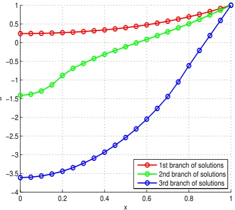
increasing of α. Now, we turn to see some multiple profiles which have been gathered in Figures 6
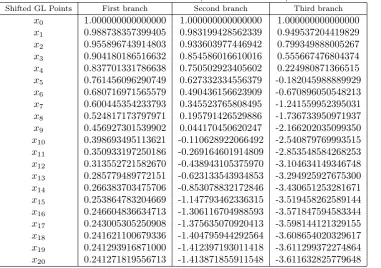
and 7 for those specified values of α and β in subsection 2.2.2. Figure 6 indicates that the original
problem (1.3)–(1.4) admits dual solutions in the case α = 0.5 and β = −0.2,−0.1. Also, Figure 7
0 0.2 0.4 0.6 0.8 1 0
0.1 0.2 0.3 0.4 0.5 0.6 0.7 0.8 0.9 1
x
u(x)
alfa=0 alfa=0.2 alfa=0.4 alfa=0.6 alfa=0.8 alfa=1 alfa=1.2 alfa=1.4 alfa=1.6 alfa=1.8 alfa=2
Figure 4: Dimensionless reactant concentration profiles with β= 1.
0 0.2 0.4 0.6 0.8 1
0.7 0.75 0.8 0.85 0.9 0.95 1
x
u(x)
beta=1 beta=2 beta=3 beta=4 beta=5 beta=6 beta=7 beta=8 beta=9 beta=10
Figure 5: Dimensionless reactant concentration profiles with α= 1.
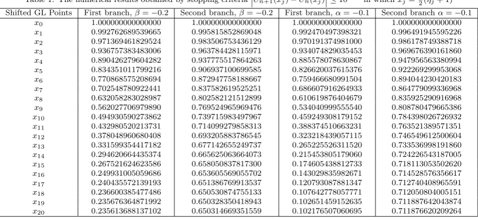
Table 1: The numerical results obtained by stopping criteria
Un+1(xj)−Un(xj) ≤10
−10in whichx
j= 12(ηj+ 1)
Shifted GL Points First branch,β=−0.2 Second branch,β=−0.2 First branch,α=−0.1 Second branchα=−0.1
x0 1.000000000000000 1.000000000000000 1.000000000000000 1.000000000000000
x1 0.992762689539665 0.995815852869048 0.992470497398321 0.996491945595226
x2 0.971369461829524 0.983506753436129 0.970191374981000 0.986178749388718
x3 0.936757383483006 0.963784428115971 0.934074829035453 0.969676390161860
x4 0.890426279604282 0.937775517864263 0.885578078630867 0.947956563380994
x5 0.834351011799216 0.906937100699585 0.826620037615376 0.922269299953068
x6 0.770868575208694 0.872947758188667 0.759466680991504 0.894044230420183
x7 0.702548780922441 0.837582619525251 0.686607916264933 0.864779099336968
x8 0.632058283028987 0.802582121512899 0.610619876404679 0.835925290916968
x9 0.562027706979890 0.769524965969476 0.534040999555540 0.808780479665386
x10 0.494930590273862 0.739715983497967 0.459249308179152 0.784398026726932
x11 0.432980520213731 0.714099279858313 0.388374510663231 0.763521389571351
x12 0.378048960680408 0.693205883786545 0.323218439057115 0.746549612500604
x13 0.331599354417182 0.677142655249737 0.265225526311520 0.733536998191860
x14 0.294620664435374 0.665625063664073 0.215453805179060 0.724226543187005
x15 0.267521624623586 0.658050837817300 0.174605438812733 0.718113053502620
x16 0.249931005059686 0.653605569055702 0.143029835982671 0.714528576356617
x17 0.240435572139193 0.651386769913537 0.120793087881347 0.712740408965591
x18 0.236600385477486 0.650530874755133 0.107642778057771 0.712050804005151
x19 0.235676364871992 0.650328350418943 0.102651459152635 0.711887642043874
0 0.2 0.4 0.6 0.8 1 0
0.1 0.2 0.3 0.4 0.5 0.6 0.7 0.8 0.9 1
x
u
1st branch of solutions for beta=−0.2
2nd branch of solutions for beta=−0.2 1st branch of solutions for beta=−0.1
2nd branch of solutions for beta=−0.1
Figure 6: Dimensionless dual reactant concentration profiles whenα= 0.5.
0 0.2 0.4 0.6 0.8 1 −4
−3.5 −3 −2.5 −2 −1.5 −1 −0.5 0 0.5 1
x
u
1st branch of solutions 2nd branch of solutions 3rd branch of solutions
Figure 7: Dimensionless triple reactant concentration profiles when α= 6 and β= 1.
4. Conclusions
Table 2: The numerical results obtained by stopping criteria
Un+1(xj)−Un(xj)
≤10
−10in which x
j =12(ηj+ 1)
Shifted GL Points First branch Second branch Third branch
x0 1.000000000000000 1.000000000000000 1.000000000000000
x1 0.988738357399405 0.983199428562339 0.949537204419829
x2 0.955896743914803 0.933603977446942 0.799349888005267
x3 0.904180186516632 0.854586016610016 0.555667476804374
x4 0.837701331786638 0.750502923405602 0.224980871366515
x5 0.761456096290749 0.627332334556379 -0.182045988889929
x6 0.680716971565579 0.490436156623909 -0.670896050548213
x7 0.600445354233793 0.345523765808495 -1.241559952395031
x8 0.524817173797971 0.195791426529886 -1.736733950971937
x9 0.456927301539902 0.044170450620247 -2.166202035099350
x10 0.398693495113621 -0.110628922066492 -2.540879769993515
x11 0.350933197250186 -0.269164601914809 -2.853548584268253
x12 0.313552721582670 -0.438943105375970 -3.104634149346748
x13 0.285779489772151 -0.623133543934853 -3.294925927675300
x14 0.266383703475706 -0.853078832172846 -3.430651253281671
x15 0.253864783204669 -1.147793462336315 -3.519458262589144
x16 0.246604836634713 -1.306116704988593 -3.571847594583344
x17 0.243005305250908 -1.375635070920413 -3.598144121329155
x18 0.241621100679336 -1.404795944292564 -3.608654020329617
x19 0.241293916871000 -1.412397193011418 -3.611299372274864
x20 0.241271819556713 -1.413871855911548 -3.611632825779648
References
[1] S. Abbasbandy, Approximate solution for the nonlinear model of diffusion and reaction in porous catalysts by means of the homotopy analysis method, Chem. Eng. J. 136 (2008) 144–150.
[2] S. Abbasbandy, E. Magyari and E. Shivanian, The homotopy analysis method for multiple solutions of nonlinear boundary value problems, Commun. Nonlinear Sci. Numer. Simulat. 14 (2009) 3530–3536.
[3] S. Abbasbandy and E. Shivanian, Prediction of multiplicity of solutions of nonlinear boundary value problems: Novel application of homotopy analysis method, Commun. Nonlinear Sci. Numer. Simulat. 15 (2010) 3830–3846. [4] S. Abbasbandy and E. Shivanian,Exact analytical solution of a nonlinear equation arising in heat transfer, Phys.
Lett. A 374 (2010) 567–574.
[5] S. Abbasbandy and E. Shivanian, Predictor homotopy analysis method and its application to some nonlinear
problems, Commun. Nonlinear Sci. Numer. Simulat. 16 (2011) 2456–2468.
[6] S. Abbasbandy and E. Shivanian, Multiple solutions of mixed convection in a porous medium on semi–infinite interval using pseudo–spectral collocation method, Commun. Nonlinear Sci. Numer. Simulat. 16 (2011) 2745–2752. [7] R. Aris,The Mathematical Theory of Diffusion and Reaction in Permeable Catalysts: The theory of steady state,
Vol. 1, Clarendon Press, 1975.
[8] E. Babolian, M. Bromilow, R. England and M. Saravi, A modification of pseudo–spectral method for solving a linear odes with singularity, Appl. Math. Comput. 188 (2007) 1260–1266.
[9] R.L. Burden and J.D. Faires,Numerical Analysis (third edition), Prindle, Weber and Smith, Boston, 1985. [10] C. Canuto, M. Hussaini, A. Quarteroni and T. Zang, Spectral methods in fluid dynamics, Springer Science &
Business Media, 2012.
[11] T. Clement, Y. Sun, B. Hooker and J. Peterson,Modeling multispecies reactive transport in ground water, Ground Water Monit. Remediat. 18 (1998) 79–92.
[12] E. Elbarbary and M. El–Kady,Chebyshev finite difference approximation for the boundary value problems, Appl. Math. Comput. 139 (2003) 513–523.
[13] A. Ellery and M. Simpson,An analytical method to solve a general class of nonlinear reactive transport models, Chem. Eng. J. 169 (2011) 313–318.
[14] B.A. Finlayson,The Method of Weighted Residuals and Variational Principles, Vol. 73. SIAM, 2013.
[15] E.J. Henley and E.M. Rosen,Material and Energy Balance Computations, John Wiley & Sons, New York, 1969.
[16] M.A.K. Ibrahim and R.S. Temsah, Spectral methods for some singularly perturbed problems with initial and
[17] C.T. Kelley,Iterative methods for linear and nonlinear equations, Front. Appl. Math. 16 (1995) 575–601. [18] A.H. Khater and R.S. Temsah,Numerical solutions of some nonlinear evolution equations by Chebyshev spectral
collocation methods, Int. J. Comput. Math. 84 (2007) 305–316.
[19] J.M. Ortega and W.C. Rheinboldt,Iterative solution of nonlinear equations in several variables, Vol. 30, SIAM, 1970.
[20] T.J. Rivlin,Chebyshev Polynomials, John Wiley & Sons, New York, 1990.
[21] Y. Sun, S. Liu and K. Scott, Approximate solution for the nonlinear model of diffusion and reaction in porous catalysts by the decomposition method, Chem. Eng. J. 102 (2004) 1–10.
[22] E.W. Thiele,Relation between catalytic activity and size of particle, Ind. Eng. Chem. 31 (1939) 916–920. [23] L.N. Trefethen,Spectral methods in MATLAB, Vol. 10, SIAM, 2000.